Abstract
High-definition maps (HDM) for autonomous driving (AD) are an important component of AD systems. HDMs accurately provide a priori information, including lane lines, and road signs, for AD systems. It is an important task to make a reasonable accuracy assessment of the HDM. The current methods for relative accuracy evaluation of general maps in the field of mapping are not fully applicable to HDMs. In this study, a method based on point set alignment and resampling is used to evaluate the relative accuracy of lane lines, and experiments are conducted based on relevant real HDM data. The results show that the relative accuracy of the lane lines is more detailed and relevant than the traditional method. This has implications for the quality control of HDM production.
1. Introduction
Autonomous driving (AD) technology relies on artificial intelligence, visual measurement, radar technology, and global positioning systems that operate in tandem to achieve safe autonomous vehicle operation. In the technical implementation of AD, high-definition maps (HDMs) are one of the fundamental parts. The main service object of the AD HDMs is the AD system, which collects data and then generates a specific map of a driving environment and builds environment and road models according to the needs of an AD system. It also provides a large amount of accurate and semantically rich data to help an AD system understand the surrounding environment at a finer scale, thus ensuring an over-the-horizon perception capability, which represents a basis for vehicle decision control and realization of intelligent driving. This denotes a basis for vehicle decision-making and control, and meets the needs of many high-level applications in the intelligent era [1,2].
AD technology can be roughly classified into six levels, according to the system operating conditions and roles assigned to the system in the driving task. Different levels of AD have different demands for HDMs. The classification of HDMs according to the Society of Automotive Engineers (SAE) AD levels and the corresponding requirements for each level are given in Table 1. There are a total of 6 (0 to 5) levels of AD that utilize different maps from traditional, statics, dynamic, and smart HDMs.

Table 1.
Classification of AD Levels and Their Demands for Maps.
Generally, it has been believed that there is no immediate need for HDMs for AD below Level 3, and that Advanced Driving Assistance System (ADAS) data and traditional navigation map data can meet the demand for maps and related data for Level 3 AD. From Level 3 of AD onward, the subject of environment perception transfers from a driver to the AD system, and HDMs for AD are necessary in this case [3,4]. As Level 3 of AD relates only to a specific environment and requires constant driver intervention, the requirements for autonomous driving HDMs are relatively low, and map data do not need to be dynamically updated in real-time. Levels 4 and 5 of AD denote complete AD in a specific or random environment [5], and do not require driver intervention, so the requirements for AD HDMs are higher and maps are required to be updated in real-time according to relevant traffic events. Therefore, the maps become dynamic, intelligent, HDMs.
Compared to general electronic navigation maps, autonomous driving HDMs are characterized by a large amount of data, rich elemental information, and higher accuracy requirements. There have been many studies on data acquisition methods of autonomous driving HDMs, including data acquisition along specific routes by acquisition vehicles equipped with Global Navigation Satellite System (GNSS) Real-time Kinematic (GNSS-RTK) [6], through high-cost solutions, such as using LIDAR combined with vision sensors to extract road information, which is equipped with high-precision GNSS-RTK and inertial navigation systems that constitute a mobile road measurement system for acquisition [7]; and low-cost solutions, such as extracting road information by deep learning-based methods using HD remote sensing images and aerial photographs [8]. However, in these methods, there can be many errors in generated HDMs, which generally include GNSS combined inertial guidance positioning errors, multi-sensor time synchronization and calibration errors, in-vehicle laser and camera sensor measurement errors, and machine recognition road information extraction errors.
Ordinary navigation maps have an accuracy from 5 m to 10 m [1,9], and can depict only the location, shape, and attributes of a road without providing more detailed information, such as location, shape, and attributes of lane lines, various road signs, and junction indicators. HDMs are used in AD systems, which require information on exact vehicle position in a lane and attributes of different lanes to achieve accurate control of a vehicle; thus, more details and a higher accuracy are required than in ordinary navigation maps. The AD industry generally defines that absolute and relative accuracies of a HDM for AD should be within 1 m and 20 cm, respectively [2,10,11]. Owing to multiple error sources and the required high accuracy of HDMs, a reliable, accurate, and stable evaluation of map accuracy is necessary. By relying only on feature point pairs that can be easily found both on the map and in the actual measurement, the traditional method is not relevant for the evaluation of some parts where these point pairs are difficult to find. This limitation leads to the fact that traditional methods are not good at evaluating the fine details of HDMs.
At present, there is no systematic theory and method for accuracy evaluation of HDMs for AD, and traditional map accuracy evaluation methods are generally used for verification. However, HDMs serve AD systems, which are sophisticated automated systems, and the operation of the system is related to the safety of the occupants in AVs. In addition, the current HDM data are generally obtained from high-precision measurements, and the map data need to be updated frequently. However, for such a large amount of data, it is not economical to use high-precision measurement equipment frequently, so many studies on map updating based on crowdsourced data have emerged [12]. In this case, a suitable method is also needed to verify the accuracy of the HDM geometry data obtained from crowdsourced collection to ensure quality data. Therefore, a new method is needed to evaluate the accuracy of HDMs to make a more relevant and accurate commonly used map evaluation. This study addresses the inapplicability of traditional map accuracy assessment methods for the description of HDM details, and designs a method based on point resampling and alignment to validate its relative accuracy based on HDM data from a road environment in China. The aim is to evaluate the relative accuracy description of HDM details with a proposed method and compare it with the traditional one.
This study is organized as follows: Section 2 introduces the background related to the accuracy of HDMs for AD and describes the non-adaptability of existing methods when verifying HDMs. Section 3 introduces the data used in this study and the specific evaluation methods, in which 3.2 divides the method into two directions: lane heading and side direction. In Section 4, experiments are conducted with the proposed method and a comparison is made with the traditional method. The final chapter discusses the progress and limitations of this study and the future directions of progress.
2. High-Definition Maps and Accuracy
2.1. Accuracy and Precision in Mapping
In the surveying and mapping field, accuracy refers to the density or dispersion of the error distribution and indicates how close the individual observations are to the mathematical expectation.
The mathematical expectation of an observation represents a true value of the observation when it contains only chance errors but not systematic errors or coarse deviations. Accuracy is generally measured by a medium error, which represents the standard deviation in mathematical statistics. For certain observations, the medium error cannot reflect measurement accuracy; for instance, the accuracy of a unit length in length measurement is measured using a relative error, which is generally expressed as a ratio of the medium error to the observed value, known as a relative medium error. Corresponding to the relative error, the medium error is called the absolute error [13].
The accuracy index of topographic maps in China is divided into the accuracy of plane position and elevation accuracy, and the concepts of medium error and limit error are mainly used to measure how discrete or dense the error distribution is and measure the maximum value of error that can occur in the map, respectively [14,15]. In this study, the absolute and relative accuracy of maps are defined.
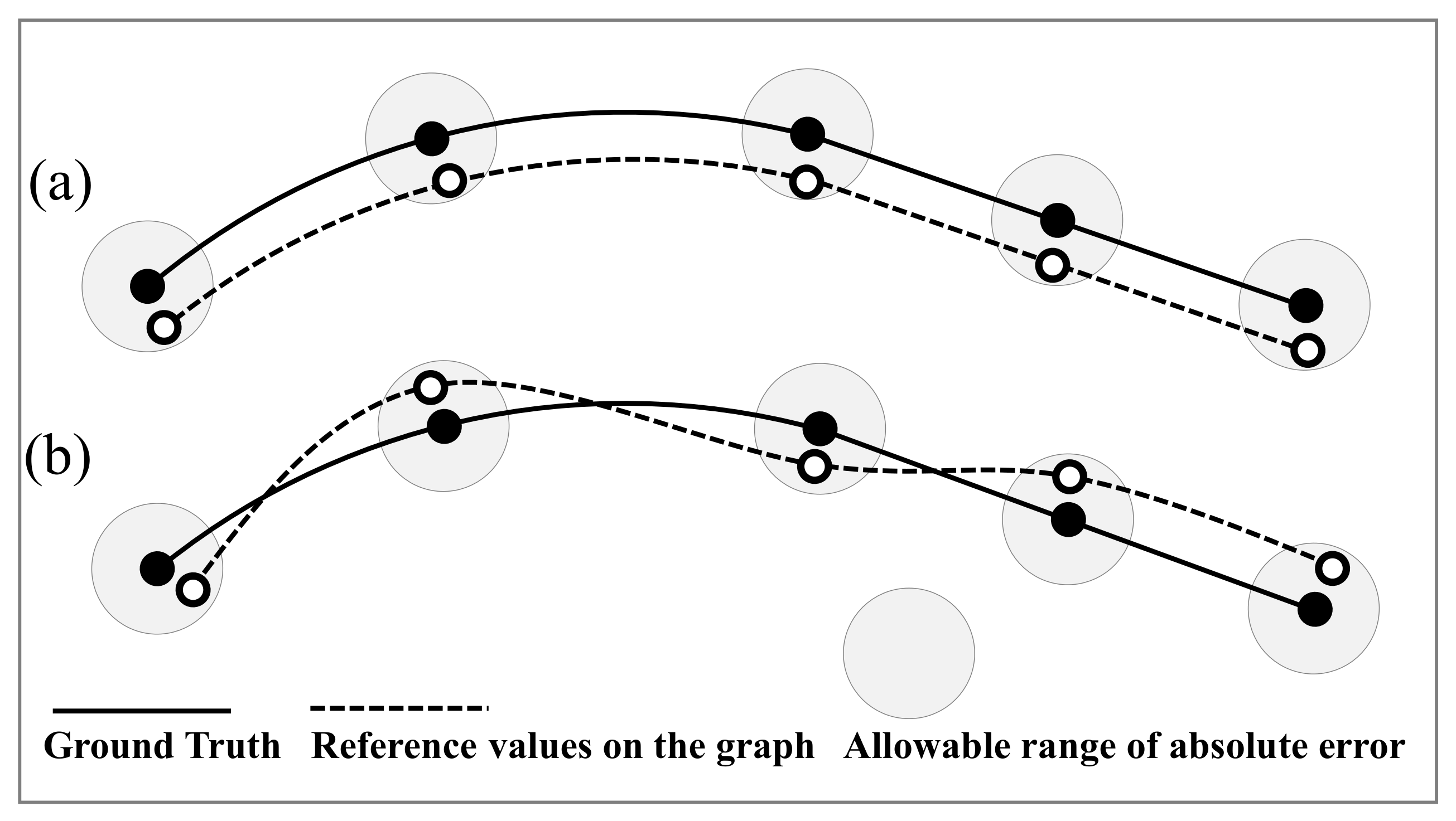
For maps, absolute accuracy denotes point accuracy, which represents an offset distribution of map points relative to their ground-truth points, whereas relative accuracy can be considered as a measure of deformation and retention of geometric shapes. The illustration of absolute and relative accuracy of a geometric shape is presented in Figure 1, where the solid line denotes the actual position of a lane line containing a curve with several feature points, whereas the dashed line shows the data curve to be verified containing the corresponding data feature points. As shown in Figure 1a, although the absolute error of the point position of each data feature is large and the overall accuracy is low, the overall geometry is well-maintained, and the relative error between the data feature points is small. Further, as shown in Figure 1b, although the absolute error of each data feature point is smaller than that in Figure 1a, the overall geometry of the curve is still distorted. This indicates that even when the absolute accuracy requirement of feature point locations is met, it is still possible for the overall data geometry to have a large distortion from the true geometry. In addition, there is another layer of meaning to the relative accuracy of HDMs, which is mainly reflected in the curve curvature smoothness. Compared to Figure 1b, the curvature of the data curve in Figure 1a is much smoother, making it more useful for the operation of autonomous vehicles.
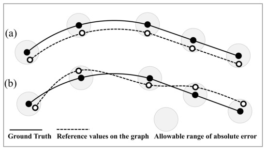
Figure 1.
Illustration of absolute and relative precisions of a geometric shape: (a) description of what is contained in the first panel; (b) description of what is contained in the second panel.
2.2. Accuracy in HDMs for AD
Although there are no strict standards for autonomous driving HDMs, the industry generally assumes that the absolute and relative accuracies of autonomous driving HDMs should be within 1 m and 20 cm, respectively. According to the demand-oriented analysis of autonomous driving HDMs, the absolute accuracy denotes the limit absolute error of feature points, whereas the relative accuracy denotes the limit relative error of feature points; generally, the limit error is two times the medium error. When verifying the accuracy of a HDM, a measurement result represents a feature point value relative to the true estimation value, so in the surveying and mapping field, the absolute accuracy of a HDM is the maximum value of the point error of a feature point relative to the corresponding true point value, which is generally regarded as the point limit error; whereas the relative accuracy is the maximum value of the ratio between deviation values of a distance between two feature points using the true spacing and the true length. The relative accuracy represents the relative limit error of a line segment between two characteristic points, which can be measured by normalizing the relative error to a value of 100 m of the true length. Low absolute accuracy indicates that the absolute error between the measured point and the true point, i.e., the limit error is large, while low relative accuracy means that the geometry of the map is deformed.
2.3. Traditional Method for Accuracy
In the traditional relative accuracy verification method, it is necessary to manually find the corresponding points in the HDM corresponding to the actual feature points in the elements to be verified and form the corresponding point pairs between them.
However, in the actual verification, since many lane lines are a smooth curve, as shown in Figure 1, it is difficult to find the feature point pairs in the middle of the curve as described above. In such a case, the method usually used is to create a connection with other elemental features, such as the start and endpoints of the lane line as feature points, and the lane line is generally used as the start point at the location where the lane line is created at a certain intersection, and the stop line of a vehicle intersecting the lane line at a certain intersection as the endpoint. The lane lines in the above data, the starting point and the endpoint, are determined in this way. Then, by this traditional method, the relative accuracy of this lane line is determined by a total of four points at the beginning and end of the two lines.
For the traditional relative accuracy evaluation method [16], the first step is to obtain the observed value and the true value of n feature points, which is the coordinate value for the map, and the true value is the high-precision measurement value for the accuracy evaluation. Thus, for n feature points, there are point pair combinations and the true values of the plane coordinates of each point on the two coordinate axes are and , and the measured values are and . The absolute error of each point in the direction of the two axes is calculated as , . Then, the relative error of all points on the two axes is calculated as , , where . So, the medium error of all points on the two coordinate axes is:
From this, the overall medium error is calculated by the formula:
and this value is the judgment index of the relative accuracy of plane coordinates. The relative accuracy of the elevation, as opposed to the relative accuracy of the plane, is:
2.4. Limitations of Traditional Methods
Although the existing relative accuracy assessment methods are well defined from the theoretical point of view, and are commonly used for topographic maps, they have certain limitations for HDMs and can cause problems in actual accuracy verification.
2.4.1. Finding the Same Feature Point Pair
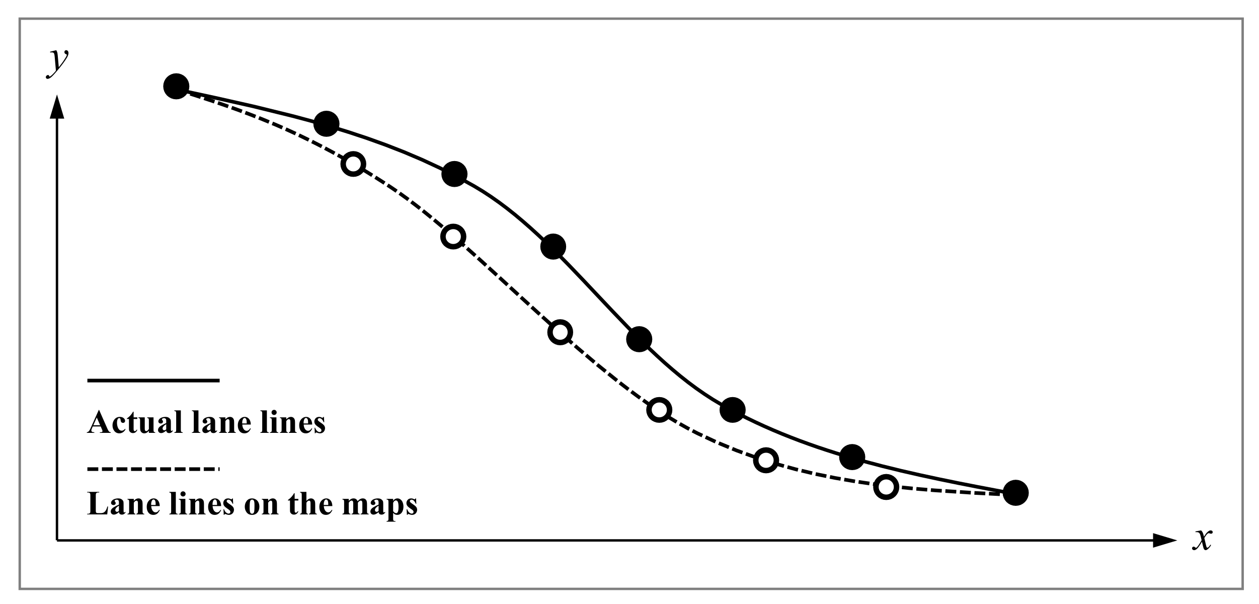
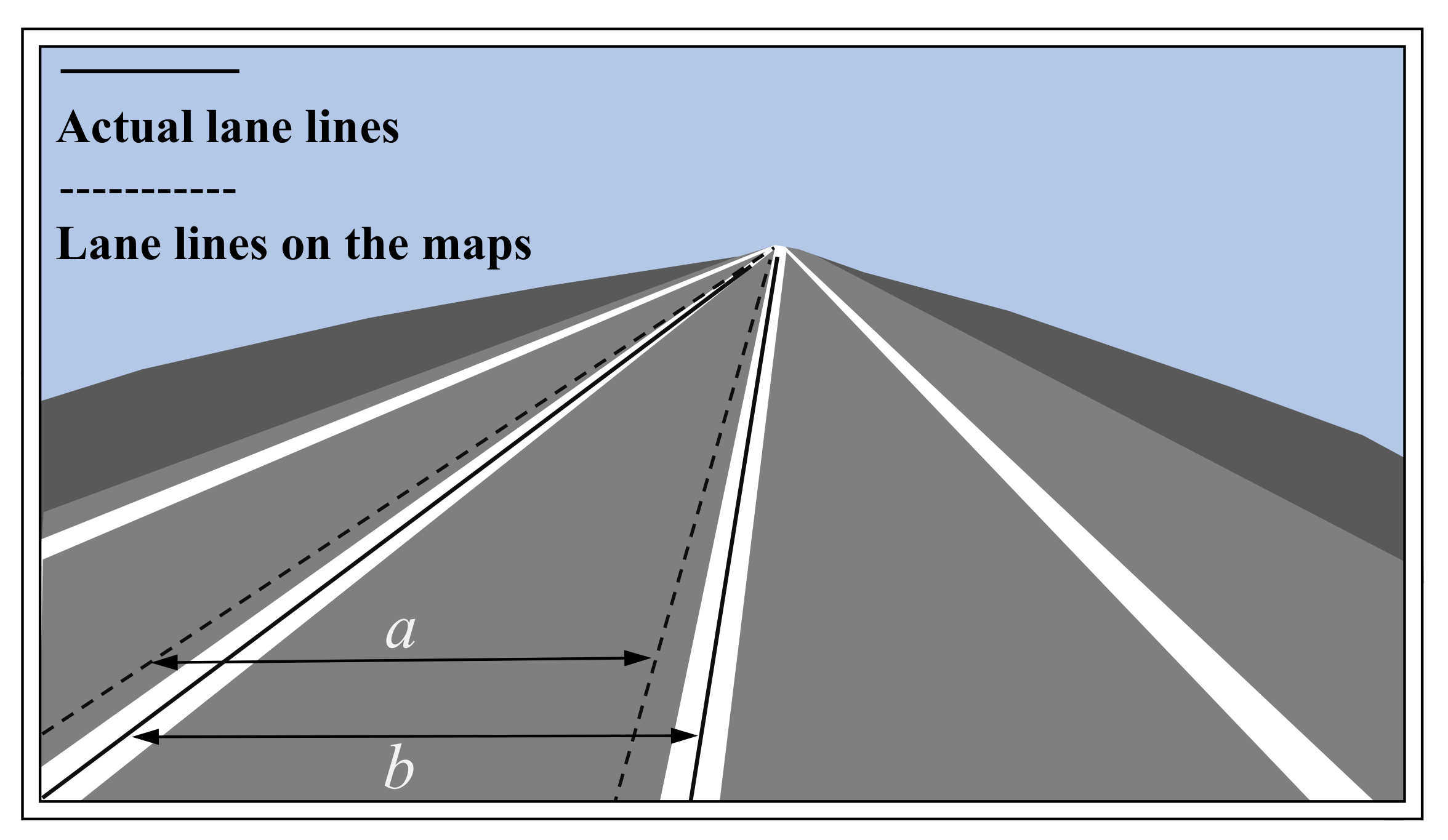
Autonomous driving HDMs provide rich and detailed information on their elements, but feature points can be difficult to find in detailed sections. For instance, in Figure 2, the start and end points of a lane line have small deviations from their true values, and it is difficult to find the homonymous point with the same name in the curve. Therefore, if the relative accuracy is evaluated by the calculation method of the relative accuracy definition introduced at the beginning of Section 2, which is based only on the ratio of distance deviations of start and end points to their true distance values, the relative accuracy will be high. For points on the curve with a large error, this method will be inaccurate.
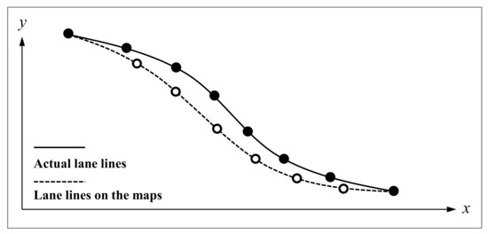
Figure 2.
Few feature points with the same name in the curved lane line.
2.4.2. Differences between Lane Heading and Side Directions
The lane lines are most representative in HDMs. From the point of view of usage demand of HDMs in AD, as shown in Figure 3, the significance of accuracy along the lane heading direction is different from that in the lane side direction. In the lane heading, self-driving vehicles need to combine HDM for their positioning, but a section of lane line in this direction is usually measured in hundreds of meters, the scale is large, and AD vehicle systems need their accurate position. In the lane bypass direction, the general lane width is approximately 3.75 m, and an AV only needs to determine which lane it is inside and in relation to; furthermore, the locating scale range is small [17].
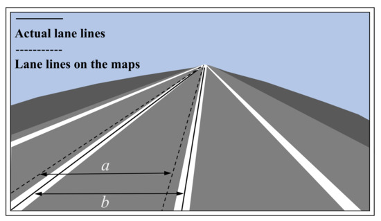
Figure 3.
Lane line sideways positioning accuracy requirements.
Considering the difference in the usage demand of HDMs in AVs in the lane heading and bypass directions, the above-mentioned assumption that the relative accuracy of HDMs for AVs should be within 20 cm should be differentiated in the heading and bypass verification.
2.5. Elemental Classification and Decomposition of HDMs
Since relative accuracy relates to deformation and retention of geometry, relative accuracy verification should be performed between at least two features. To make the verification of various geometric elements easier, geometric elements are decomposed.
The road model and data format of AD HDMs are significantly different from those of general electronic navigation maps. Therefore, to clarify the target objects of the accuracy evaluation of autonomous driving HDMs and to distinguish the accuracy evaluation methods of different object elements, elements contained in autonomous driving HDMs are decomposed.
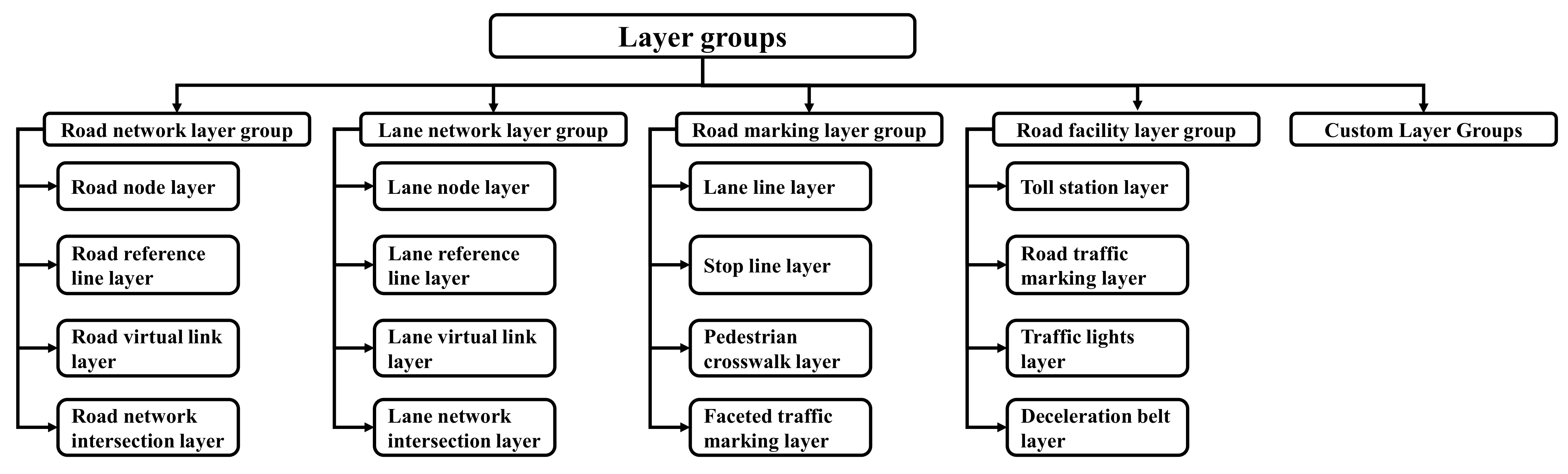
The AD HDMs can be roughly divided into several groups, including road networks, lane networks, road markings, and road facilities. The classification of maps in different groups is shown in Figure 4 [18].
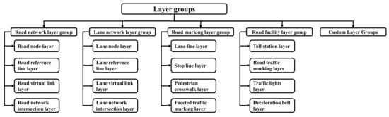
Figure 4.
Layer-based classification of autopilot HDMs.
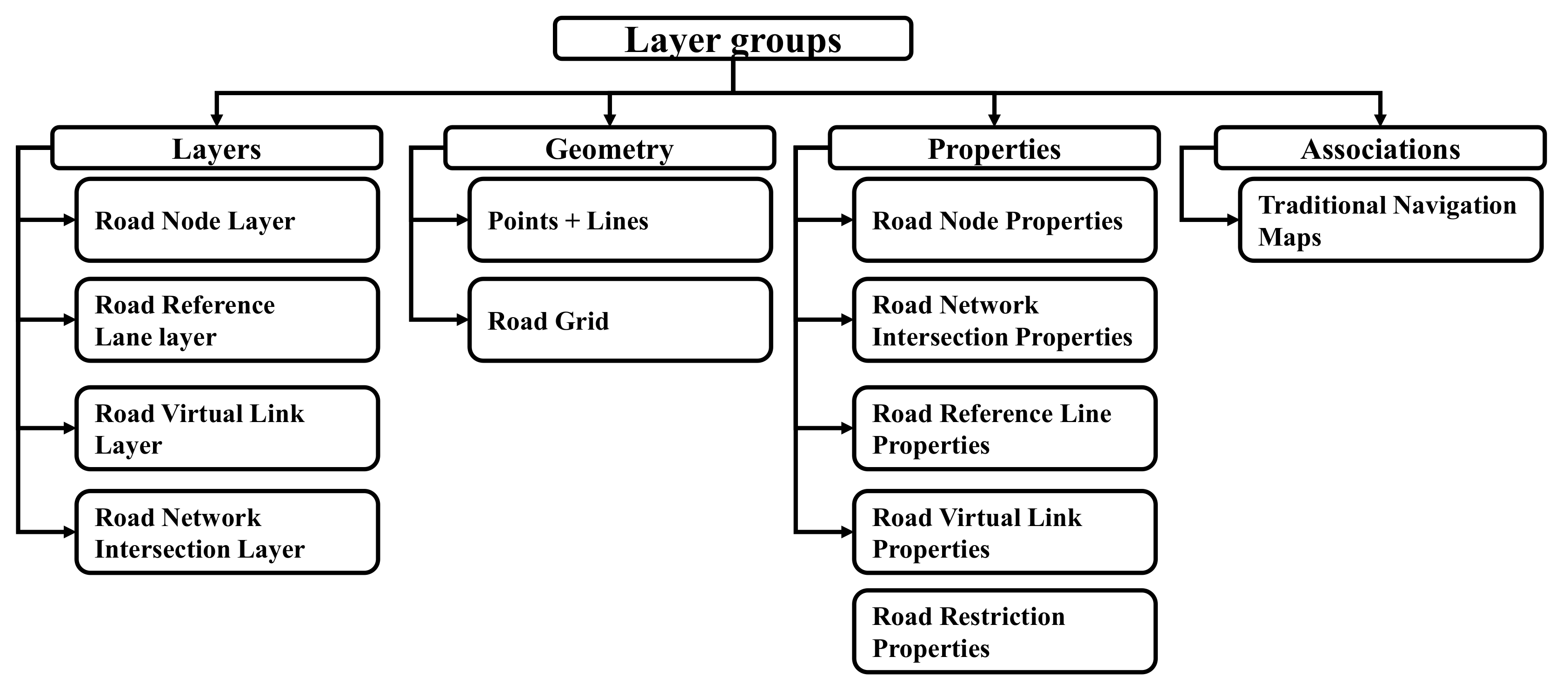
The data model of each group in Figure 4 is relatively similar. The data model of the road network layer group is shown in Figure 5. As this paper discusses only relative accuracy assessment of autonomous driving HDMs, only geometric data elements and other accuracy-related characteristics of each layer group of an autonomous driving HDM are introduced. The general requirements for autonomous driving HDMs, information on various attributes, association with other data, and map rendering are not introduced and discussed.
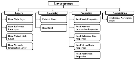
Figure 5.
The data model of the road network layer group.
The elements that should be included in a HDM for AD can be roughly categorized into the point, line, surface, and body elements according to their geometry and storage form. Specifically, point elements include road nodes, road network junctions, lane nodes, lane network junctions, lane line feature points, fire hydrants, and road sensing facilities. Line elements include road reference lines, road virtual connection lines, lane reference lines, lane virtual connection lines, stop lines, road projection, road markings, contour markings, line separation facilities, line crossing facilities, and poles. Surface elements include pedestrian crossings, surface traffic markings, road traffic signs, traffic lights, speed bumps, toll booths, checkpoints, surface cross-road facilities, car parks, on-street parking spaces, safety islands, and pole-less bus shelters. Body elements include general bus stops.
In the relative accuracy evaluation of point elements, the line connecting two feature points is transferred into a straight-line element for evaluation; each surface element is decomposed into several line elements that are evaluated. All types of geometric elements in an HDM are decomposed into two feature point connecting lines or line elements, on the basis of which the relative accuracy is evaluated.
Owing to differences in accuracy meaning and accuracy demand in the lane-heading and side directions of an HDM, the relative accuracy verification is divided into the lane-heading direction verification and lane-side direction verification. In the verification, the feature points and points on the curve of an HDM are measured by the high-precision method, and the high-precision measurement result is used as a true coordinate value of a point, while the point coordinate value in the existing map is used as a reference data value.
3. Materials and Methods
3.1. Case Study
The specific coordinates of the data used in this study and the location of the park cannot be disclosed in this study because some relevant policies and laws in China require that the real geographic information coordinates be confidential. Therefore, the presentation involving the experimental park will omit the coordinate information as well as the name, etc. All presentations about point measurements will also hide their coordinate information.
3.1.1. Equipment and Environment
The high-precision measurement equipment used for data acquisition was a GNSS receiver, using the Find CM service. This is a high accuracy positioning service product with a single measurement accuracy of centimeter-level, which is developed by network-based dual-frequency RTK technology and can provide an all-weather location service for most of the areas in China.
The experimental environment is an actual AD experimental demonstration site for which a Chinese third-party mapping company produced an AD HDM with the same organization and element classification rules as those described in Section 2. The overall area of the park is about 3.8 km2 and the total road mileage is about 22.4 km. It contains various general roads, parking lots, intersections, road appurtenances, etc. The width of each lane is between 3.5 m and 3.75 m. The road markings are clear and contain obvious curves and straight lines. However, the park is a general urban environment with no significant changes in overall elevation and no overly complex marking and road environment. In addition, thanks to the absence of tall buildings blocking the park, point measurements using GNSS technology are not greatly affected.
3.1.2. Data Acquisition
The lane line can actually be seen as a geometric surface of equal width (as it has a certain width to be observed by the driver), ranging from 10 to 15 cm wide. In the production of HDM for AD, the center line of the geometric surface is actually used as the lane line. Therefore, when conducting the evaluation, the midline of the marked lanes is also collected in the field.
When data collection is performed for each lane segment, the starting and ending points of this segment need to be determined. The starting point and endpoint are usually the points where the lane line appears at an intersection and ends at another intersection where the lane line disappears at the vehicle stop line.
In the actual measurement, the instrument is required to briefly measure at the point for 3 to 5 s to obtain multiple measurements for real-time measurement adjustment. This keeps the accuracy of this final measurement at the point within 1 cm, and satisfies the high accuracy measurements required for accuracy assessment. In addition to measuring the start and endpoints of a section of lane line, points on the midline of each section of lane line were also measured. To better reflect the specific details of the lane lines, measurements such as curved lane lines will be taken at small intervals of approximately one measurement per meter (and will be more intensive at locations of greater curvature).
The AD HDM data from a park were used to validate the proposed relative accuracy evaluation method. The experimental data included a set of lane lines containing complex curves. The lane lines were the center lines of the shape of the ground lane lines, and each set of lane lines contained the left and right lane lines of a certain lane.
3.2. Methodology
Comprehensively, as mentioned in Section 1, it is difficult to find the corresponding feature point pairs in the validation of the actual HDM, so this study adopts a point resampling-based alignment method. Specifically, the points on the curve to be verified are first fitted and sampled, then the point pairs are aligned, and then resampling is performed after the alignment is completed, and the relative accuracy calculation is completed on this basis.
After decades of development, there are various algorithms for aligning point pairs for different needs. The alignment algorithm used in this study is the iterative closet point (ICP) algorithm [19]. The advantage of this algorithm is the high accuracy of the matching calculation, and the disadvantage is the high requirement of the initial value and the large computational effort. In general, the ICP algorithm is appropriate for this study.
The basic flow of the ICP algorithm is as follows:
- Calculate the corresponding closet point in the target point set for each point in the source point set.
- Compute the rigid transformation that minimizes the average distance of the above corresponding point pairs. Calculate the rotation and translation parameters.
- The new point set is obtained by using the rotation and translation parameters found in 2, for the source point set.
- Determines if the iterative computation stop condition is met. If it is, the calculation is stopped, if not, the new point set obtained in 3 is used as the new source point set and input into 1 to continue the iterative calculation.
The common iteration stopping conditions are: the change in rotation and translation parameters is less than a certain threshold; the average distance between the set of transformed points and the set of target points is less than a certain threshold; the number of iterations reaches a certain threshold, etc.
The ICP algorithm for point set transformation results in the output of the transformed point set, along with the transformation parameters. The transformation parameters are usually expressed in the form of rotation and translation matrices. The rotation matrix can be decomposed into a matrix representation of the set of points rotated along each of the three axes of the right-angle coordinate system in space, as follows
The rotation angles along each of the three coordinate axes are . So, the overall rotation matrix is
The translation parameter is the value of the set of points to be translated along each of the three coordinate axes, and these values are then formed into a translation matrix in the order of the coordinate axes. After the transformation of the rotation and translation matrix, the point set can be transformed from the starting position pose in space to any position pose.
3.2.1. Lane-Heading Direction
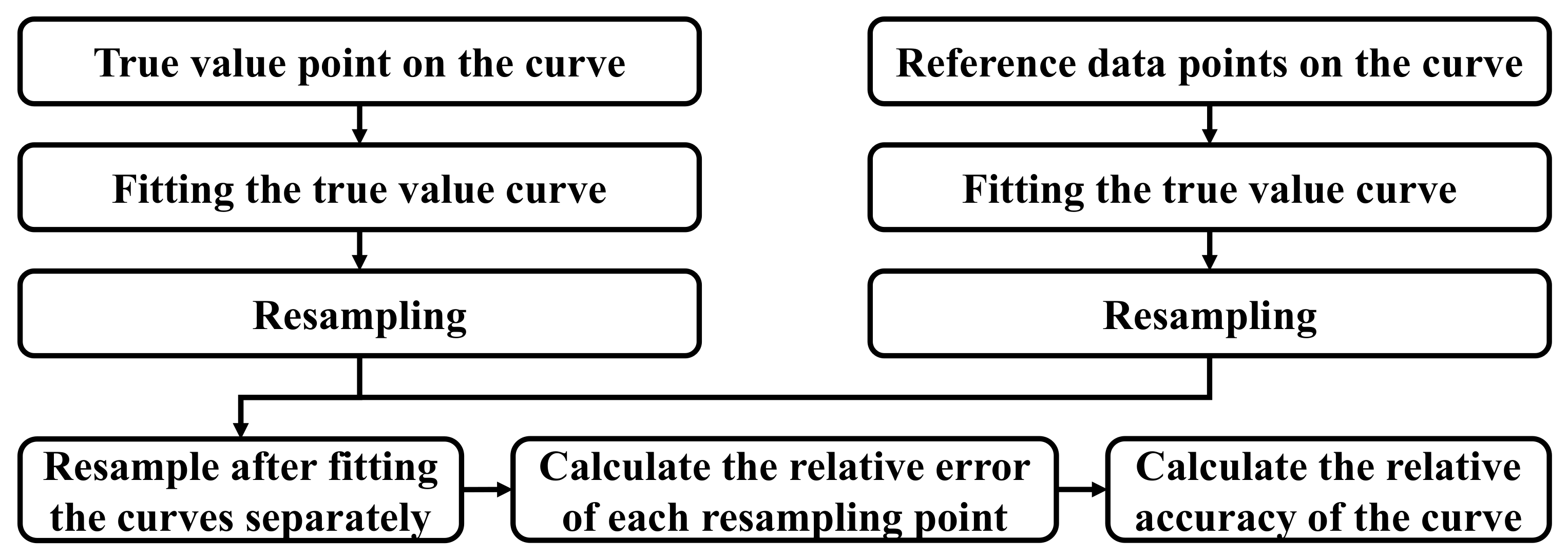
Considering that an actual lane line is variable and may contain various complex curves and straight-line elements, all line elements are evaluated as curves. The relative accuracy of line elements is evaluated using the flowchart presented in Figure 6.
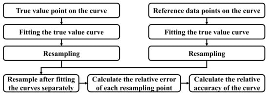
Figure 6.
Flowchart of the relative accuracy evaluation method of line elements.
The first step is to extract the ground truth points of elements of the curve to be evaluated and the data points on the graph, which do not have to correspond to each other. The curves passing through all the ground truth points and the data points on the graph are fitted separately and denoted as the truth curve and data curve, respectively. The true and data curves are sampled separately using a suitable sampling interval to obtain a number of sampling points. The true sample points are aligned with the data sample points by the iterative closest point (ICP) algorithm [19]. The intersection of the normal with the true curve represents the corresponding true coordinate point of a data point, and the distance between the two points represents the deviation of the data point. The ratio of all deviations relative to the true curve length is calculated and denoted as a relative error, and then the median error of all ratios is calculated. The median error is a relative error in the curve heading. For the whole map, after combining the median relative error of all validated elements, the median error is used as a limit error, i.e., the relative accuracy of the heading. In general, this relative accuracy can be converted to a value of 20 cm or less per 100 m of lane length.
3.2.2. Lane-Side Direction
This verification requires the involvement of the left and right lane lines of a section of a lane, i.e., the adjacent lane lines of a lane. The data points of the left and right lane lines on the graph are extracted separately and fitted to two data curves. The corresponding true coordinate values are then extracted and fitted to the two true curves. The true and data curves are sampled separately using a suitable sampling interval to obtain several sampling points. The true sampling points are aligned with the data sampling points by the ICP algorithm. Then, using one of the aligned data curves, e.g., the left data curve, as a reference, all data points on this data curve are calculated. The intersection of point a1 with the corresponding left true curve is called the corresponding true coordinate point b1, and the intersection of point a1 with the corresponding right data curve is called the corresponding data point a2. The normal of the left true curve is made over point b1, and the right true curve is intersected at point b2. The distance between points a1 and a2 is the data lane width m1 at data point a1, and the distance between points b1 and b2 is the corresponding real lane width n1 at point a1. The purpose of the ICP alignment is to find points on the real curve that correspond to data points and to calculate the data lane width at the corresponding point, as well as the real lane width. The absolute value of a difference between m1 and n1 is calculated and denoted as a relative error of the lane bypass at data point a1. The relative error is calculated for all data points to obtain the median lane bypass relative error, and then the limit error is obtained by multiplying the median error by two, which represents the lane bypass relative accuracy. This relative accuracy can be set to 20 cm.
After the data curve has been fitted to the real curve, the data points are normal to the data curve, and the intersection of the normal and real curves represents the corresponding point of each data point. The distances between data points and their corresponding points represent the deviations of data points. The median error of these deviations is calculated, and the limit deviation error, i.e., the relative accuracy of the lane bypass, is calculated as two times the median error.
After the alignment-based method is applied to the data, the midpoint of the curve and its corresponding points can be easily found, and deviation can be obtained to calculate the relative curve accuracy. This method avoids the distortion of a curve part during the calculation, making the evaluation process simpler and results more reliable.
4. Results
4.1. Results for Lane-Heading Direction
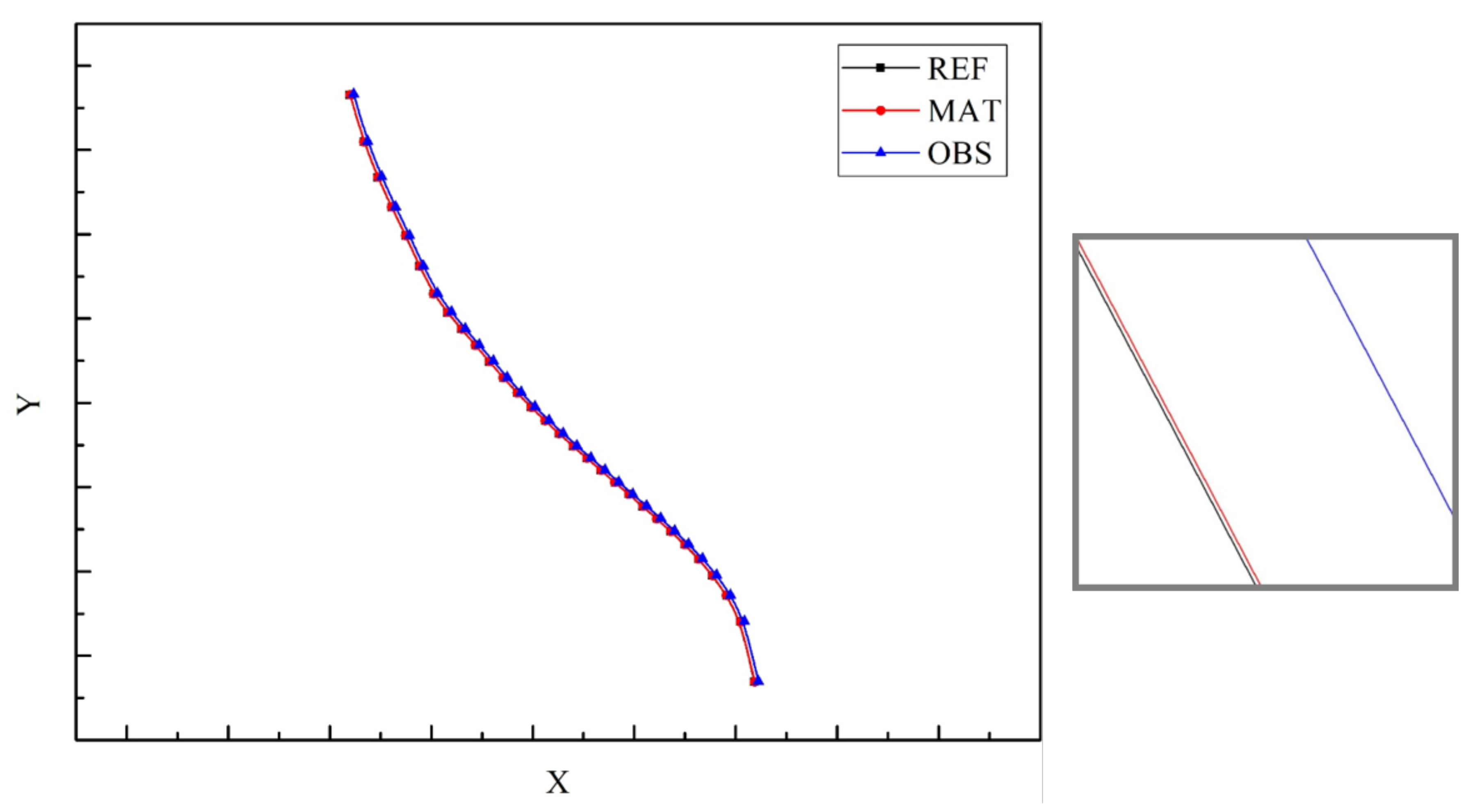
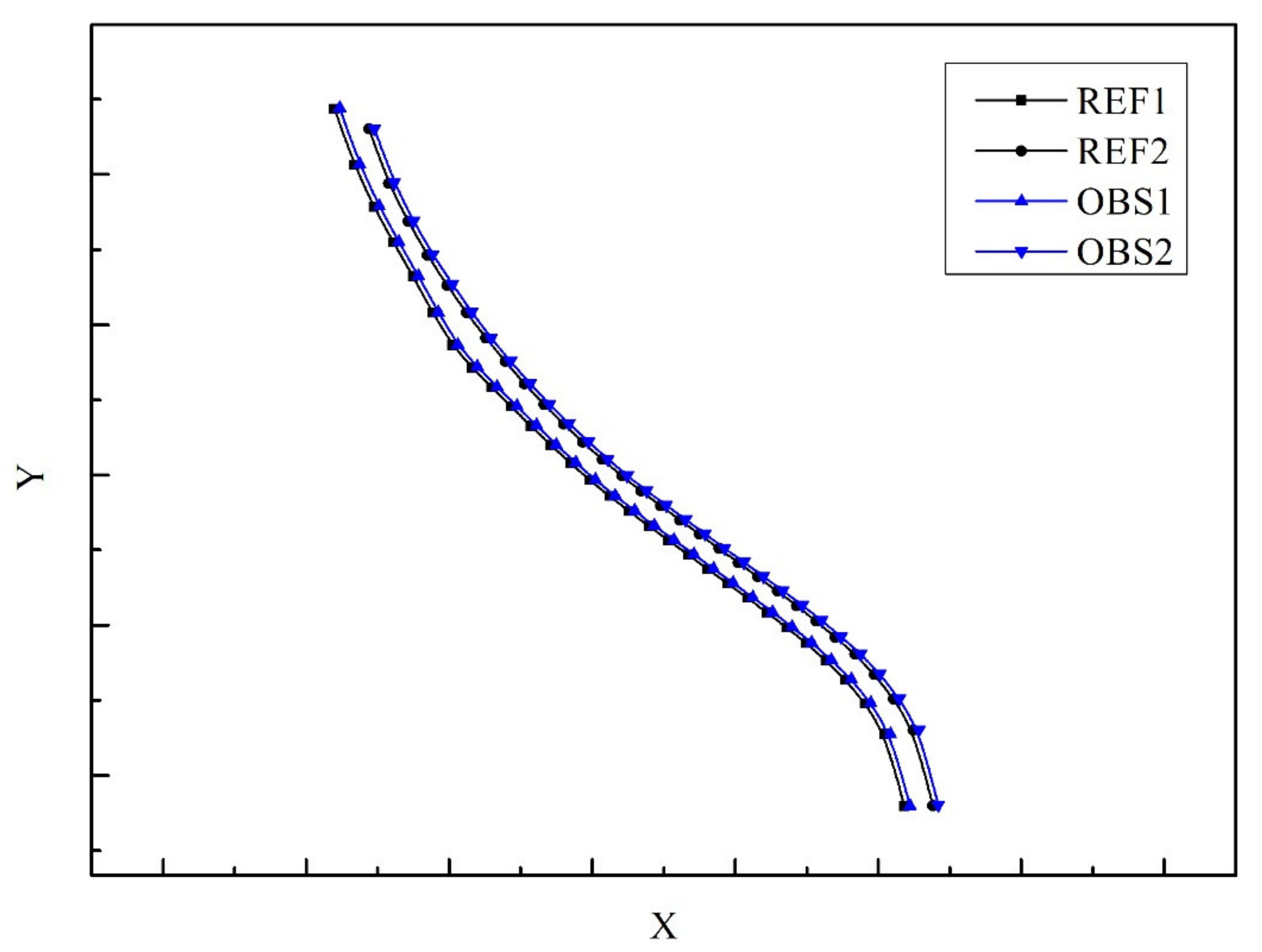
The true curve was fitted to the data curve and resampled, and the resampled points were aligned by the ICP algorithm. The alignment results are shown in Figure 7, where the figure on the right side represents a partial enlargement of the left figure.
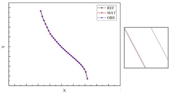
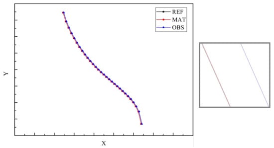
Figure 7.
One group of ICP-aligned lanes.
In Figure 7, the black curve represents the reference value (map data value) curve, the blue curve represents the observed value (verified true value) curve, and the red represents the post-match curve. To show the details of the above lines more clearly, the axes of the enlarged view are stretched. The first section of the lane line of rotation matrix R and translation matrix T of the ICP alignment are respectively expressed as
After alignment, the median deviation error of data points on the calculated curve was 13.6; the real length of this curve section was 166.8 m, so the median error of the calculated relative error was 0.082%, which attributed an error of 0.082 m to the 100 m lane line length yield. Since the limit error was two times the median error, the limit error of this section of the lane line was 0.164, which was less than 20 cm and thus could meet the relative precision requirement.
The other section of the lane line of rotation matrix R and translation matrix T of the ICP alignment are respectively expressed as
After alignment, the median deviation error of data points on the calculated curve was 0.128; the real length of this curve section was 166.2 m, so the median error of the calculated relative error was 0.077%, which attributed an error of 0.077 m to the 100 m lane line length yield. Since the limit error was two times the median error, the limit error of this section of the lane line was 0.154, which was less than 20 cm and thus could meet the relative precision requirement.
For a section of the lane, the relative accuracy depends on the average of the relative accuracy of the two-lane lines it contains. Therefore, the relative accuracy of this lane segment is 0.080. The limiting error for this lane section is 0.159.
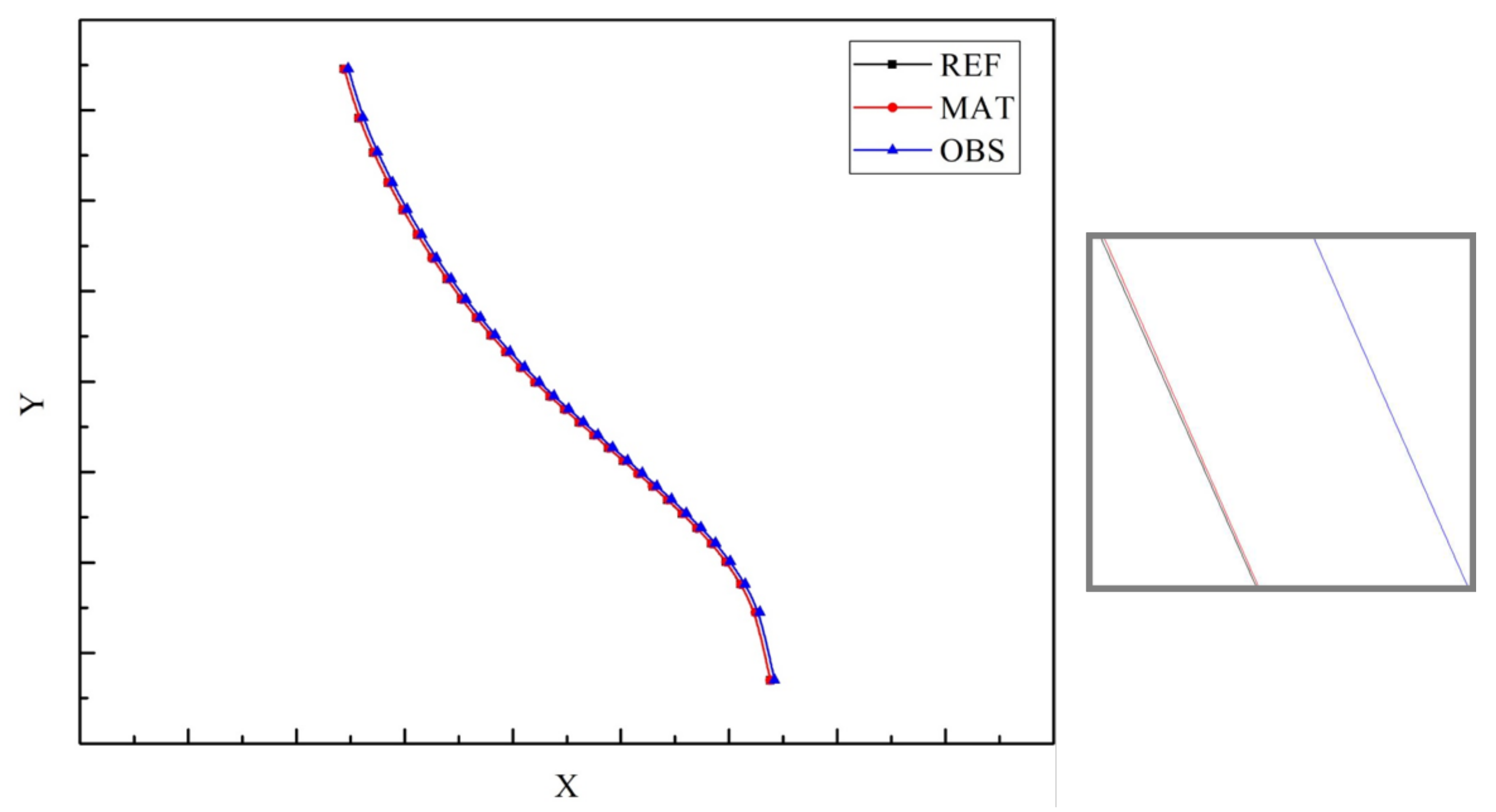
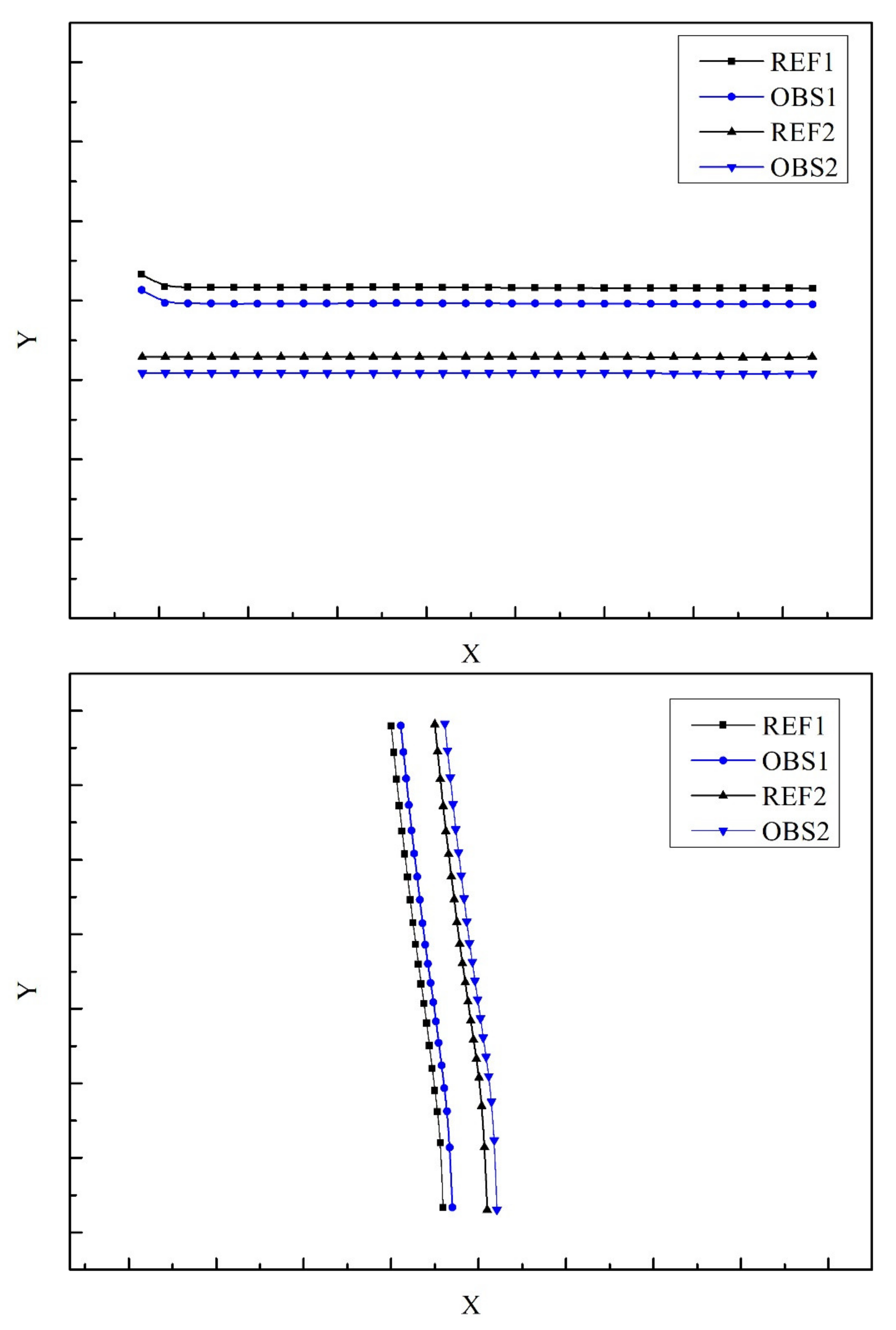
In addition to the section of lane shown above, there are three more sections of lane below in Figure 8, including a more typical straight lane with a more typical single curve. Similarly, the axes are stretched to show the details more easily.
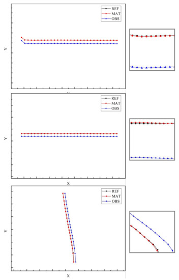
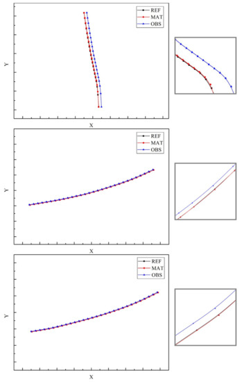
Figure 8.
Three additional groups of ICP-aligned lanes.
The results of the above four-lane groups aligned by this study are presented in Table 2.
Table 2.
Results of the relative accuracy of four sets of lane lines.
4.2. Results for Collinear Direction
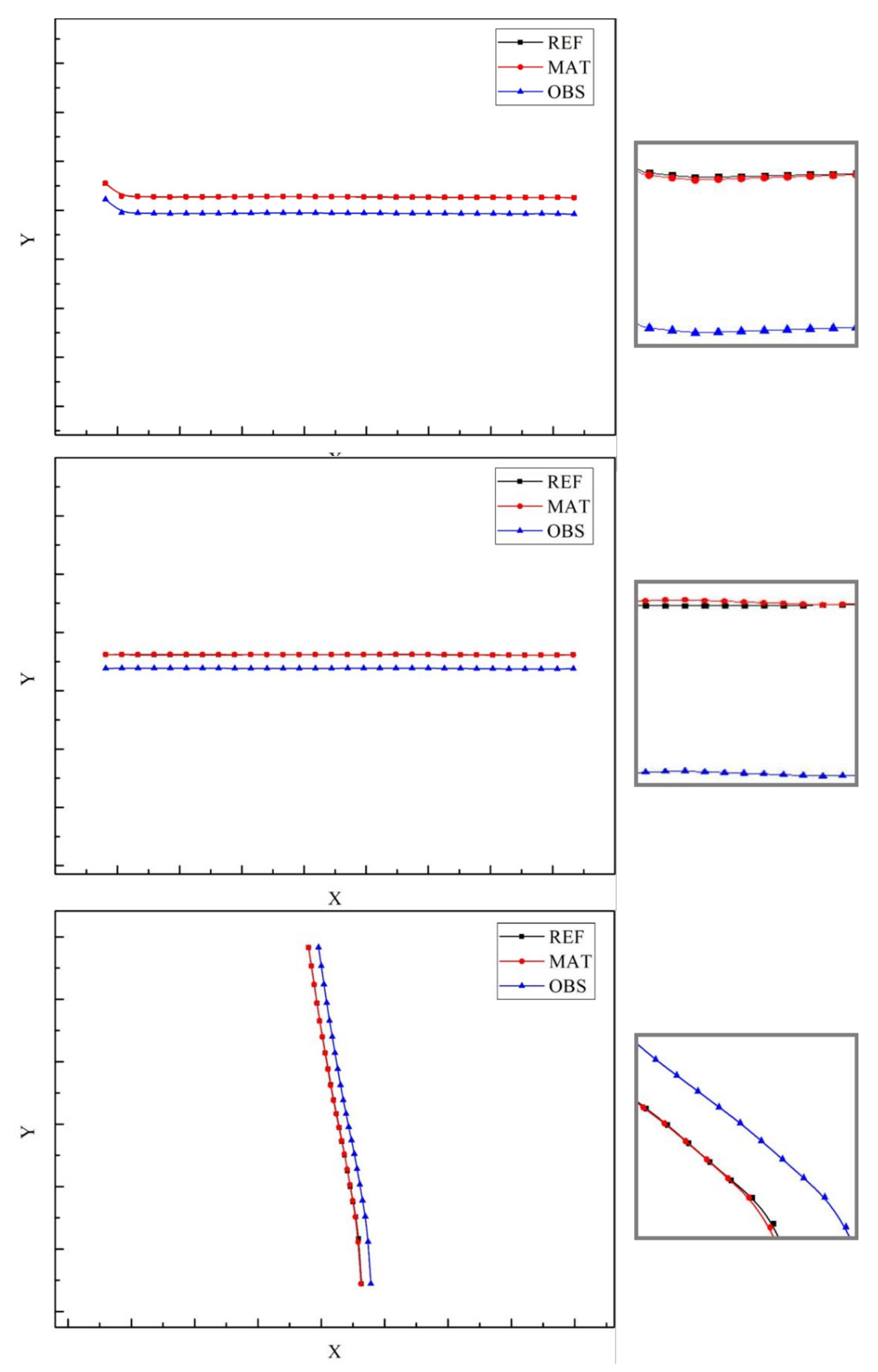
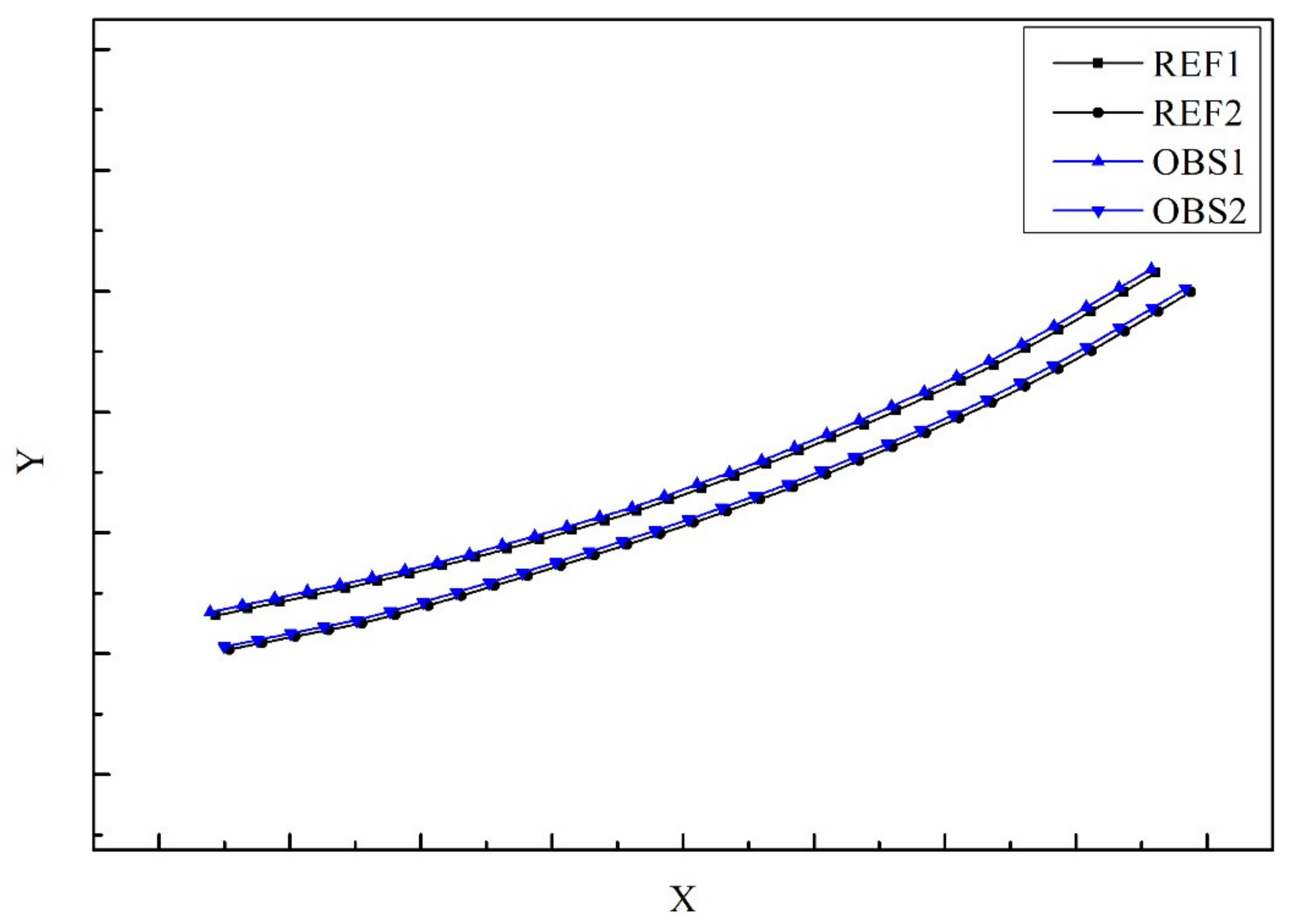
The true curve was fitted to the data curve and resampled. The resampled points were aligned by the ICP algorithm, and the alignment results are shown in Figure 9, the two diagrams show the left and right lane lines contained in a section of lanes, respectively.
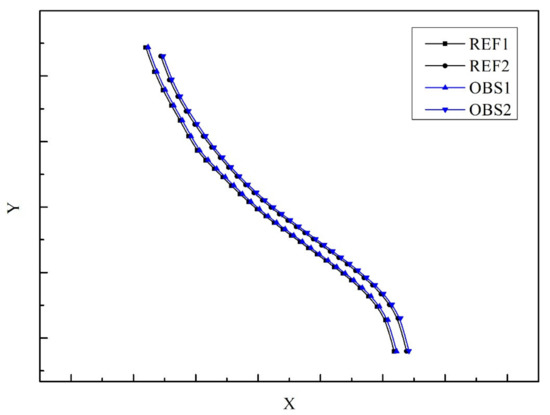
Figure 9.
Relative accuracy evaluation between adjacent lanes of the first lane.
In Figure 9, the black curve represents the reference value (map data value) curve, and the blue curve represents the observed value (verified true value) curve. The first section of the lane of rotation matrix R and the translation matrix T of the ICP alignment are respectively expressed as
After alignment, the median difference error between the true curve lane width and the data curve lane width was calculated to be 4.5 cm. Therefore, the limit error of the lane width deviation of this lane line, which was two times the median error, was 9 cm, which is less than 20 cm and thus could meet the relative precision requirement.
In addition to the section of lane shown above, there are three more sections of lane below in Figure 10, including a more typical straight lane with a more typical single curve.
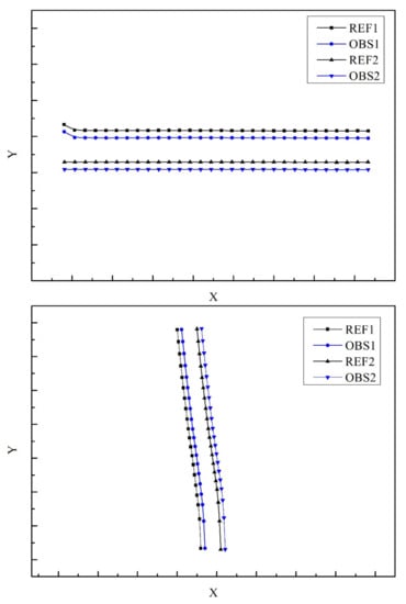
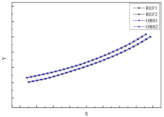
Figure 10.
Relative accuracy evaluation between adjacent lanes of the other three lanes.
The results of the above four-lane groups aligned by this study are presented in Table 3.
Table 3.
Results of the relative accuracy of four sets of lane lines.
4.3. Results of Traditional Methods
In summary, the relative accuracy index of the three-dimensional spatial point set was divided into plane relative accuracy index and elevation relative accuracy index. In each set of lanes used for the experiment, only four points are available (as they are the only ones that contain the corresponding observations and measurements). Then, n equals four. In this way, in the first group of lanes, according to the above formula, the relative accuracy of the vertical is calculated to be 0.091 and the relative accuracy of the horizontal is calculated to be 0.0025. The remaining groups of lanes calculated by the conventional method are shown in Table 4 below.
Table 4.
Results of the relative accuracy of four sets of lane lines.
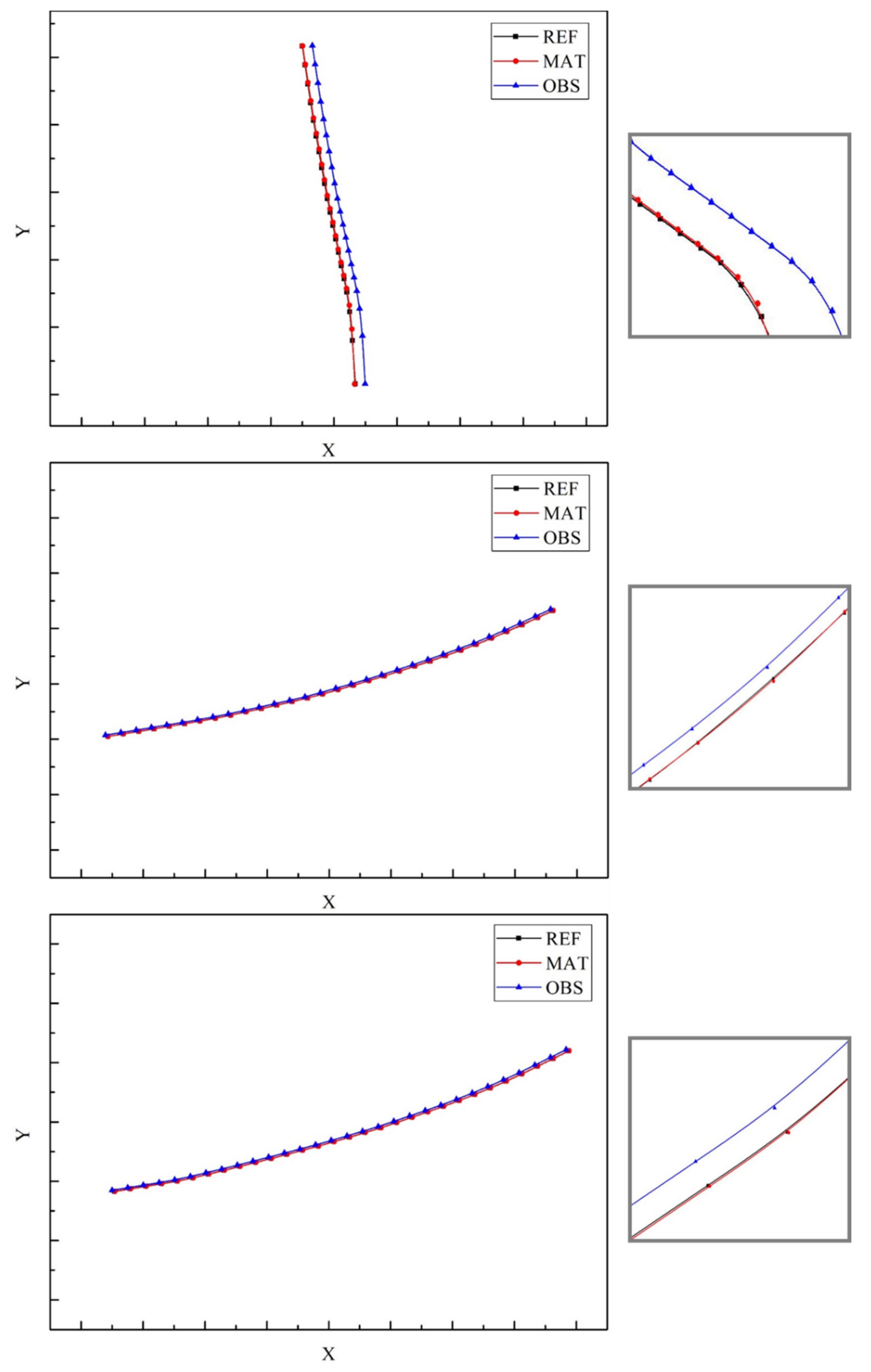
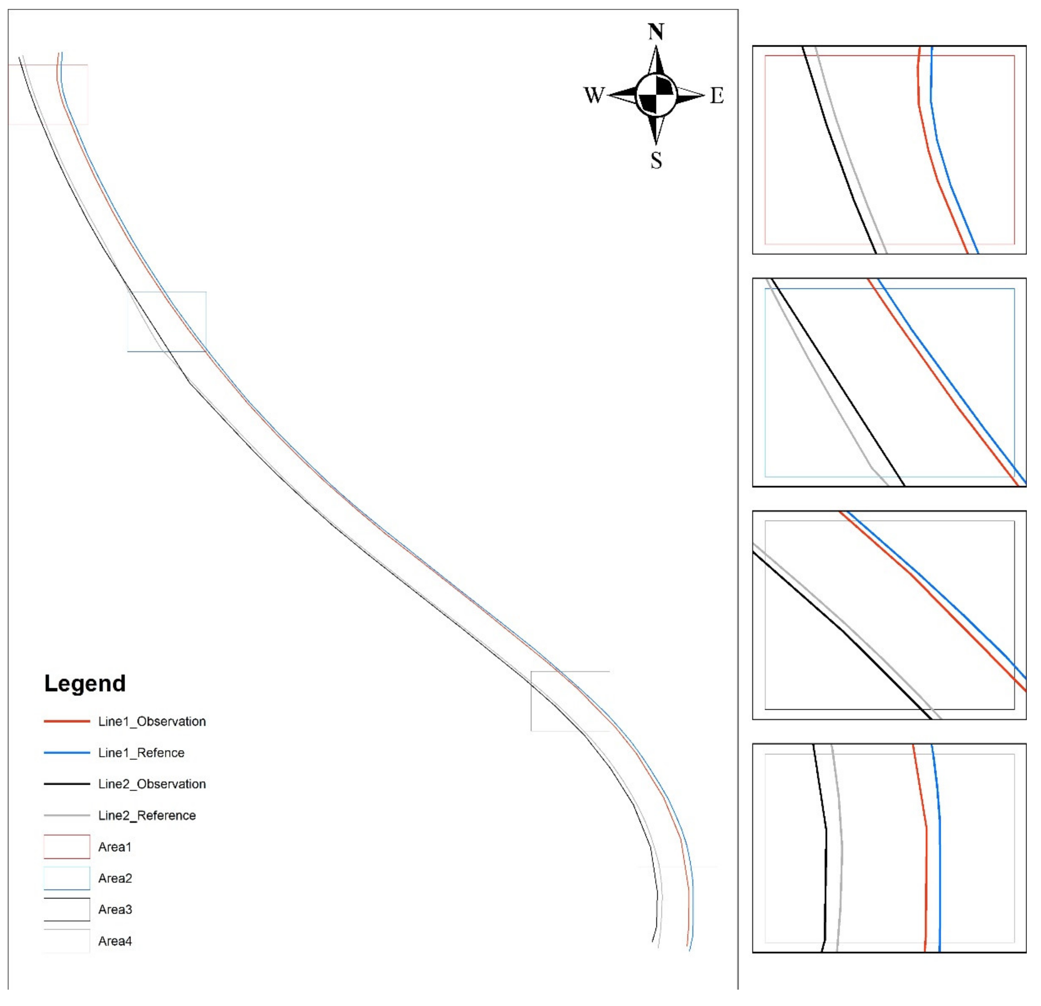
Using the results calculated for the first lane segment as an example, the small value of the medium error in the elevation direction obtained by the traditional method indicates that the relative accuracy of the measurement in the elevation direction of these data is high; the value of the medium error in the plane is also smaller than that obtained by the method in this paper, indicating that the traditional method considers the relative accuracy in the plane of this section of the lane to be high as well. However, the calculated data for the conventional method here only contain a total of four points at the start and end of each of the two lines. Therefore, the relative accuracy calculated by the traditional method is actually only for these four points, while the relative offset deformation between the above four points is small, so the relative accuracy calculated is higher. As a result, the traditional method does not provide a complete and relevant description of the entire lane line. This can be verified by looking at all points along the entire lane line.
As shown in Figure 11, there is a significant distortion of the curve on the map in the middle of the lane line relative to the end of the lane line, which is not well represented in the values calculated by the traditional method. In contrast, the method of this paper performs better in this case.
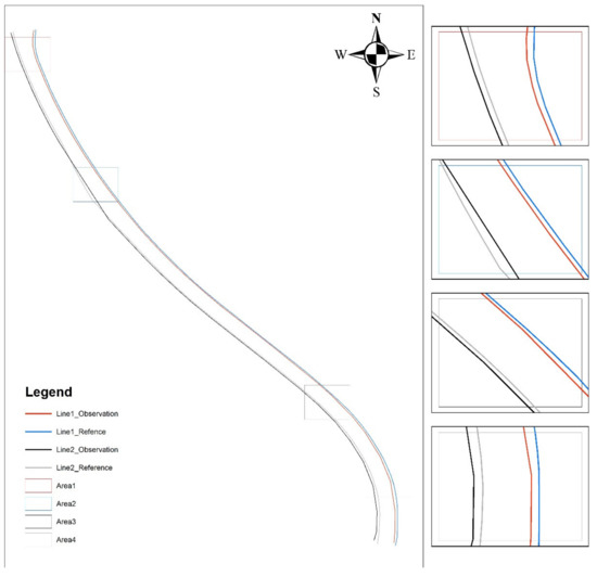
Figure 11.
The size of the deformation differs significantly between the curves.
Similar conclusions can be drawn with the results of the calculations for the remaining groups of lanes. The second group of lanes is a set of nearly straight lines, and in the results of this group of lanes, both the method of this paper and the traditional method give a better result, which is because the accuracy of the HDM is better at both ends and the middle of this straight section, so the results of both methods are similar. In the results of the last two-lane groups, different results are reflected again, for reasons similar to those of the first group of lanes, both because the traditional method only considers the coordinates of the four endpoints and does not make use of the data in the middle of the lane line.
5. Discussion
In this study, a method based on point resampling and alignment was used to evaluate the accuracy of some actual HDMs. The results show that in lane lines lacking curvature variation, the accuracy obtained by this paper’s method is similar to that of the traditional method, while in lane lines containing distinct curves, this method evaluates the fine details of the HDMs more finely and closely than the traditional method. A finer evaluation of the HDM means that we can better control the quality of the HDM, which is crucial for the localization and decision making in the driving of autonomous vehicles. Without an accurate and reliable map, it is impossible to operate the vehicle reliably.
We compared the method in this paper with the traditional method in our experiments, and the results are more different in the lane lines containing curves. The traditional method relies on feature point pairs, while in the case of curves, only the start and end points of the lane lines can be relied on. The shape of the middle of the curve is then not involved in the consideration. The method in this paper instead relies on point resampling and point set alignment to identify multiple corresponding point pairs in the curve, which will all be involved in the evaluation of this segment of the lane line. In this way, points exist at various locations along a lane line for evaluation. In addition to this, we also separate the evaluation of the lane line heading from the side direction, one dedicated to the evaluation of the deformation of a single lane line and the other dedicated to the evaluation of the relative deformation between two lines of a lane. This is more useful for how self-driving vehicles can determine their position in the lateral direction of the lane.
However, due to the limitations of the data currently available to the authors, this paper cannot make conclusions for more complex road conditions. This study uses a small amount of data and a relatively homogeneous road condition of only 22 km long town roads in the plain area. The type of roads is also relatively homogeneous, and the performance of the method in this study cannot be verified in complex situations, such as mountain roads, complex overpasses, culverts, etc. Secondly, the final relative accuracy calculation is not consistent with the traditional relative accuracy calculation, we can only determine that the details of the roadway are better reflected in this paper’s method, but we cannot determine whether the numbers calculated by this traditional method and this paper’s method have the same validity between them.
The next part of this study can be a more comprehensive judgment of the ability of this method to evaluate the accuracy of HDMs in terms of enriching the data situation and testing the validity between the figures of this method and the traditional method. This is necessary in order to make a more comprehensive and detailed accuracy evaluation of HDMs, control the data quality of HDMs, and ensure the operational safety of AD systems.
Author Contributions
Conceptualization, Tengfei Yu, He Huang; methodology, Tengfei Yu and He Huang; software, Tengfei Yu; validation, Tengfei Yu, He Huang and Nana Jiang; formal analysis, Tengfei Yu, Tri Dev Acharya; investigation, Tengfei Yu and Nana Jiang; resources, He Huang; data curation, Tengfei Yu and Nana Jiang; writing—original draft preparation, Tengfei Yu, Nana Jiang; writing—review and editing, He Huang, Tri Dev Acharya; visualization, Tengfei Yu, Tri Dev Acharya; supervision, He Huang, Tri Dev Acharya; project administration, He Huang; funding acquisition, He Huang. All authors have read and agreed to the published version of the manuscript.
Funding
This research received no external funding.
Institutional Review Board Statement
Not applicable.
Informed Consent Statement
Not applicable.
Data Availability Statement
The data presented in this study are available on request from the corresponding author. The data are not publicly available due to the data itself involves absolute geographical coordinates and is classified as state secret data. However, the data used in this paper are only examples and the reader can reproduce the methods in this paper in any dataset.
Conflicts of Interest
The authors declare no conflict of interest.
References
- Liu, J.; Zhan, J.; Guo, C.; Lei, T.; Li, Y. Data Logic Structure and Key Technologies on Intelligent High-precision Map. J. Geod. Geoinf. Sci. 2020, 3, 1–17. [Google Scholar]
- Liu, R.; Wang, J.; Zhang, B. High Definition Map for Automated Driving: Overview and Analysis. J. Navigation 2020, 73, 324–341. [Google Scholar] [CrossRef]
- Levinson, J.; Montemerlo, M.; Thrun, S. (Eds.) Map-Based Precision Vehicle Localization in Urban Environments. In Robotics: Science & Systems III, June; Georgia Institute of Technology: Atlanta, GA, USA, 2007. [Google Scholar]
- Chi, G.; Wenfei, G.; Guangyi, C.; Hongbo, D. A lane-level LBS system for vehicle network with high-precision BDS/GPS positioning. Comput. Intell. Neurosci. 2015, 2015, 7. [Google Scholar]
- Heiko, G.; Seif, H.X. The key challenge of the self-driving car industry in smart cities-high-definition maps. Engineering 2016, 2, 27–35. [Google Scholar]
- Sutarwala, B.Z.J.D.; Gradworks, T. GIS for Mapping of Lane-Level Data and Re-Creation in Real Time for Navigation. 2011. Available online: https://escholarship.org/content/qt56m28858/qt56m28858.pdf (accessed on 7 September 2021).
- Schreiber, M.; Knoppel, C.; Franke, U. (Eds.) LaneLoc: Lane marking based localization using highly accurate maps. In Proceedings of the Intelligent Vehicles Symposium (IV), Gold Coast, QLD, Australia, 23–26 June 2013. [Google Scholar]
- Hou, Q.; Li, B.; Cai, Y. High-precision lane-level map elements extracting based on high-resolution remote sensing image. Bull. Surv. Mapp. 2021, 3, 38–43. [Google Scholar]
- Cai, Y.; Zhang, W.; Yan, Q.; Wang, X.; Bai, J.; Ma, X. Position accuracy and its test method for navigation digital maps. J. Navig. Position. 2021, 9, 10–14. [Google Scholar]
- Levinson, J.; Thrun, S. (Eds.) Robust Vehicle Localization in Urban Environments Using Probabilistic Maps. In Proceedings of the IEEE International Conference on Robotics & Automation, Anchorage, AK, USA, 3–7 May 2010. [Google Scholar]
- Fairfield, N.; Urmson, C. (Eds.) Traffic light mapping and detection. In Proceedings of the IEEE International Conference on Robotics & Automation, Shanghai, China, 9–13 May 2011. [Google Scholar]
- Kim, K.; Cho, S.; Chung, W. Hd map update for autonomous driving with crowdsourced data. IEEE Robot. Autom. Lett. 2021, 99, 1895–1901. [Google Scholar] [CrossRef]
- Wuhan University School of Surveying and Mapping Survey Leveling Discipline Group. Error Theory and Fundation of Surveying Adjustment-Second Edition; Wuhan University Press: Wuhan, China, 2009; ISBN 978-9-307-06896-4. [Google Scholar]
- Specifications for Quality Inspection and Acceptance of Surveying and Mapping Products, GB/T 24356-2009. 2009. Available online: http://www.cssn.net.cn/cssn/productDetail/f9f6f180a88e0246cf80283a1b52ff48 (accessed on 30 September 2009).
- Basic Requirements for Products of Digital Topographic Map, GB/T 17278-2009. 2009. Available online: http://www.cssn.net.cn/cssn/productDetail/5b693051528fa9474332a95d083acd3c (accessed on 6 May 2009).
- ISO 19157: 2013 Geographic Information—Data Quality. ISO 14041:2013(E), International Standards Organization. Available online: https://www.iso.org/standard/32575.html (accessed on 7 September 2021).
- Reid, T.; Houts, S.E.; Cammarata, R.; Mills, G.; Agarwal, S.; Vora, A.; Pandey, G. Localization Requirements for Autonomous Vehicles. Preprint 2019, 2, 173–190. [Google Scholar] [CrossRef] [Green Version]
- Liu, J.; Wu, H.; Guo, C.; Zhang, H.; Zuo, W.; Yang, C. Progress and Consideration of High Precision Road Navigation Map. Strateg. Study CAE 2018, 20, 99–105. [Google Scholar] [CrossRef]
- Besl, P.J.; Mckay, N.D.; Intelligence, M. A method for registration of 3-D shapes. IEEE Trans. Pattern Anal. Mach. Intell. 1992, 14, 239–256. [Google Scholar] [CrossRef]
Publisher’s Note: MDPI stays neutral with regard to jurisdictional claims in published maps and institutional affiliations. |
© 2021 by the authors. Licensee MDPI, Basel, Switzerland. This article is an open access article distributed under the terms and conditions of the Creative Commons Attribution (CC BY) license (https://creativecommons.org/licenses/by/4.0/).