
Air Pollutant Concentration Prediction Based on a CEEMDAN-FE-BiLSTM Model


Abstract
:1. Introduction
2. Research Methods
2.1. CEEMDAN
2.2. FE
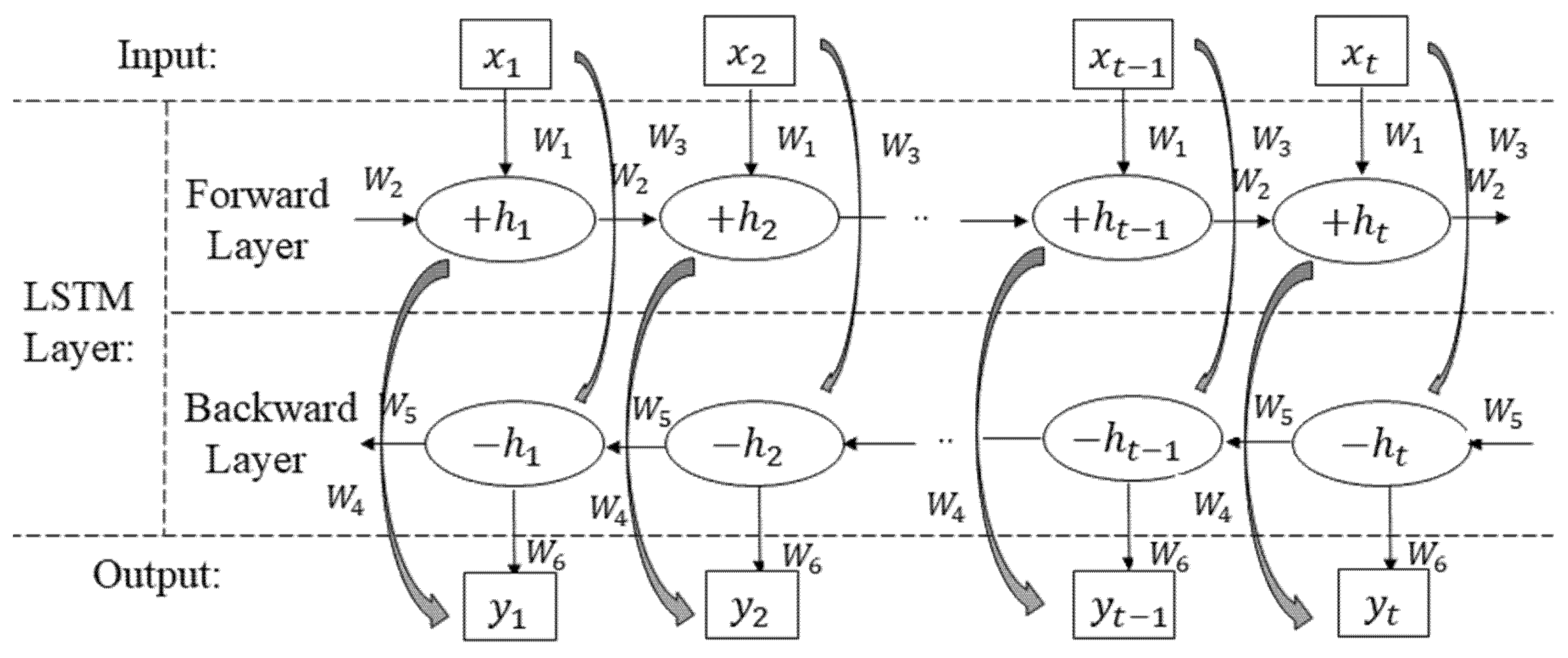
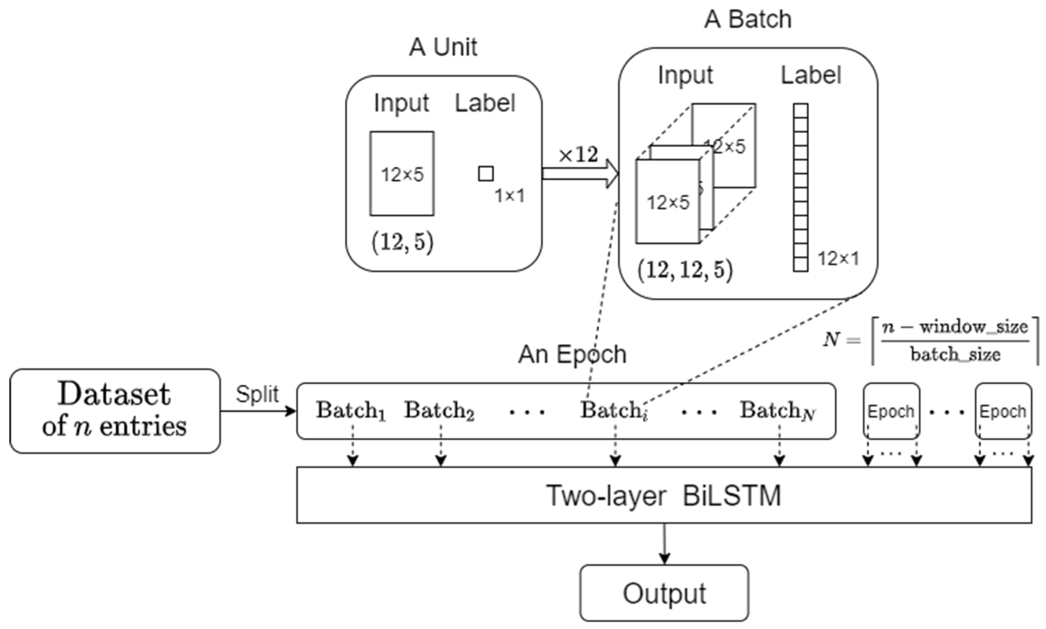
2.3. BiLSTM
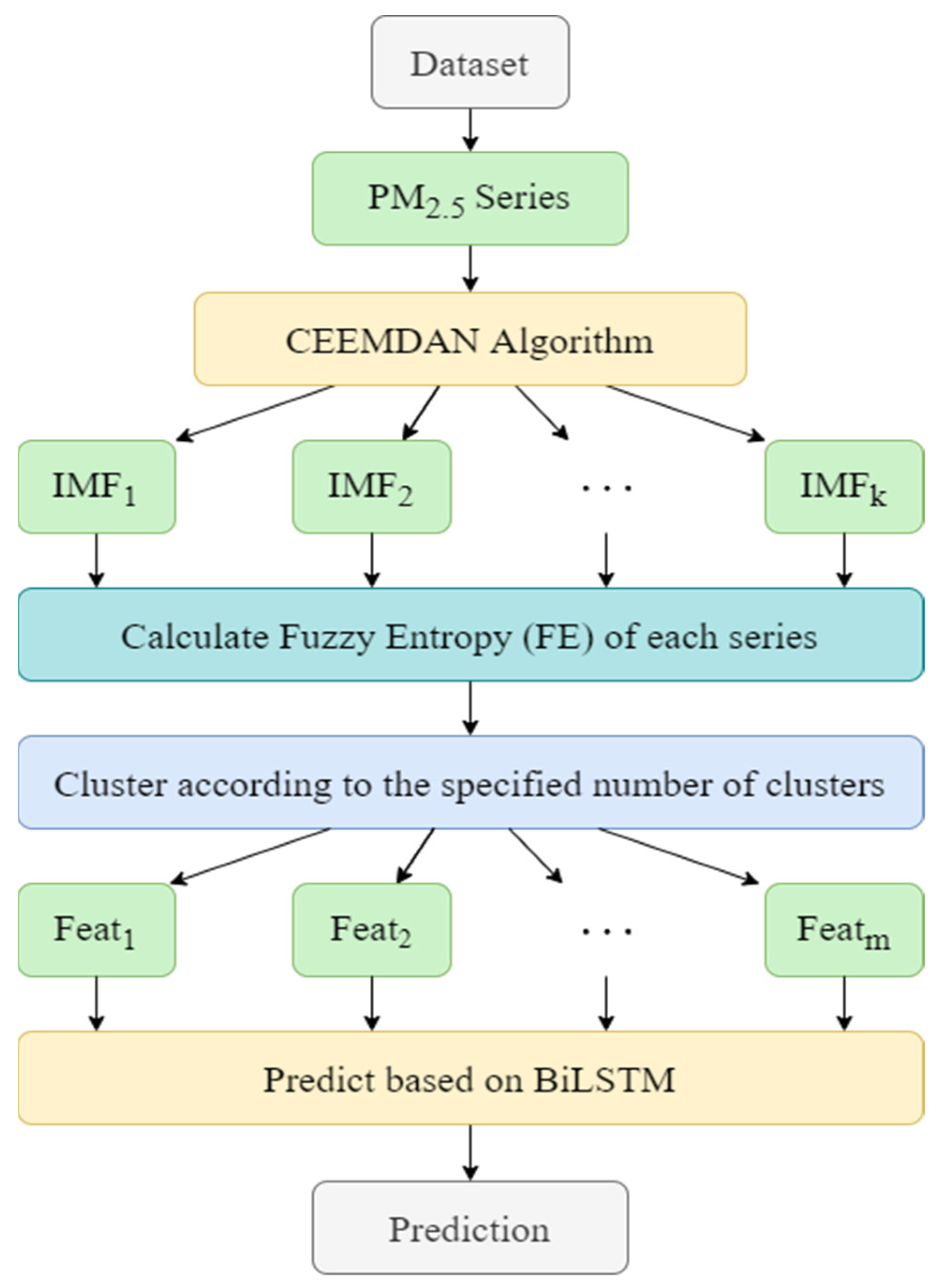
2.4. CEEMDAN-FE-BiLSTM
3. Experimental Analysis
3.1. Data Sources
3.2. Evaluation Criteria
3.3. Experimental Setup
3.4. Experimental Results and Analysis
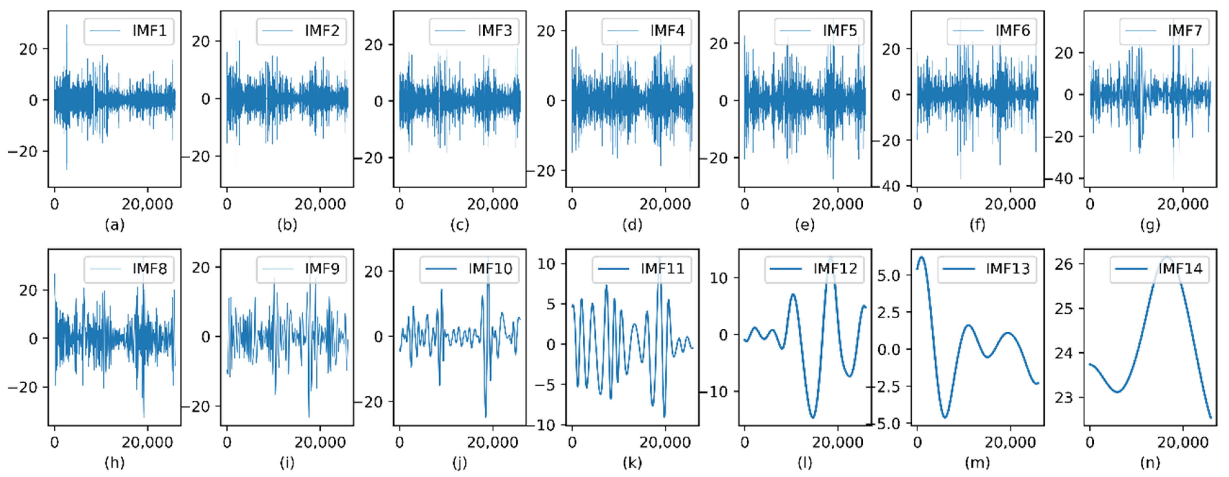
3.4.1. CEEMDAN Modal Decomposition
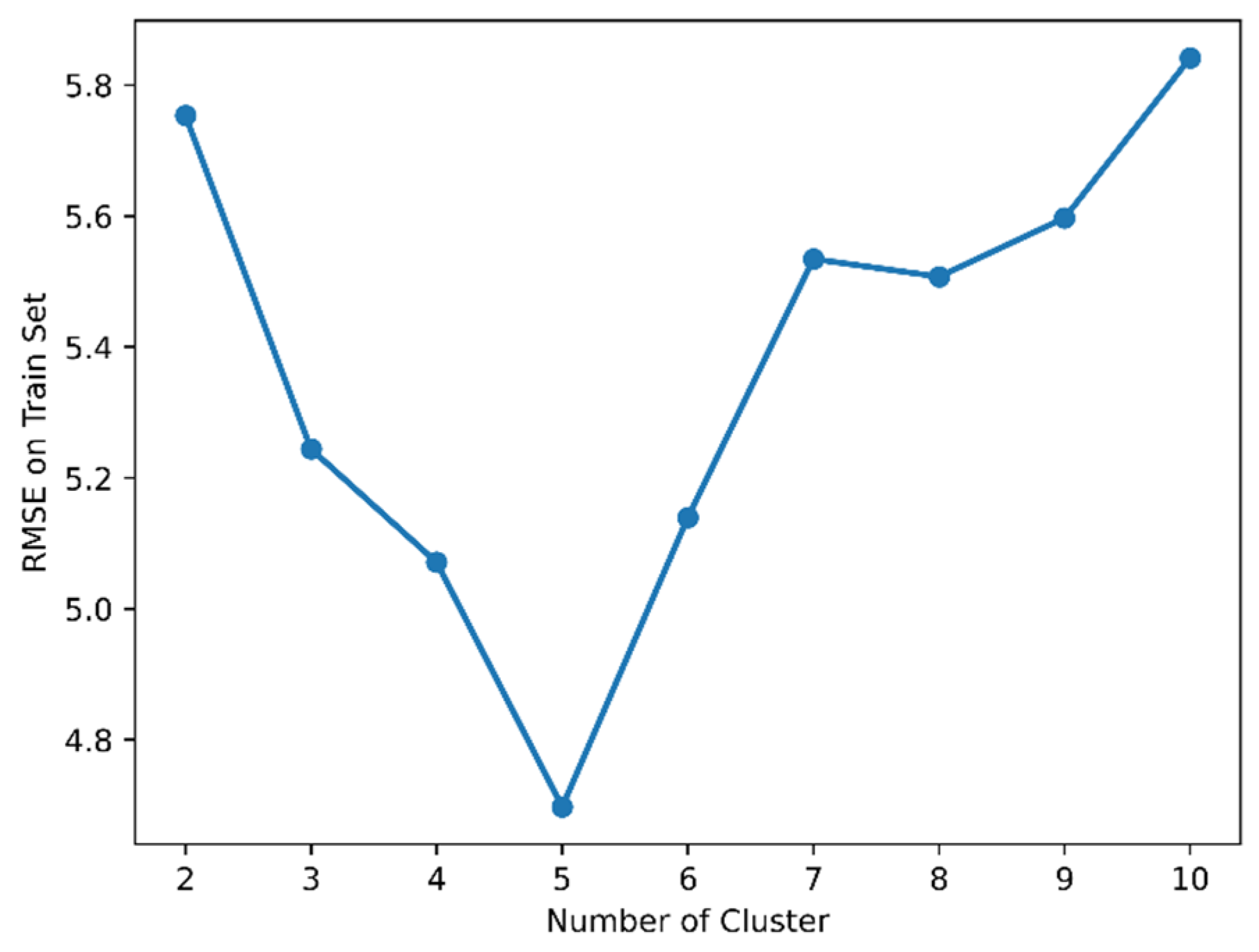
3.4.2. FE Calculation Results
3.4.3. BiLSTM Experiment Results
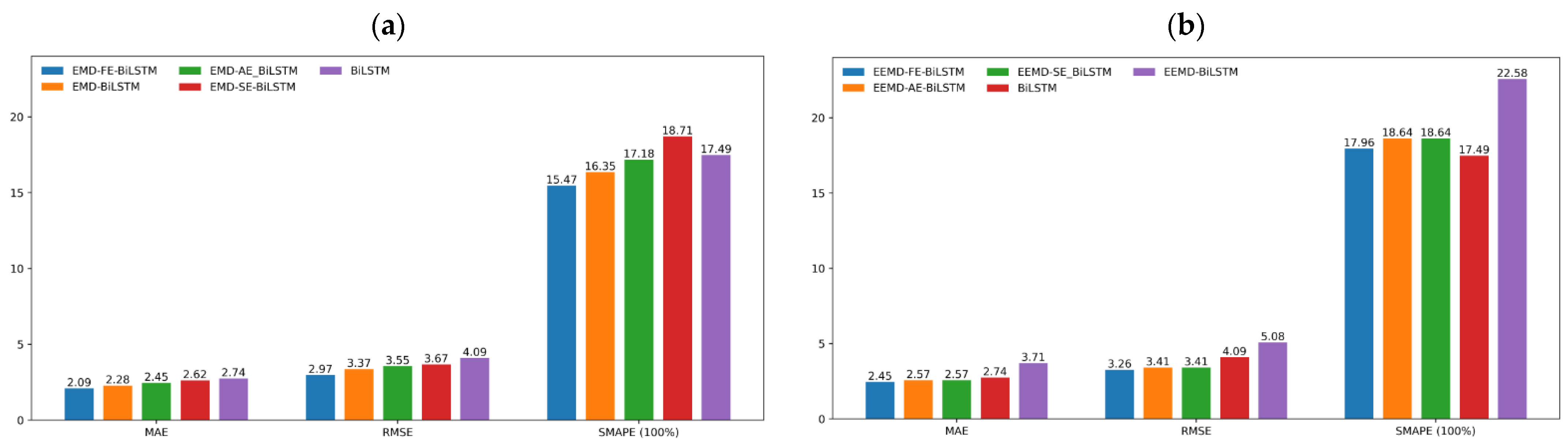
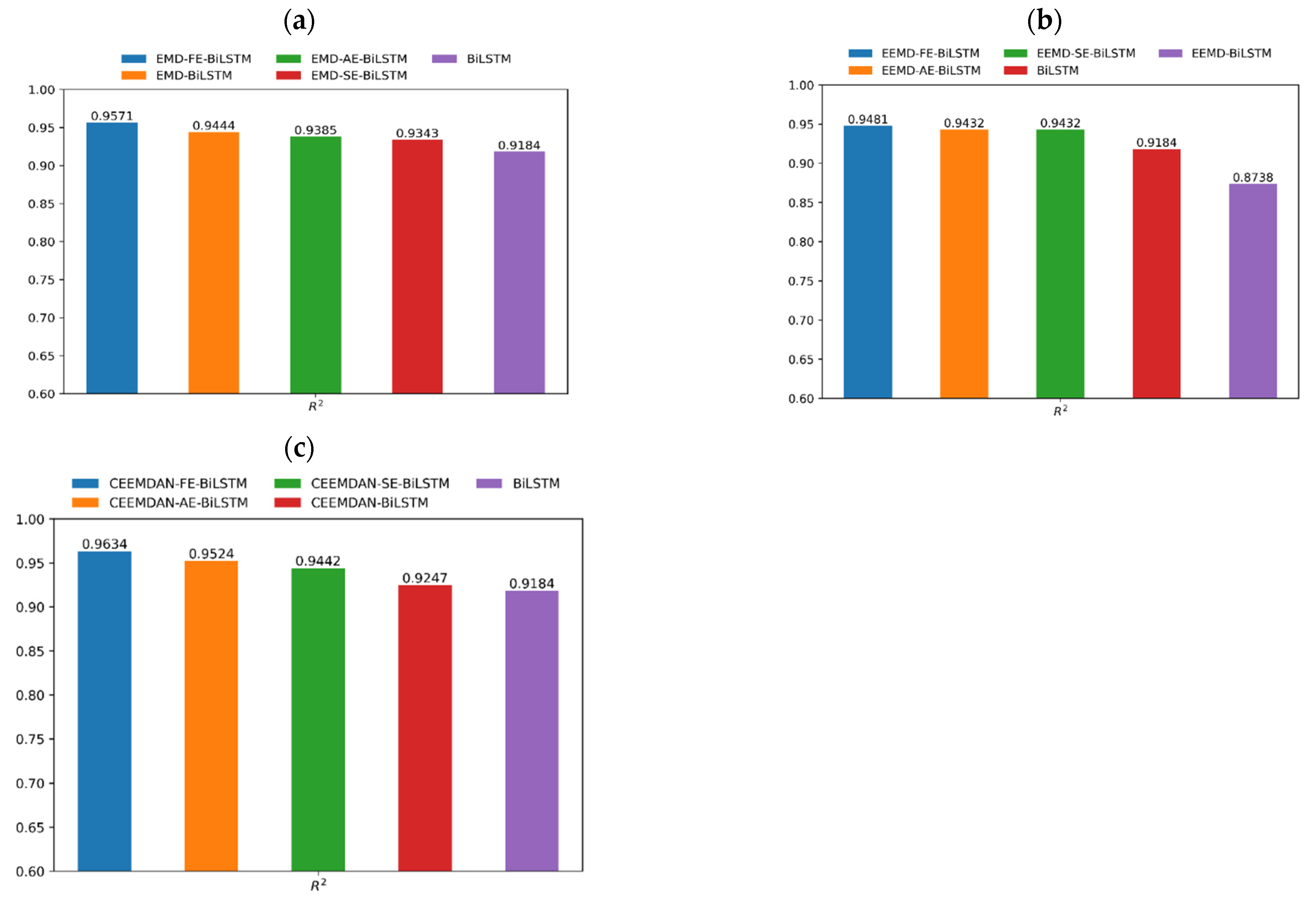
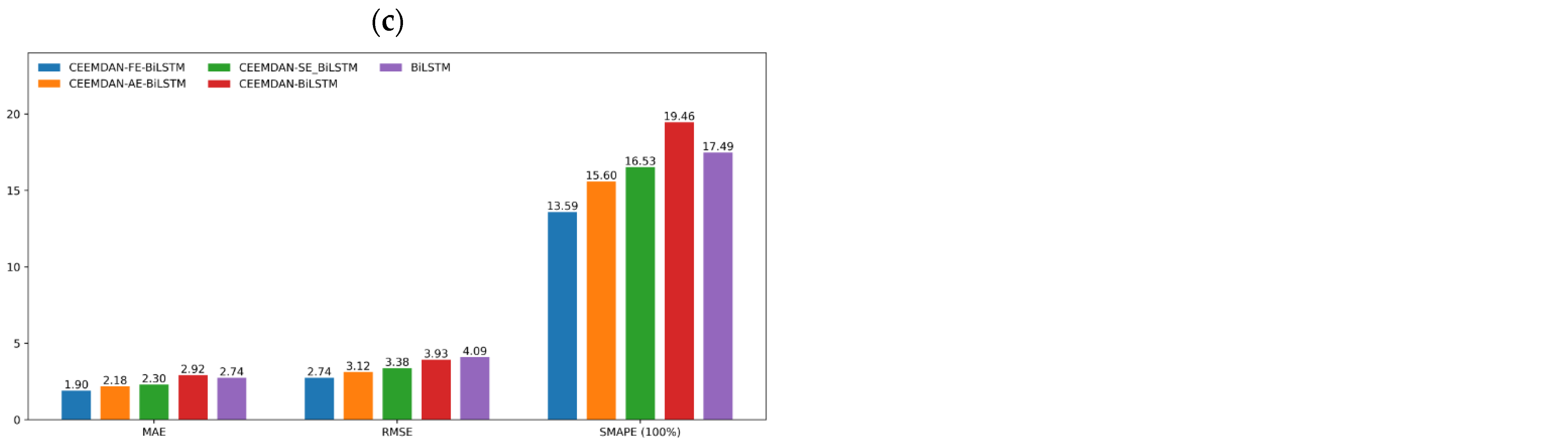
3.5. Model Comparison Analysis
4. Extension Analysis
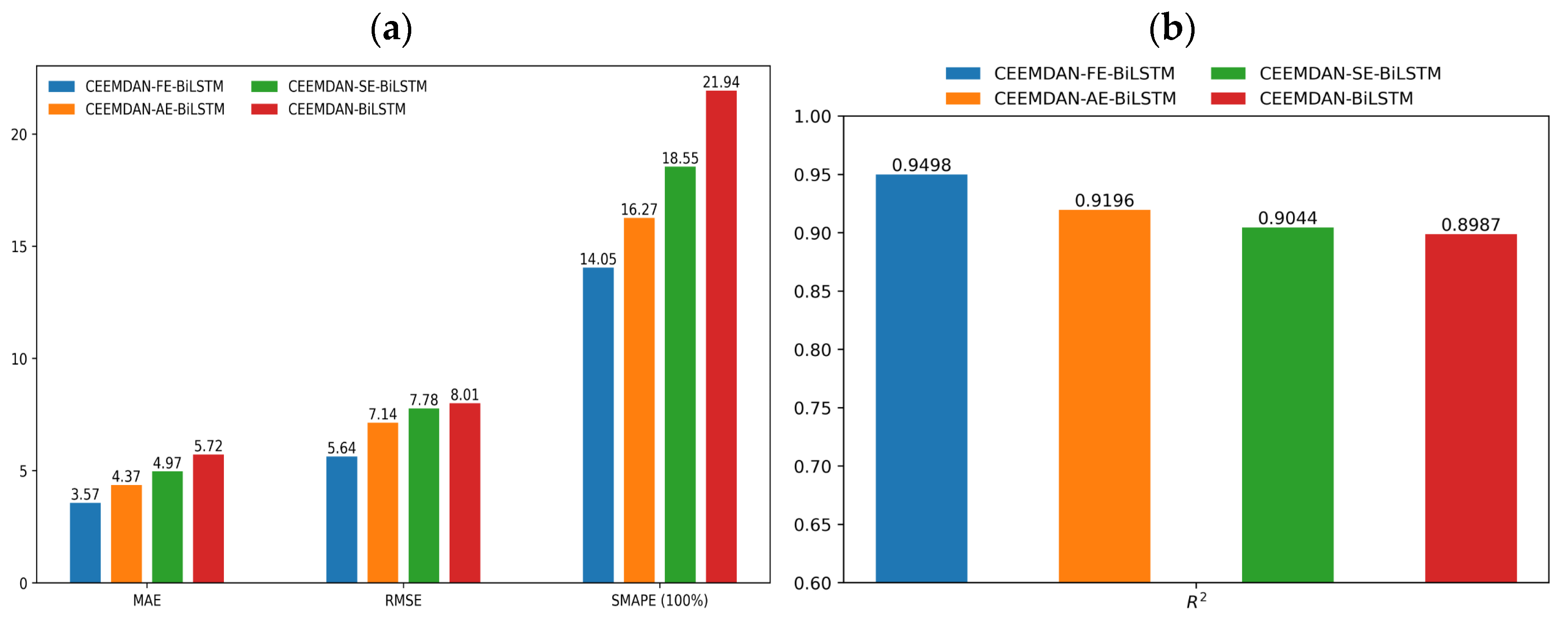
4.1. Predictive Analysis of PM10
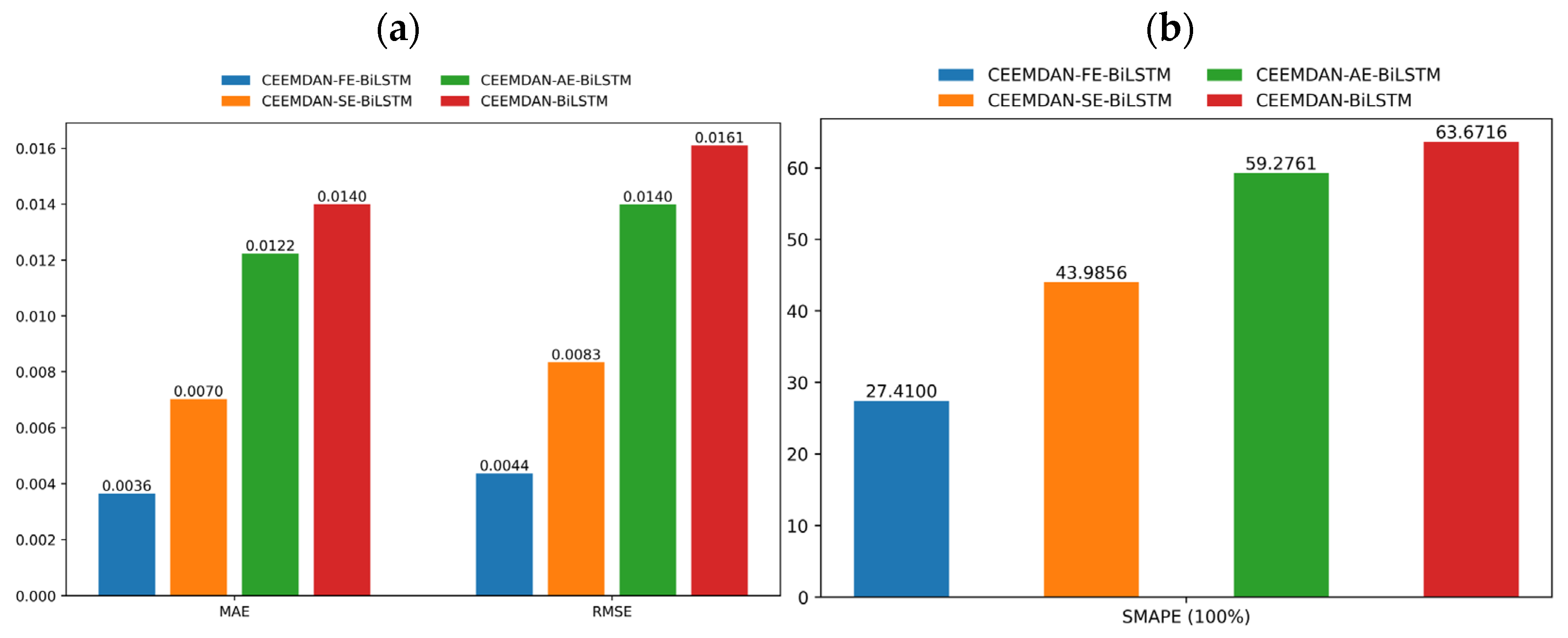
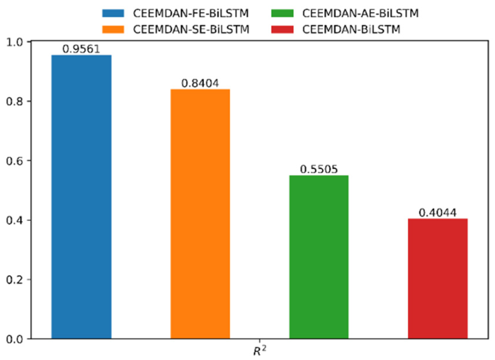
4.2. Predictive Analysis of O3
5. Conclusions
Author Contributions
Funding
Institutional Review Board Statement
Informed Consent Statement
Data Availability Statement
Conflicts of Interest
References
- Guérette, E.A.; Chang, L.T.C.; Cope, M.E.; Duc, H.N.; Emmerson, K.M.; Monk, K.; Rayner, P.J.; Scorgie, Y.; Silver, J.D.; Simmons, J. Evaluation of Regional Air Quality Models over Sydney, Australia: Part 2, Comparison of PM2.5 and Ozone. Atmosphere 2020, 11, 233. [Google Scholar] [CrossRef]
- Olukanni, D.; Enetomhe, D.; Bamigboye, G.; Bassey, D. A Time-Based Assessment of Particulate Matter (PM2.5) Levels at a Highly Trafficked Intersection: Case Study of Sango-Ota, Nigeria. Atmosphere 2021, 12, 532. [Google Scholar] [CrossRef]
- Yin, X.; Huang, Z.; Zheng, J.; Yuan, Z.; Zhu, W.; Huang, X.; Chen, D. Source contributions to PM2.5 in Guangdong province, China by numerical modeling: Results and implications. Atmos. Res. 2017, 186, 63–71. [Google Scholar] [CrossRef]
- Shoji, H.; Tsukatani, T. Statistical model of air pollutant concentration and its application to the air quality standards. Atmos. Environ. 1973, 7, 485–501. [Google Scholar] [CrossRef]
- Liu, J.; Weng, F.; Li, Z. Satellite-based PM2.5 estimation directly from reflectance at the top of the atmosphere using a machine learning algorithm. Atmos. Environ. 2019, 208, 113–122. [Google Scholar] [CrossRef]
- Altikat, S. Prediction of CO2 emission from greenhouse to atmosphere with artificial neural networks and deep learning neural networks. Int. J. Environ. Sci. Technol. 2021, 18, 3169–3178. [Google Scholar] [CrossRef]
- Choi, B.S. ARMA Model Identification; Springer Science & Business Media: Berlin/Heidelberg, Germany, 2012. [Google Scholar]
- Zhang, L.; Lin, J.; Qiu, R.; Hu, X.; Zhang, H.; Chen, Q.; Tan, H.; Lin, D.; Wang, J. Trend Analysis and Forecast of PM2.5 in Fuzhou, China Using the ARIMA Model. Ecol. Indic. 2018, 95, 702–710. [Google Scholar] [CrossRef]
- Venkataraman, V.; Usmanulla, S.; Sonnappa, A.; Sadashiv, P.; Mohammed, S.S.; Narayanan, S.S. Wavelet and multiple linear regression analysis for identifying factors affecting particulate matter PM2.5 in Mumbai City, India. Int. J. Qual. Reliab. Manag. 2019, 36, 1750–1783. [Google Scholar] [CrossRef]
- Zhou, Y.; Chang, F.J.; Chang, L.C.; Kao, I.F.; Wang, Y.S.; Kang, C.C. Multi-output Support Vector Machine for Regional Multi Step-ahead PM2.5 Forecasting. Sci. Total Environ. 2019, 651, 230–240. [Google Scholar] [CrossRef] [PubMed]
- Zaremba, W.; Sutskever, I.; Vinyals, O. Recurrent neural network regularization. arXiv 2014, arXiv:1409.2329. [Google Scholar]
- Graves, A. Long short-term memory. In Supervised Sequence Labelling with Recurrent Neural Networks; Springer: Berlin/Heidelberg, Germany, 2012; pp. 37–45. [Google Scholar]
- Dey, R.; Salem, F.M. Gate-variants of gated recurrent unit (GRU) neural networks. In Proceedings of the 2017 IEEE 60th International Midwest Symposium on Circuits and Systems (MWSCAS), Boston, MA, USA, 6–9 August 2017; IEEE: Piscataway, NJ, USA, 2017; pp. 1597–1600. [Google Scholar]
- Xiao, F.; Yang, M.; Fan, H.; Fan, G.; Al-Qaness, M.A. An improved deep learning model for predicting daily PM2.5 concentration. Sci. Rep. 2020, 10, 20988. [Google Scholar] [CrossRef]
- Al-Qaness, M.A.; Fan, H.; Ewees, A.A.; Yousri, D.; Abd Elaziz, M. Improved ANFIS model for forecasting Wuhan City air quality and analysis COVID-19 lockdown impacts on air quality. Environ. Res. 2021, 194, 110607. [Google Scholar] [CrossRef] [PubMed]
- Singh, S.; Parmar, K.S.; Kumar, J.; Makkhan, S.J.S. Development of new hybrid model of discrete wavelet decomposition and autoregressive integrated moving average (ARIMA) models in application to one month forecast the casualties cases of COVID-19. Chaos Soliton Fract. 2020, 135, 109866. [Google Scholar] [CrossRef] [PubMed]
- Singh, S.; Parmar, K.S.; Kumar, J.; Makkhan, S.J.S. A hybrid WA–CPSO-LSSVR model for dissolved oxygen content prediction in crab culture. Eng. Appl. Artif. Intell. 2014, 29, 114–124. [Google Scholar]
- Zheng, H.; Yuan, J.; Chen, L. Short-term load forecasting using EMD-LSTM neural networks with a Xgboost algorithm for feature importance evaluation. Energies 2017, 10, 1168. [Google Scholar] [CrossRef] [Green Version]
- Niu, M.F.; Gan, K.; Sun, S.L.; Li, F.Y. Application of decomposition-ensemble learning paradigm with phase space reconstruction for day-ahead PM2.5 concentration forecasting. J. Environ. Manag. 2017, 196, 110–118. [Google Scholar] [CrossRef]
- Kerui, W.; Miao, L.; Qian, L. An integrated prediction model of PM2.5 concentration based on TPE-XGBOOST and LassoLars. Syst. Eng. Theory Pract. 2020, 40, 748–760. [Google Scholar]
- Sun, W.; Li, Z. Hourly PM2.5 Concentration Forecasting Based on Mode Decomposition Recombination Technique and Ensemble Learning Approach in Severe Haze Episodes of China. J. Clean. Prod. 2020, 263, 121442. [Google Scholar] [CrossRef]
- Cao, J.; Li, Z.; Li, J. Financial time series forecasting model based on CEEMDAN and LSTM. Physica A 2019, 519, 127–139. [Google Scholar] [CrossRef]
- Rilling, G.; Flandrin, P.; Gonçalves, P.; Lilly, J.M. Bivariate empirical mode decomposition. IEEE Signal. Proc. Lett. 2007, 14, 936–939. [Google Scholar] [CrossRef] [Green Version]
- Wu, Z.H.; Huang, N.E. Ensemble empirical mode decomposition: A noise-assisted data analysis method. Adv. Adapt. Data Anal. 2009, 1, 1–41. [Google Scholar] [CrossRef]
- Tran, D.; Wagner, M. Fuzzy entropy clustering. In Proceedings of the Ninth IEEE International Conference on Fuzzy Systems, San Antonio, TX, USA, 7–10 May 2000; FUZZ-IEEE 2000 (Cat. No. 00CH37063). IEEE: Piscataway, NJ, USA, 2000; Volume 1, pp. 152–157. [Google Scholar]
- Yentes, J.M.; Hunt, N.; Schmid, K.K.; Kaipust, J.P.; McGrath, D.; Stergiou, N. The appropriate use of approximate entropy and sample entropy with short data sets. Ann. Biomed. Eng. 2013, 41, 349–365. [Google Scholar] [CrossRef] [PubMed]
- Wang, D.; Zhong, J.; Shen, C.; Pan, E.; Peng, Z.; Li, C. Correlation dimension and approximate entropy for machine condition monitoring: Revisited. Mech. Syst. Signal. Process. 2021, 152, 107497. [Google Scholar] [CrossRef]
- Hochreiter, S.; Schmidhuber, J. Long short-term memory. Neural Comput. 1997, 9, 1735–1780. [Google Scholar] [CrossRef] [PubMed]
- Gers, F.A.; Jürgen, S.; Cummins, F. Learning to Forget: Continual Prediction with LSTM. Neural Comput. 2000, 12, 2451–2471. [Google Scholar] [CrossRef]
- Schuster, M.; Paliwal, K.K. Bidirectional recurrent neural networks. IEEE Trans. Signal. Process. 1997, 45, 2673–2681. [Google Scholar] [CrossRef] [Green Version]
- Li, J.; Li, D.C. Short-term wind power forecasting based on CEEMDAN-FE-KELM method. Inf. Control 2016, 45, 135–141. [Google Scholar]


| Main Hyperparameter | Set Value |
|---|---|
| Batch size | 12 |
| Number of hidden layer units | 32 |
| Hidden layers | 2 |
| Learning rate | 5 × 10⁻³ |
| Max epoch | 30 |
| Optimizer | Adam |
| Loss function | MSE |
| Decomposition Sequence IMFi | FE Value | Decomposition Sequence IMFi | FE Value |
|---|---|---|---|
| IMF1 | 2.610 | IMF8 | 0.424 |
| IMF2 | 2.463 | IMF9 | 0.160 |
| IMF3 | 1.884 | IMF10 | 0.038 |
| IMF4 | 1.275 | IMF11 | 0.006 |
| IMF5 | 0.915 | IMF12 | 0.001 |
| IMF6 | 0.704 | IMF13 | 7.40 × 10⁻⁵ |
| IMF7 | 0.578 | IMF14 | 4.82 × 10⁻⁶ |
| Models | RMSE | MAE | SMAPE | R2 |
|---|---|---|---|---|
| BiLSTM | 4.09 | 2.74 | 17.49% | 91.84% |
| EMD-BiLSTM | 3.37 | 2.28 | 16.35% | 94.44% |
| EMD-SE-BiLSTM | 3.67 | 2.62 | 18.71% | 93.43% |
| EMD-AE-BiLSTM | 3.55 | 2.45 | 17.18% | 93.85% |
| EMD-FE-BiLSTM | 2.97 | 2.09 | 15.47% | 95.71% |
| EEMD-BiLSTM | 5.08 | 3.71 | 22.58% | 87.38% |
| EEMD-SE-BiLSTM * | 3.41 | 2.57 | 18.64% | 94.32% |
| EEMD-AE-BiLSTM * | 3.41 | 2.57 | 18.64% | 94.32% |
| EEMD-FE-BiLSTM | 3.26 | 2.45 | 17.96% | 94.81% |
| CEEMDAN-BiLSTM | 3.93 | 2.92 | 19.46% | 92.47% |
| CEEMDAN-SE-BiLSTM | 3.38 | 2.30 | 16.53% | 94.42% |
| CEEMDAN-AE-BiLSTM | 3.12 | 2.18 | 15.60% | 95.24% |
| CEEMDAN-FE-BiLSTM | 2.74 | 1.90 | 13.59% | 96.34% |
| Model | RMSE | MAE | SMAPE | R2 |
|---|---|---|---|---|
| CEEMDAN-BiLSTM | 8.01 | 5.72 | 21.94% | 89.87% |
| CEEMDAN-SE-BiLSTM | 7.78 | 4.97 | 18.55% | 90.44% |
| CEEMDAN-AE-BiLSTM | 7.14 | 4.37 | 16.27% | 91.96% |
| CEEMDAN-FE-BiLSTM | 5.64 | 3.57 | 14.05% | 94.98% |
| Model | RMSE | MAE | SMAPE | R2 |
|---|---|---|---|---|
| CEEMDAN-BiLSTM | 0.0161 | 0.0140 | 63.67% | 40.44% |
| CEEMDAN-SE-BiLSTM | 0.0083 | 0.0070 | 43.99% | 84.04% |
| CEEMDAN-AE-BiLSTM | 0.0140 | 0.0122 | 59.28% | 55.05% |
| CEEMDAN-FE-BiLSTM | 0.0044 | 0.0036 | 27.41% | 95.61% |
Publisher’s Note: MDPI stays neutral with regard to jurisdictional claims in published maps and institutional affiliations. |
© 2021 by the authors. Licensee MDPI, Basel, Switzerland. This article is an open access article distributed under the terms and conditions of the Creative Commons Attribution (CC BY) license (https://creativecommons.org/licenses/by/4.0/).
Share and Cite
Jiang, X.; Wei, P.; Luo, Y.; Li, Y. Air Pollutant Concentration Prediction Based on a CEEMDAN-FE-BiLSTM Model. Atmosphere 2021, 12, 1452. https://doi.org/10.3390/atmos12111452
Jiang X, Wei P, Luo Y, Li Y. Air Pollutant Concentration Prediction Based on a CEEMDAN-FE-BiLSTM Model. Atmosphere. 2021; 12(11):1452. https://doi.org/10.3390/atmos12111452
Chicago/Turabian StyleJiang, Xuchu, Peiyao Wei, Yiwen Luo, and Ying Li. 2021. "Air Pollutant Concentration Prediction Based on a CEEMDAN-FE-BiLSTM Model" Atmosphere 12, no. 11: 1452. https://doi.org/10.3390/atmos12111452
APA StyleJiang, X., Wei, P., Luo, Y., & Li, Y. (2021). Air Pollutant Concentration Prediction Based on a CEEMDAN-FE-BiLSTM Model. Atmosphere, 12(11), 1452. https://doi.org/10.3390/atmos12111452