Article

A System to Improve Port Navigation Safety and Its Use in Italian Harbours

by
Maurizio Soldani
1,* and
Osvaldo Faggioni
1,2
1
Istituto Nazionale di Geofisica e Vulcanologia, Via di Vigna Murata 605, 00143 Roma, Italy
2
Department of Electric, Electronic, Telecommunication Engineering and Naval Architecture, University of Genoa, Via all’Opera Pia 11A, 16145 Genova, Italy
*
Author to whom correspondence should be addressed.
Appl. Sci. 2021, 11(21), 10265; https://doi.org/10.3390/app112110265
Submission received: 28 September 2021 / Revised: 22 October 2021 / Accepted: 25 October 2021 / Published: 1 November 2021

Abstract

:
This article describes research aimed at developing a system able to support local authorities and port communities in optimizing port navigation, avoiding or managing critical situations induced by sea-level variations in harbours and minimizing environmental damages and economic losses. In the Mediterranean basin, sea-level changes are mostly due to astronomical tides, related to the gravitational attraction between Earth, Moon and Sun. Nevertheless, sea-level variations are also influenced by meteorological tides, which are geodetic adjustments of sea surface due to atmospheric pressure variations above a water basin. So, starting from monitoring or forecasting environmental parameters in harbours, the system updates port bathymetric maps based on sea-level variations (acquired in the past, measured in real-time, or expected in the future) and detects hazardous areas for a certain ship moving inside a port at a given moment, by means of the implementation of “virtual traffic lights”. The system was tested on some real situations, including the analysis of maritime accidents (stranding of ships), providing satisfactory results by correctly signalling potentially dangerous areas variable over time. The architecture of the system and results achieved using it in the ports of Livorno and Bari, in Italy, are herewith described.

1. Introduction

Sea level variations in coastal areas affect—in a relevant way—the safety of people working on ports. In fact, these phenomena influence the so-called harbour waterside management (optimization of maritime transport, dock performances, vessel mooring, logistics operations, ship loading, maritime works, marine water quality and pollution control). Therefore, their knowledge and forecasting can be very useful in order to minimize the risk of accidents (e.g., stranding of ships) and the consequent environmental impact and economic losses [1,2,3,4,5,6,7,8,9,10,11,12,13,14,15,16,17,18,19,20].
The system described in this article starts from monitoring (or forecasting) sea level and meteorological parameters (mainly the atmospheric pressure) in harbours; then, sea-level values acquired or expected are passed as inputs to a software application which updates the bathymetric map of a basin and detects potentially dangerous situations for a certain ship at a given instant, with the aim of supporting local authorities and working organizations in optimizing harbour water management and port operations, mitigating risk due to sea-level variations and managing emergencies.
The software tool is able to update in real-time the bathymetric map of a harbour by downloading via Internet sea-level data acquired by meteo-mareographic stations working in ports; it can also read data stored in an archive to replicate the evolution of the bathymetry in the occasion of remarkable events occurred in the past, such as ship stranding or refloating; finally, as explained below, it is also able to make use of atmospheric pressure trends to estimate future sea-level changes named meteorological tides, which have to be added to the astronomical ones, that are periodic and well-known, to obtain the expected sea level and then the future real bathymetric map of a port.
In fact, the slow up-down motion of sea level in Mediterranean coastal areas is essentially due to tides that are mainly the sum of astronomical components (in particular the diurnal and the semidiurnal ones) due to gravitational attraction between Earth, Moon and Sun, and then periodic, well-known (through harmonic analysis) and foreseeable for each location by means of tide charts [21].
In addition to them, an important role in determining tidal fluctuations can be played by meteorological components (due to atmospheric pressure perturbations), in particular, if they occur along with the astronomical ones. During the last ten years, “anomalous” tidal oscillations have been observed along Italian coasts. In particular, a meteorological tide (also named “meteo-tide”) is a geodetic adjustment of the sea surface resulting from a perturbation of atmospheric weight above a water basin (up and down sea level motion that compensates the Newtonian unbalance): an increase in atmospheric loading induces an outcoming seawater flux (low tide), while a decrease in atmospheric weight causes an incoming flux (high tide); therefore, sea level lowers with an atmospheric pressure rise, and rises with a pressure fall. This phenomenon depends on a lot of variables (e.g., the topography of the basin) so, unlike the previous phenomenon, it is not describable by a deterministic law: the statistical correlation between changes of atmospheric pressure (cause) and sea-level variations (effect) is estimated by analysing meteorological events (sea-level changes consequent to atmospheric pressure variations) that occur in a certain location for a long time interval. Once this correlation (named hydro-barometric transfer factor) is known, meteorological tides can be forecasted starting from the knowledge of atmospheric pressure variations [22,23,24,25,26,27,28,29,30].
Finally, once astronomical and meteorological tides are both known, the expected global variation of sea level can be estimated as the algebraic sum of the two contributions and then passed as input to the software application that performs the updating of the bathymetry.
Here. we describe the results obtained by using this system in real situations in Livorno and Bari harbours, in Italy (see Figure 1).

2. Materials and Methods

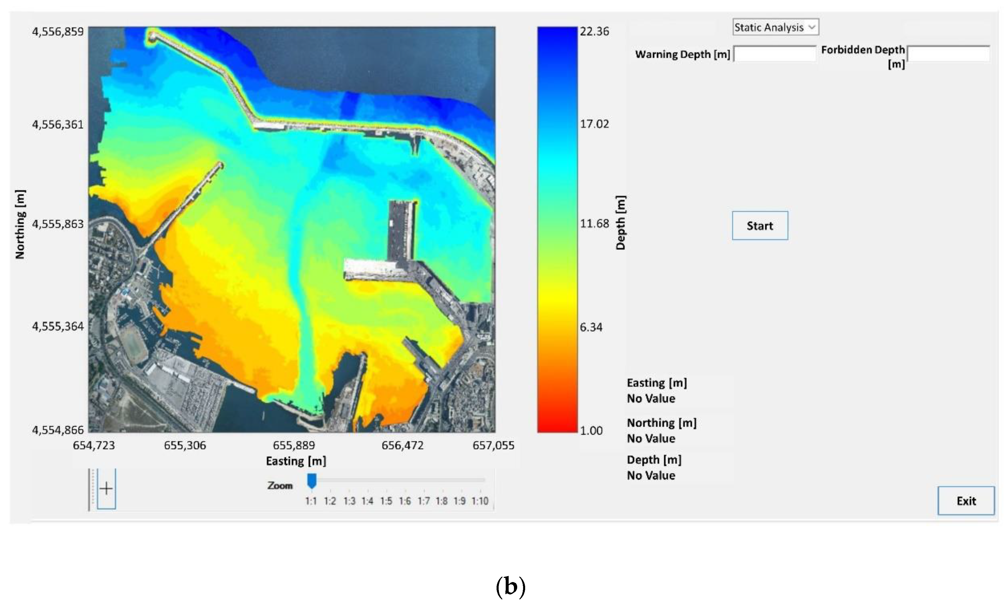
2.1. Bathymetry Updating and “Virtual Traffic Lights”

Here, we describe the software tool developed to update automatically the bathymetry of a basin (based on sea level measured or forecasted) and to implement the idea of virtual traffic lights (by means of comparison with two threshold levels); this represents a helpful graphical interface to support authorities in avoiding or managing critical situations by detecting hazardous areas [31,32,33,34,35,36,37,38,39].
The initial condition (referred to time t0) of the processing procedure is the georeferenced bathymetric map of a port as it usually results from multibeam surveys; this represents the static bathymetry because it changes only after a new survey following variations of the basin topography, for instance, due to dredging operations or natural phenomena such as coastal erosion, sediment deposit, sea bottom subsidence.
Figure 2a represents the bathymetric map of the port of Livorno, that extends over an area of approximately 18 [km2]; the grid spacing is equal to 5 [m]; the coordinates are represented in UTM (Universal Transverse of Mercator coordinates, Zone 32T) and bottom depth values are referred to IGM’s 0 sea level (Italian Military Geographic Institute) with a resolution of 10−2 [m]. On the contrary, Figure 2b shows the map of Bari harbour (area of about 4.8 [km2]; spatial resolution 1 [m]; UTM Zone 33T); bathymetric data have been kindly provided by Port Authorities of Livorno and Bari.
It is possible to set two thresholds, a lower and an upper level, variable from ship to ship depending on the draught of the vessel under monitoring, to divide the bathymetry into different areas represented by three colours: seafloor depth values smaller than the lower threshold (usually set equal to the vessel draught) identify zones that are forbidden for that vessel and are represented by red colour, while depth values greater than the upper threshold identify deep or allowed zones (green: bottom depth more than the upper threshold, in its turn greater than the ship draught: there is a wide under-keel clearance (the space between the lowest point of the vessel keel and the sea bottom under it)); finally, depth values between lower and upper values identify shallow or warning zones (yellow: a gradual transition from the green area to the red one, with bottom depth values between the lower threshold and the upper one: there is a little space between the vessel keel and the seafloor). The partition of the harbour area into three different colours shows prohibited, allowed or warning zones for that vessel and so it implements the idea of virtual traffic lights customized for each ship: in a hypothetical operational scenario, the choice of thresholds would be a task of end users (port communities).
For example, regarding the port of Livorno, for a ship having a draught of 10 m thresholds could be set at 10 and 11 m, respectively; it follows the representation shown in Figure 3a: therefore, for that ship, we consider as forbidden (red) the areas with bottom depth less than 10 m, warning areas (yellow) those in which the depth is between 10 and 11 m, and allowed areas (green) those where the depth is greater than 11 m. This is the so-called static analysis (the map does not change over time). In Figure 3b the same map is shown but after different thresholds have been chosen: for a hypothetical ship with a greater draught than the previous case, e.g., 11.5 m, choosing threshold levels set at 11.5 and 12.5 m, respectively, leads to expand the red (prohibited) zone and to reduce the green (allowed) area: we consider as forbidden the zones with a seafloor depth of less than 11.5 m, warning areas those with a depth between 11.5 and 12.5 m, and allowed areas those with a depth greater than 12.5 m; obviously, for a ship with a deeper draught, a larger (red) area will be forbidden.
In Figure 4 the bathymetric map of Bari harbour is represented, with threshold levels equal to 8 and 9 m in Figure 4a and 9 and 10 m in Figure 4b.
After this, sea level values can be added to the starting bottom depth to recalculate moment by moment the georeferenced bathymetric map and update the so-called dynamic bathymetry (variable over time). Mareographic signals can represent past measurements loaded from a dataset (to analyse bathymetry variations during past events of particular interest, e.g., vessel stranding or refloating) or real-time values transmitted by monitoring stations described in the Section 2.2 (if we are observing the real-time evolution of the bathymetry), but it is also possible to load expected sea-level values resulting from the forecasting procedure described later in the Section 2.3, in order to forecast a future bathymetric map.
Then, the division of the port map into green, yellow and red areas is updated maintaining the same threshold levels (e.g., for the same vessel considered in Figure 4b, threshold levels remain constant at 9 and 10 m). Therefore, by varying sea level, an area that initially was prohibited (red), can become a warning (yellow) or allowed area (green) for that vessel, or vice versa. This represents the so-called dynamic analysis, because the real bathymetry varies over time, based on sea-level values loaded.
The processing procedure and the graphical interface of the application, running under the Windows operating system, have been developed using the C# language. Figure 5 shows the block diagram of the algorithm.

2.2. Environmental Monitoring in Harbours

To perform environmental monitoring in Italian harbours, meteo-mareographic stations belonging to the National Tidegauge Network managed by ISPRA (Italian Institute for Environmental Protection and Research) are usually employed. Regarding this work, parameters have been acquired by the ISPRA’s measurement stations located in the ports of Livorno and Bari (see Figure 6 and Figure 7).
A typical measurement station includes several instruments to measure environmental parameters, and among them, the most important for the study described in this article are the hydrometer to acquire sea level and the barometer to measure atmospheric pressure; it is also equipped with a data acquisition system, an Internet connection and a solar panel to provide the power supply.
Sea level measurements are usually referred to IGM’s 0 level. Their typical resolution is 10−2 m. The hydrometer essentially consists of a radar transducer positioned above the sea surface. Microwave pulses are sent towards the water/air interface, then, since the speed of the electromagnetic radiation in the air, the time taken by the impulses on the round trip, and the position of the transducer with respect to IGM’s 0 level are known, the sea level value is calculated. A typical sampling interval to acquire tide data is greater than or equal to 10 min and, to avoid the disturbance induced by sea waves, the radar transducer is usually placed inside a still-pipe.
The atmospheric pressure, on the contrary, is measured by means of a barometer based on a capacitive silicon transducer. As the atmospheric pressure varies, both distances between the two plates and electrical capacitance change; measurements are usually made once every hour (atmospheric pressure is characterized by very low-frequency variations), with a typical resolution equal to 10−1 hPa (1 hPa is approximately equal to 1 mbar).
The date and the time of a monitoring station are usually referred to as UTC—Universal Time Coordinates.
Data acquired can be stored in a memory (to create a local data archive), downloaded in real-time via the Internet on a receiving station (e.g., to implement a remote data storage or to update the bathymetric map of the port), and made available on a website. Data shown in this work and other information regarding the measurement stations are available on https://www.mareografico.it/ (accessed on 25 October 2021).

2.3. Forecasting Sea Level in Harbours

Meteo-tides are well-known in off-shore areas (the “inverted barometer” effect), where 1 hPa of atmospheric pressure change (cause) induces nearly 1 cm of sea-level variation (effect), but they need more study in coastal areas, where the shoreline prevents the displacement of the marine water mass along horizontal directions towards the coastline: the effect of this constraint is to amplify the vertical movement [40,41,42,43,44,45,46,47,48,49,50,51,52,53,54,55,56,57,58,59,60,61,62].
Moreover, the correlation between atmospheric pressure and sea level (represented by means of the so-called hydrobarometric transfer factor Jph) depends on a number of specific parameters for the location examined (overall the topography of the basin), therefore it cannot be described by means of a deterministic law valid everywhere but must be studied through a local observation of the phenomenon and subsequent statistical analysis. Therefore, the study of meteorological tides consists essentially in analysing events (sea-level variations consequent to atmospheric pressure changes) that occur in a given basin during a certain time interval (usually some years), to estimate the hydrobarometric transfer factor J
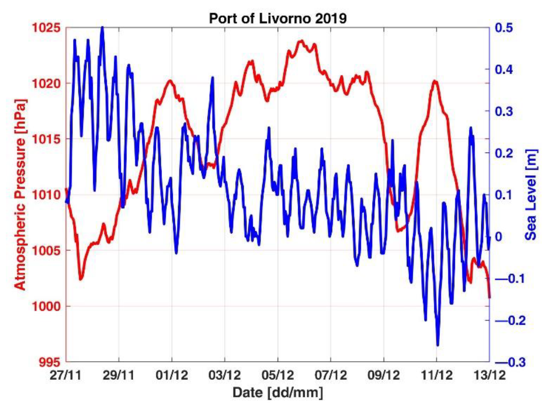
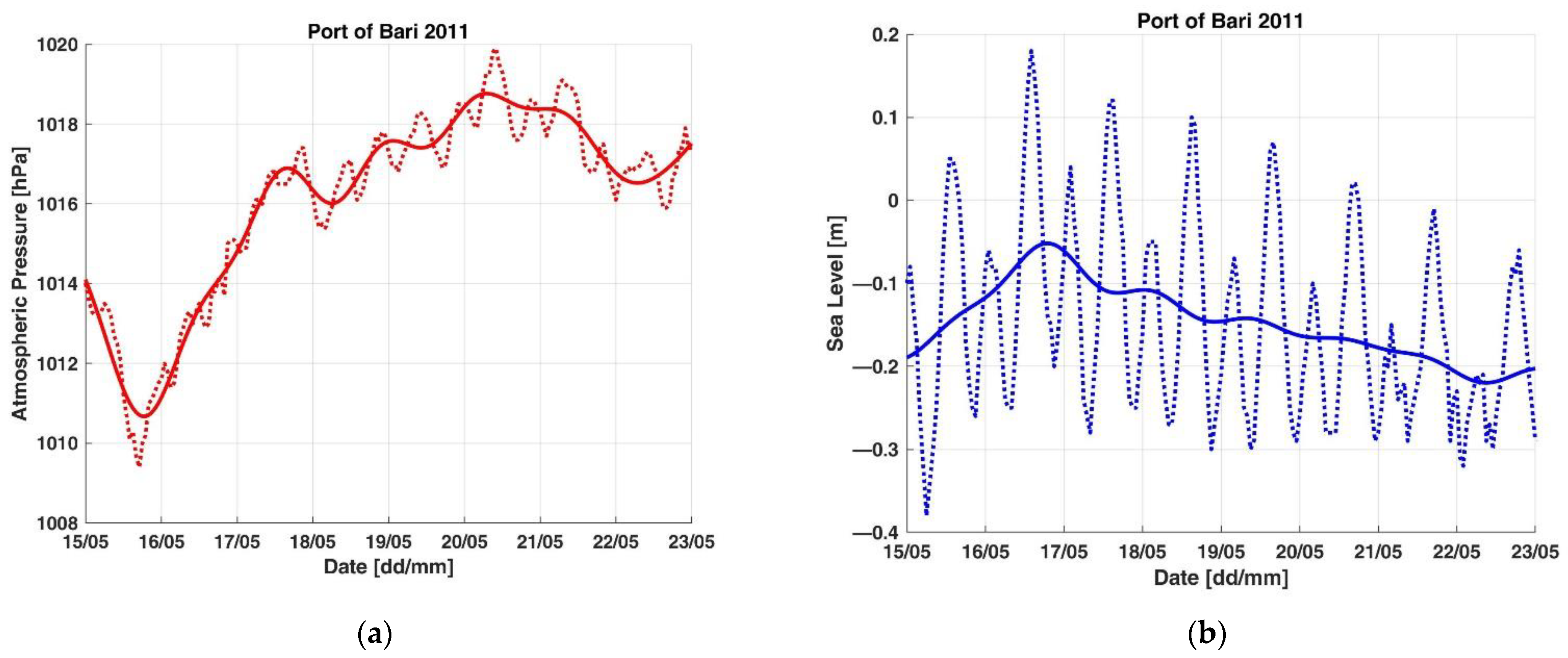
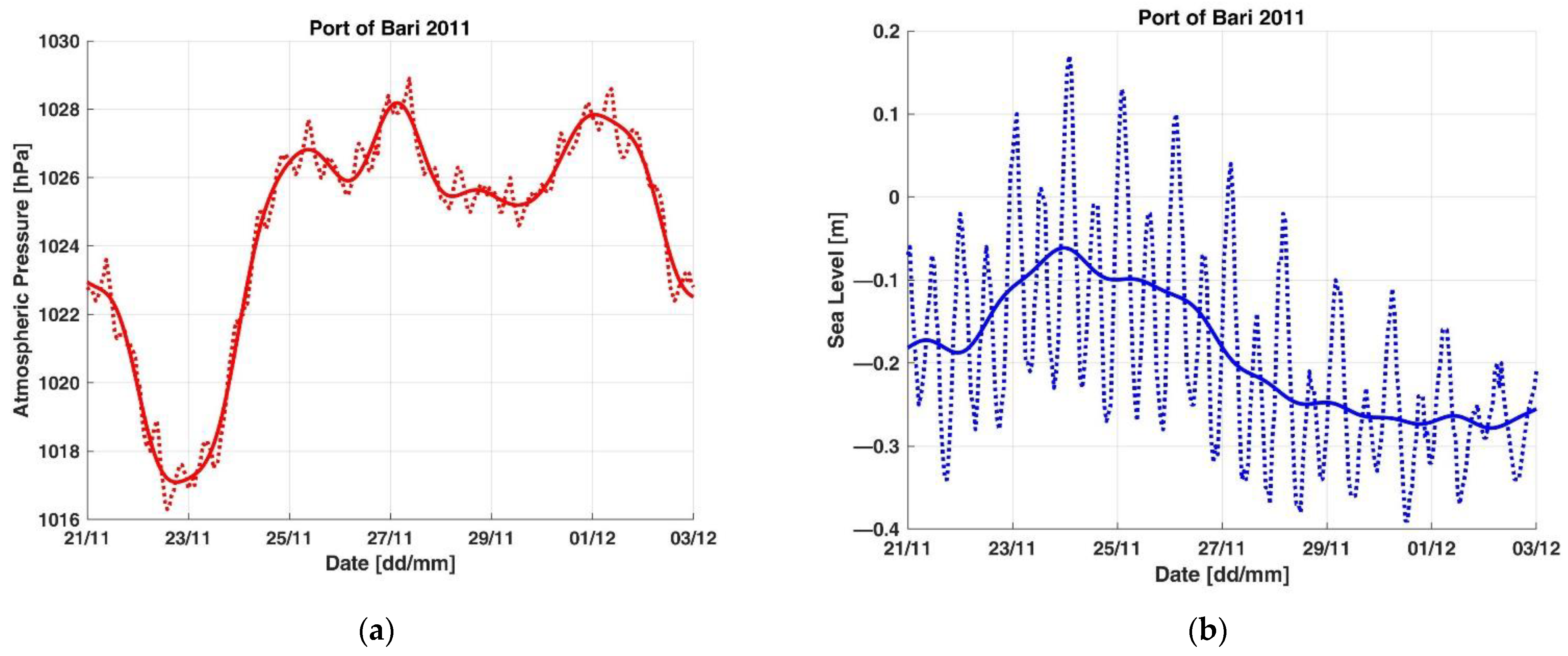
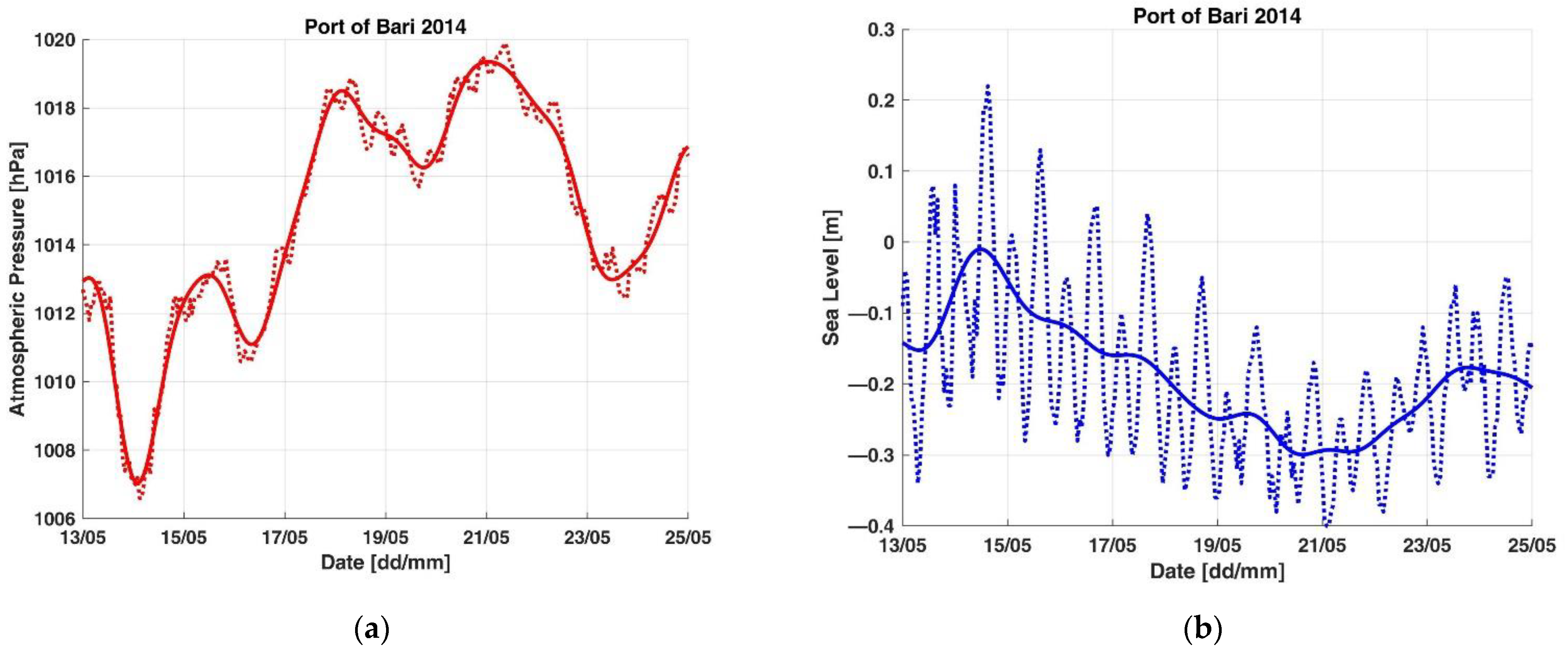
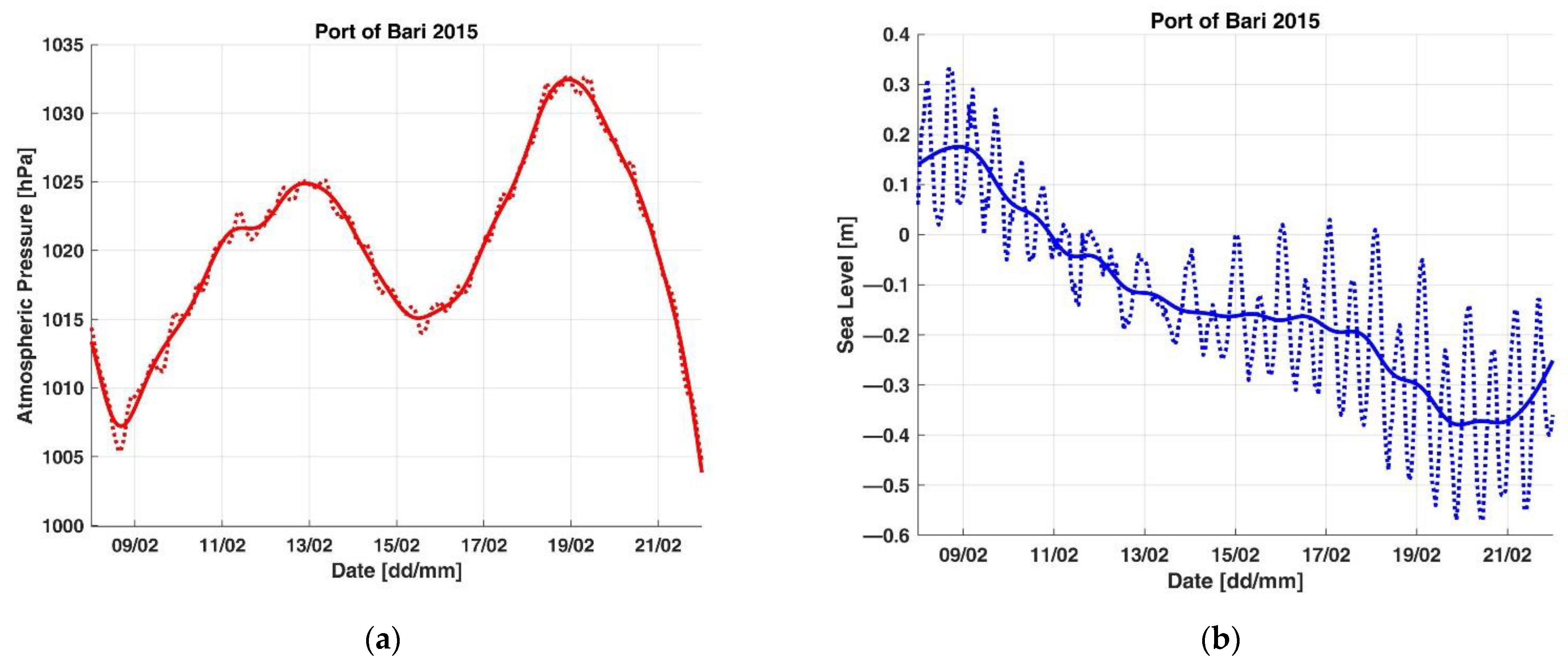
ph; the starting point is the monitoring of atmospheric pressure and sea level; for example, in Figure 8 parameters observed in the port of Livorno from 27 November to 13 December 2019 are shown, while Figure 9 refers to data acquired in Bari harbour from 15 to 23 May 2011.
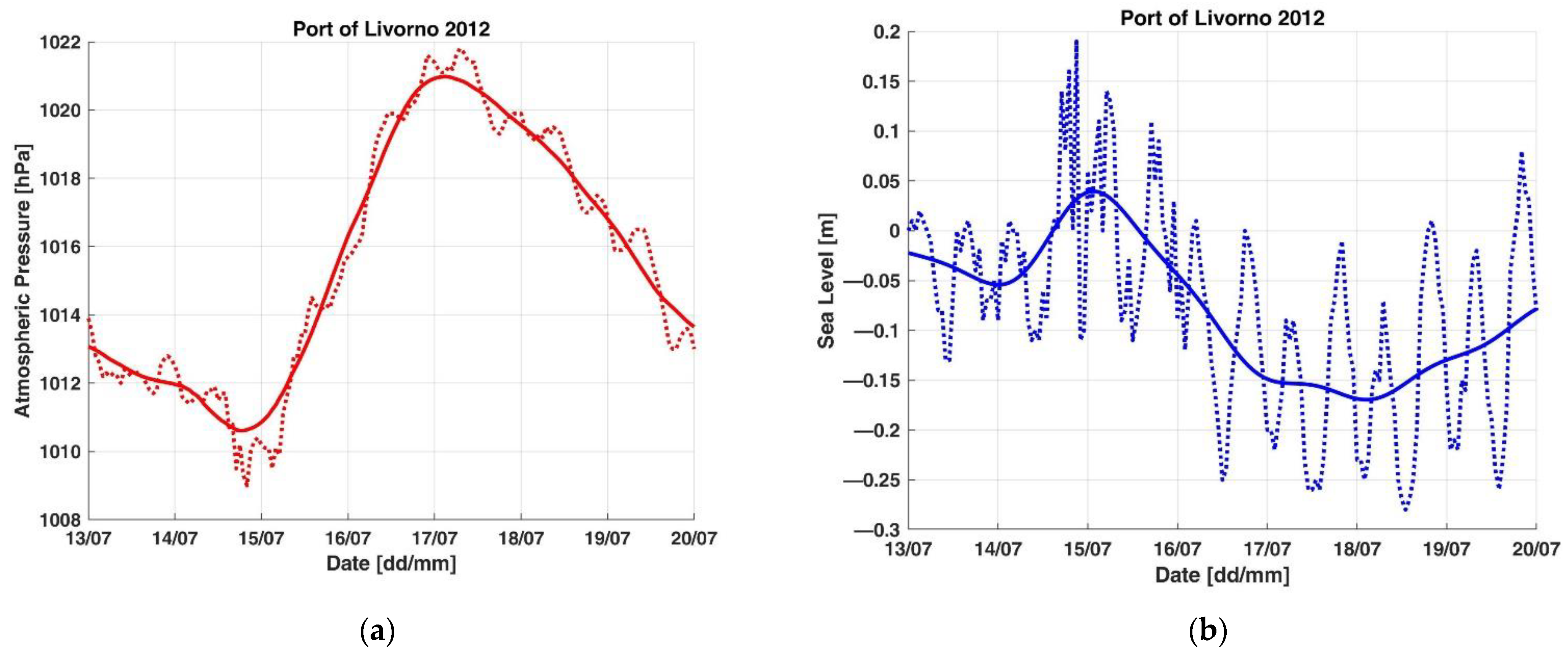
Sea level acquired includes all the phenomena that contribute to its variations, above all astronomical (in particular diurnal and semidiurnal) and meteorological tides. Other short-term phenomena such as wind effect and storm surges are not taken into consideration in this study (only events occurring in the absence of wind were studied). To remove contributions different from the meteorological one, measurements are filtered appropriately taking advantage of the fact that astronomical tides are characterized by high frequencies; power spectral densities of atmospheric pressure and sea level acquired in the port of Livorno during 2019 are shown in Figure 10: frequency components related to diurnal and semidiurnal tides are at about 1.2 and 2.3 · 10−5 Hz, respectively; Figure 11 shows the same quantities relating to the port of Bari in 2011.
Data are subjected to a Low Pass filtering that avoids diurnal and semidiurnal tides, which are the spectral components dashed in Figure 10, Figure 11, Figure 12 and Figure 13: only low-frequency components (slow variations), related to atmospheric pressure, survive the filtering (solid lines).
Regarding the period from 27 November to 13 December 2019 in Livorno, the filtered data shown in Figure 12 result, in which 19.5 hPa of atmospheric pressure increase in Δp (cause) induce nearly 45.2 cm of low meteorological tide Δh (height of tide wave, effect). As for filtered data from 15 to 23 May 2011 in Bari, Figure 13 shows that an increase in Δp of 8.1 hPa in atmospheric pressure causes a decrease in Δh of nearly 16.8 cm in sea level.
The hydrobarometric transfer factor Jph [cm·hPa−1] is estimated for each event as:
Jph = Δh/Δp,
expressed in absolute value, where Δh and Δp represent the change in sea level and atmospheric pressure, respectively; in these cases, we obtain a value of about 2.3 cm·hPa−1 for the event in Figure 12 and 2.1 cm·hPa−1 for the event in Figure 13.
In the ports of Livorno and Bari and, more in general, in Italian coastal areas, typical values found by means of a multi-year statistical analysis carried out for Jph are larger (even more than double) compared to the typical 1 cm·hPa−1 of the offshore; this phenomenon, if in phase with astronomical tides, can cause exceptional tide waves.
Then, for each event that happened in a given location in the period under consideration, the variation of low frequencies sea level Δh and the gradient of atmospheric pressure Δp are evaluated, and the calculation of Jph is repeated. Many pairs (Δp, Δh) and of corresponding values of Jph are obtained in this way, one for each occurrence of the phenomenon in the time interval examined in a certain basin.
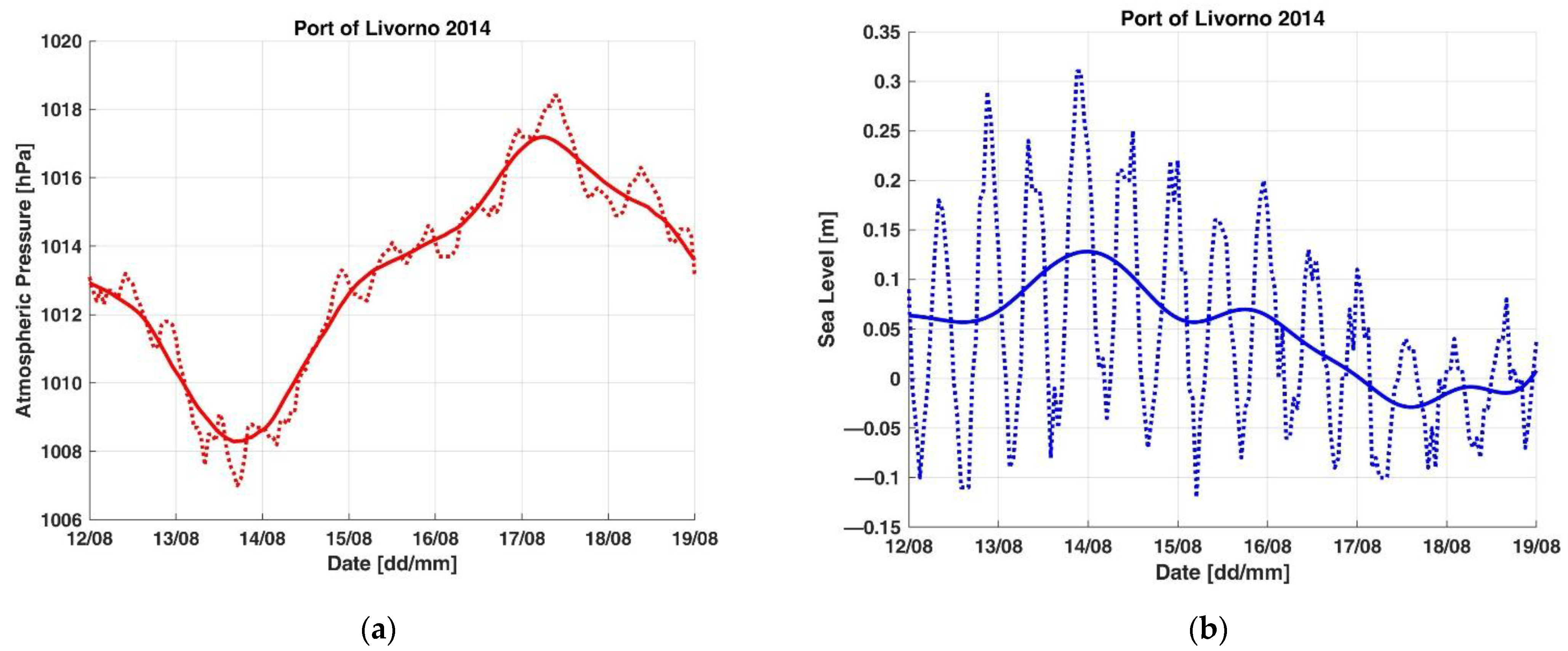
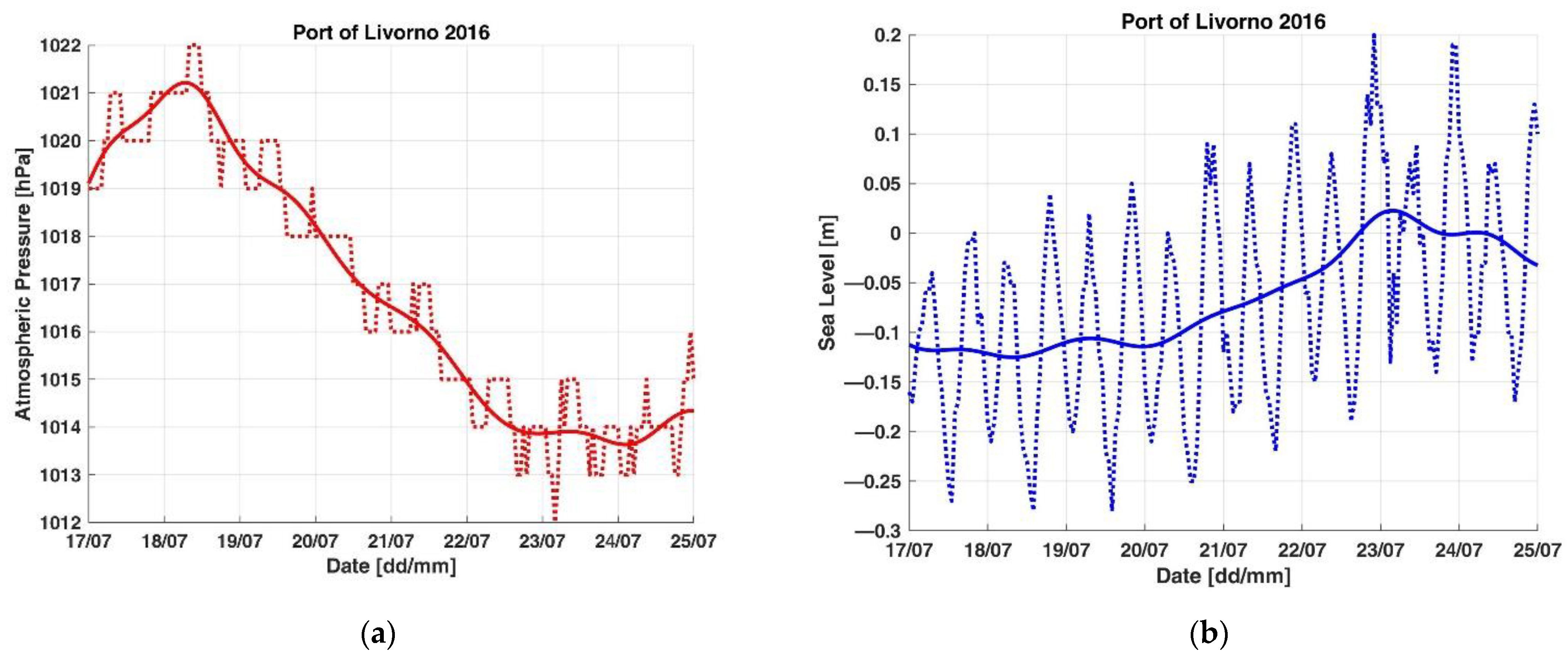
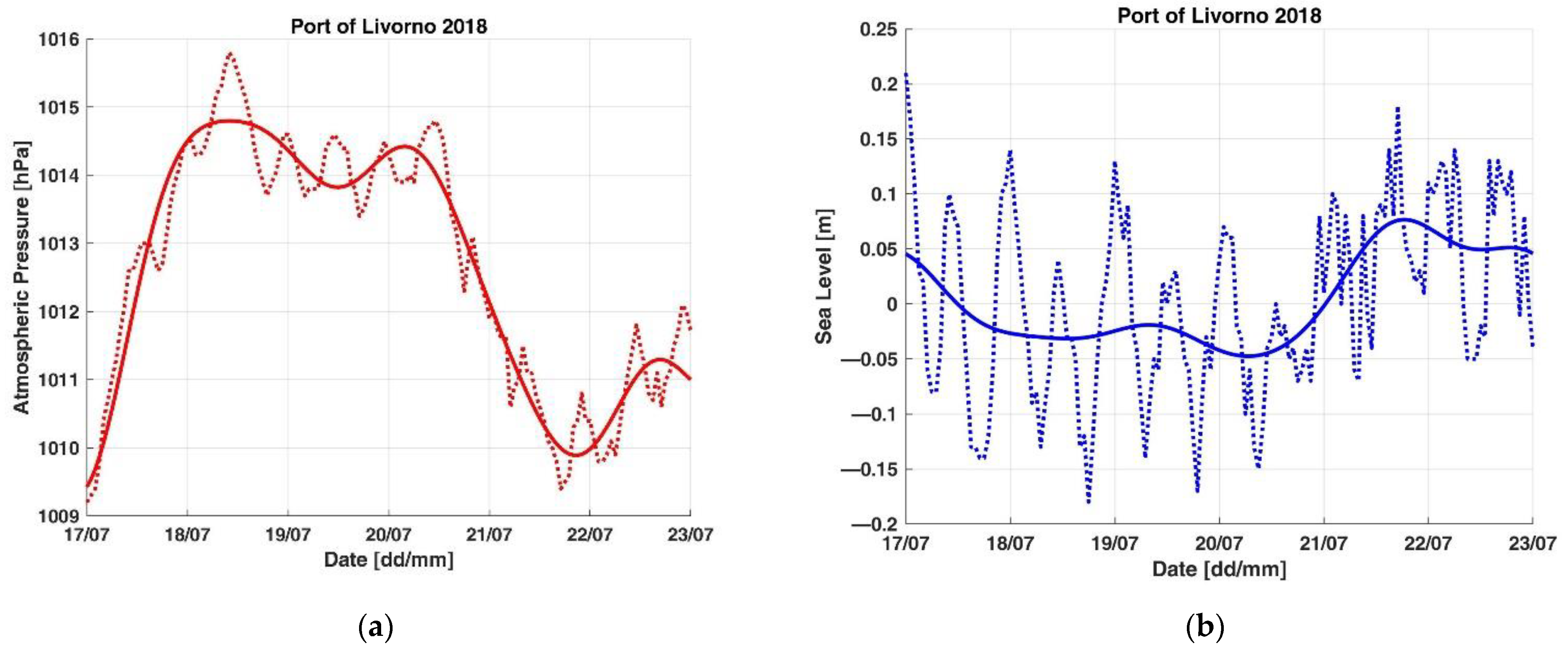
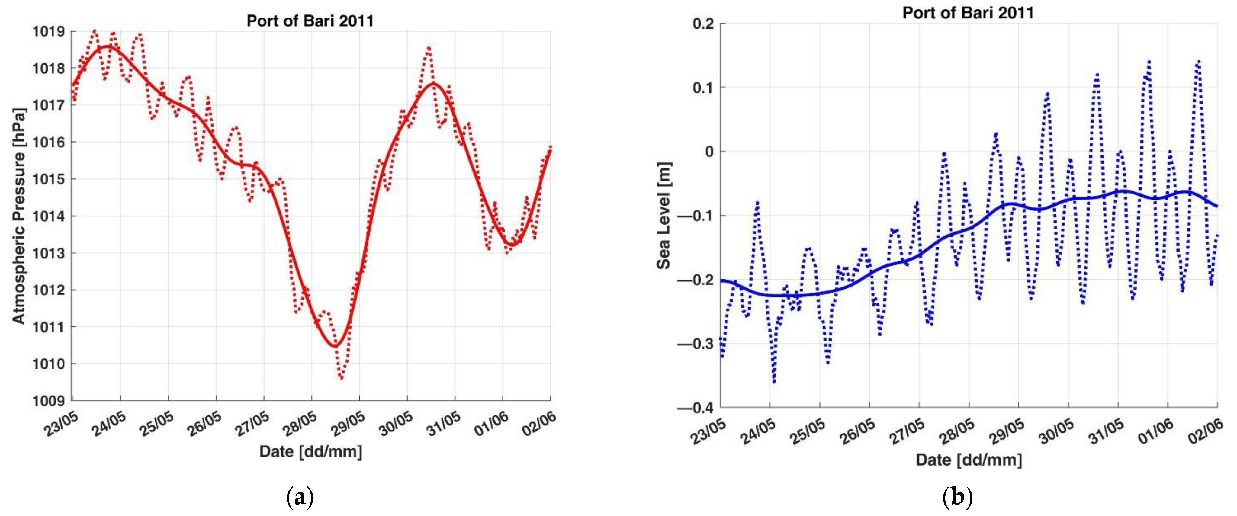
In Table 1 and Table 2 representative events that occurred since 2010 in Livorno and Bari harbours are listed, together with the estimates of Jph (data from 21 September 2015 to 24 March 2019 in Bari are not available). The plots of these events are shown in Appendix A, in Figure A1, Figure A2, Figure A3, Figure A4, Figure A5, Figure A6, Figure A7, Figure A8, Figure A9, Figure A10, Figure A11, Figure A12, Figure A13, Figure A14, Figure A15, Figure A16, Figure A17, Figure A18, Figure A19 and Figure A20 (except the events already shown in Figure 12 and Figure 13).
Starting from this statistic, the mean value (2 cm·hPa−1 for Livorno, 2.1 cm·hPa−1 for Bari) can be used as an estimate of Jph (which means to hypothesize a linear dependence of Δh from Δp).
Once known, the hydro-barometric transfer factor allows estimating for each basin a future change in sea level based on the measurement or forecasting of atmospheric pressure (it will be sufficient to multiply the variation of atmospheric pressure by the mean Jph factor and then reverse the sign, taking into account that pressure and level changes have opposite signs: when one increases, the other decreases).
By doing so, the average error on the forecasted meteorological tide (difference between the expected value and the measured one) is about 9.6% for Livorno and 8.2% for Bari, that is satisfactory for our purposes; otherwise, a better estimate could consider a non-linear variation of Δh as a function of Δp, at the cost of increased computational burden.
Once Jph has been evaluated, it is possible to estimate the forecasted sea level by means of a simple processing procedure that calculates the sum of two contributions: the astronomical tide (well-known, available from tide charts) and the meteorological one that, as seen, can be found as the product of the average hydrobarometric factor Jph (with the sign reversed) by the expected (or real-time acquired) atmospheric pressure gradient.
Therefore, the knowledge of Jph is very helpful in harbour waterside management: the effects of pressure variations on seawater depth can be applied to bathymetric maps in coastal areas: a change of atmospheric pressure can be converted, through Jph, into a forecasted meteorological tide and therefore in an expected sea level, and finally in a new bathymetric map.
Finally, it should be noted that it is appropriate to update continuously the estimate of Jph for a certain basin, in particular after events that change the topography (e.g., dredging operations, coastal erosion, sediment deposit, sea bottom subsidence). In any case, multi-decade statistics of Jph is needed if we want to evaluate the possible effect of long-term phenomena such as climate change on the hydrobarometric transfer factor.

3. Results

The system, even if it is still a prototype, was tested on some real events that occurred in Livorno and Bari harbours, achieving satisfactory results in signalling potentially dangerous conditions for a certain ship at a given instant.
In Figure 14a the center of the map of the port of Livorno is updated by means of data acquired on 24 February 2020 at 02:20; on the contrary, Figure 14b is referred to 5 December 2020 at 12:10; the user interface reports date, time and sea level of each measurement read from the archive. As we can see, sea level rises from −0.37 to 0.68 m; the consequent increase in sea level equal to 1.05 m causes an enlargement of the allowed area (in particular the green waterway in the middle of the map) and a reduction of the prohibited (red) one (the increase in sea level is partly due to astronomical tide and partly to a decrease in atmospheric pressure which changes approximately from 1023.9 to 994.8 hPa; pressure data at 24 February at 02:20 and on 5 December at 12:10 have been calculated by extrapolating the adjacent hourly measurements).
In Figure 15 the lower central area of Bari harbour is updated according to the values measured on 24 July 2020: in Figure 15a the map is at 17:30, while Figure 15b is referred at 23:30; the sea level is equal to 0.14 m in the first case, and it is to—0.38 m in the second case: then, there is a gradient of—0.52 m between the two different situations illustrated; this induces shrinkage of the allowed (green) area and an expansion of the prohibited (red) zone; atmospheric pressure rises from about 1007.4 to 1011.5 hPa within a few hours and then contributes to drop the sea level; in particular, we can see that the green waterway in the middle of the map becomes narrower, due to the decrease in the sea level.
Furthermore, the user interface shows coordinates and depth of the position pointed by the mouse at each instant; moreover, the traffic light shows by means of the correct colour if that position at the current time belongs to a forbidden, allowed or warning area: by keeping the mouse pointer in a certain position, it is possible to follow the evolution of its state over time.
In Figure 14, the bottom depth related to coordinates Easting 605,075, Northing 4,824,140 m pointed by the mouse arrow in the middle of the channel varies from 11.49 to 12.54 m, then the corresponding traffic light turns from red (prohibited position) to green (allowed position) colour (thresholds are fixed to 11.5 and 12.5 m). In the example in Figure 15, on the contrary, the depth of the position Easting 655,971, Northing 4,555,512 m in the middle of the map changes from 10.27 to 9.75 m, so its traffic light changes from green (permitted position) to yellow (warning position) light (higher threshold is equal to 10 m).
Therefore, the user interface implements the so-called virtual traffic lights (partition in red, yellow and green areas) customized for each vessel, depending on its draught: varying sea level, an area that initially was allowed (green), can become a warning (yellow) or forbidden area (red) for that ship, or vice versa; this application has been developed to support port communities (coast guards, port authorities, pilots, terminal operators) to plan and optimize coastal navigation (e.g., deciding when a ship can enter/leave a port or to choose its best route), ship moorings and docking performances (e.g., to which quay a vessel can access), logistics operations and ship loading (e.g., establishing the cargo of a vessel at the starting port according to the expected sea level at the destination), effectiveness in maritime works (e.g., dimensioning of breakwaters), and monitoring of water exchange in harbours; above all, it can be a helpful tool to port operators to increase port navigation safety, to prevent ship accidents, to manage emergencies such as ship stranding, or to reduce the risks of environmental damage (dispersion of pollutant) and economic impacts.
The system has been tried on several real cases by analyzing critical situations, providing satisfactory results in detecting hazardous areas; the examination of two accidents that occurred in the port of Livorno and Bari are described here.
As first, we describe the dynamic analysis of the bathymetry of the port of Livorno on 6 February 2021 (examination of an accident occurred in the past, so the bathymetry is updated by loading sea level values from a data storage): at 08:00 a container ship of 11.5 m draught stranded while was entering the port (the sea level measured by the hydrometer was 0.15 m). Figure 16a shows virtual traffic lights at the entrance area of the port at that time: threshold levels are selected at 11.5 and 12.5 m; the mouse pointer indicates the approximate location (Easting 604,380, Northing 4,822,105, m) where the vessel grounded; as we can see, the red virtual traffic light indicates that this position was forbidden for that ship at that moment because its updated depth (11.15 m) was smaller than the ship draught.
It is also worth noting that the position considered may not be forbidden for the same ship at another time (corresponding to different sea-level values, for example during a high tide), as well as the same position at the same time could be allowed for another vessel with smaller draught (which would result in different threshold levels).
For example, Figure 16b shows virtual traffic lights at the same position for the same ship on 10 February 2021 at 07:40: the greater sea-level value (0.55 m) makes the updated depth equal to 11.55 m, then a little greater than the ship draught, so that position belongs to a yellow or warning area. Note that the increase of 0.40 m in sea level between the two situations is partially due to a decrease of 14.6 hPa in atmospheric pressure.
As regards the port of Bari, on 12 July 2011 at about 10:00 a ship of 9 m draught struck the seabed at 8.45 m depth while approaching docks (the monitoring station was measuring: sea level −0.08 m); the dynamic analysis of the bathymetric map for this event had been executed: the updating of the map has been performed by reading from the archive sea level measurements related to that day. Figure 17a shows virtual traffic lights of a detail of the port at that time: thresholds are chosen equal to 9 and 10 m, respectively. As we can see, particular circumstances occur and a few red pixels (pointed by the mouse arrow) stand out in the middle of the green background (Easting 656,142, Northing 4,555,857 m). This is approximately the position where the ship collided with the anchoring systems of some mooring buoys (structures on the sea floor consisting of metal cages containing concrete inside); the peculiarity of this situation consists in the fact that the danger was concentrated in a very limited area inside a much wider area allowed (for that ship).
As we can see in Figure 17b at another time, for example, on 21 March 2012 at 08:00, during a low tide (sea level—0.59 m), the same position would be surrounded by a yellow area that that could make the danger better perceptible.
Overall, the usefulness of this application is the capability of detecting potentially dangerous areas in certain locations, at certain times, and, above all, for a given ship. In fact, the current state of virtual traffic lights depends on the position, on the specific moment, and on the threshold levels chosen; the last ones, in turn, depend on the draught of the ship taken into account.

4. Discussion and Conclusions

This article deals with the development of a system aimed at detecting and signaling potentially dangerous situations in coastal areas to decision makers (port authorities, coast guards, pilots), with the purpose of improving maritime safety by mitigating risk due to sea-level variations.
It is underlined the importance of monitoring, processing and forecasting environmental parameters in ports and gulfs. Here is a description of the results of observing and analysing activities in two test sites, Livorno and Bari harbours (Italy).
During tests performed by analyzing some real situations, the application correctly detected hazardous areas for a certain ship at a given instant, properly dividing the test area into allowed, warning and prohibited zones, with a spatial resolution equal to that with which multibeam surveys were performed.
The results achieved so far have been satisfactory to demonstrate the usefulness of the system: its use in the context of harbour waterside management can support port communities (port authorities, pilots) in analysing maritime accidents that occurred in the past as well as in planning and optimizing port activities and logistics operations, in particular:
  • in increasing effectiveness and safety of coastal maritime transport by choosing, for a given vessel and based on its draught, the best route to follow, or the most suitable pier to moor, or the best time when it can enter or leave a port (to avoid accidents such as stranding);
  • in optimizing cargo in the departure port (until a ship can be loaded based on the sea level forecasted at the port of arrival);
  • in planning the refloating of a ship (in case of accidents occurred), in order to mitigate the risk of environmental damages and economic losses for the community.
In particular, by using the forecasted astronomical tide and atmospheric pressure (converted into the expected meteorological tide through the use of the hydrobarometric transfer factor Jph), the dynamic bathymetric map allows improving the performances of port activities by planning them in advance.
In addition, the knowledge in advance of sea level in coastal areas may also be useful for:
  • optimizing the vessel docking (how to secure moorings to prevent tearing of ropes);
  • optimizing the effectiveness in maritime works (how to size breakwaters and docks based on the maximum sea level expected);
  • marine water quality control: assessing the concentration of pollutants (solute) on the basis of knowledge of the amount of seawater (solvent) at a certain moment.
In a hypothetical operational scenario, a local authority could manage a control room hosting a picture showing the dynamic bathymetric map of the harbour (virtual traffic lights), to receive useful support and take the best decisions, in order to ensure safety for people working or living in ports areas or gulfs; the same facility could also work on board ships, e.g., on PC or tablet.
Virtual traffic lights are obviously reliable on the assumption that the inputs of the system are, for instance, that the starting static bathymetric map can still represent the basin topography (otherwise it should be updated by performing new multibeam surveys), that multibeam surveys are performed with an appropriate resolution, that sea-level values acquired by a hydrometer working at a certain position are representative of the whole basin, and that forecasting of atmospheric parameters is accurate and known well in advance; under these conditions, tests performed in Livorno and Bari indicated an average error on the expected meteorological tide less than 10% that very rarely causes confusion about virtual traffic lights; in any case, increasing the number of mareographic stations in a basin, although it would increase installation costs, would allow a better spatial resolution in the dynamic updating of the bathymetric map, by using different sea-level values for each sub-domain into which the basin is divided.
Finally, the system is able to take into account other inputs such as wind effect and storm surges (not relevant and therefore neglected in this study), which are relevant especially in some locations and therefore should be provided as inputs to the sea level forecasting procedure to improve the effectiveness of the tool.

Author Contributions

Conceptualization, M.S. and O.F.; methodology, M.S. and O.F.; software, M.S. and O.F.; validation, M.S. and O.F.; formal analysis, M.S. and O.F.; investigation, M.S. and O.F.; resources, M.S. and O.F.; data curation, M.S.; writing—original draft preparation, M.S.; writing—review and editing, M.S. and O.F.; visualization, M.S. and O.F.; supervision, O.F.; project administration, M.S. and O.F.; funding acquisition, M.S. and O.F. All authors have read and agreed to the published version of the manuscript.

Funding

This research was funded within the framework of MENFOR Project (MEteo-tide Newtonian FORecasting) by several Italian Port Authorities, in particular Port Authority of Livorno (now named Port System Authority of the Northern Tyrrhenian Sea) and Port Authority of Bari (now called Port System Authority of the Southern Adriatic Sea) for the work described in this article.

Institutional Review Board Statement

Not applicable.

Informed Consent Statement

Not applicable.

Data Availability Statement

Meteo-mareographic data shown in this article, acquired by means of monitoring stations belonging to National Tidegauge Network managed by ISPRA, are available on the web site https://www.mareografico.it/ (accessed on 25 October 2021).

Computer Code Availability Statement

Not applicable.

Acknowledgments

The authors wish to thank Port Authorities of Livorno and Bari for providing bathymetric data and for their past financial support to the MENFOR Project within which these studies started (a special thanks to E. Pagnotta and M. Vivaldi who kindly provided us with a lot of useful information to carry out this work), Italian Coast Guard (in particular Cdr. Gennaro Fusco and Cdr. Stefano Carnevali) for the support to the research about port navigation safety, and D.A. Leoncini for his past contribution in the development of the software application. Part of this research was carried out when the first author was at OGS—National Institute of Oceanography and Applied Geophysics (Trieste, Italy). Finally, the authors thank the anonymous reviewers, whose comments and suggestions helped improve this work.

Conflicts of Interest

The authors declare no conflict of interest.

Appendix A

Figure A1. Low-frequency components of meteo-mareographic parameters acquired by ISPRA’s monitoring station in the port of Livorno from 7 to 16 September 2010: (a) atmospheric pressure; (b) sea level.
Applsci 11 10265 g0a1
Figure A2. Low-frequency components of meteo-mareographic parameters acquired by ISPRA’s monitoring station in the port of Livorno from 18 to 23 June 2011: (a) atmospheric pressure; (b) sea level.
Applsci 11 10265 g0a2
Figure A3. Low-frequency components of meteo-mareographic parameters acquired by ISPRA’s monitoring station in the port of Livorno from 13 to 20 July 2012 (a) atmospheric pressure; (b) sea level.
Applsci 11 10265 g0a3
Figure A4. Low-frequency components of meteo-mareographic parameters acquired by ISPRA’s monitoring station in the port of Livorno from 12 to 19 August 2014 (a) atmospheric pressure; (b) sea level.
Applsci 11 10265 g0a4
Figure A5. Low-frequency components of meteo-mareographic parameters acquired by ISPRA’s monitoring station in the port of Livorno from 6 to 15 June 2015: (a) atmospheric pressure; (b) sea level.
Applsci 11 10265 g0a5
Figure A6. Low-frequency components of meteo-mareographic parameters acquired by ISPRA’s monitoring station in the port of Livorno from 17 to 25 July 2016 (atmospheric pressure data have been acquired with resolution of 1 hPa): (a) atmospheric pressure; (b) sea level.
Applsci 11 10265 g0a6
Figure A7. Low-frequency components of meteo-mareographic parameters acquired by ISPRA’s monitoring station in the port of Livorno from 8 to 18 August 2017: (a) atmospheric pressure; (b) sea level.
Applsci 11 10265 g0a7
Figure A8. Low-frequency components of meteo-mareographic parameters acquired by ISPRA’s monitoring station in the port of Livorno from 17 to 23 July 2018: (a) atmospheric pressure; (b) sea level.
Applsci 11 10265 g0a8
Figure A9. Low-frequency components of meteo-mareographic parameters acquired by ISPRA’s monitoring station in the port of Livorno from 15 to 20 December 2018 (some missing sea level data on 18 December have been reconstructed by means of interpolation before low-pass filtering): (a) atmospheric pressure; (b) sea level.
Applsci 11 10265 g0a9
Figure A10. Low-frequency components of meteo-mareographic parameters acquired by ISPRA’s monitoring station in the port of Livorno from 20 to 26 May 2021: (a) atmospheric pressure; (b) sea level.
Applsci 11 10265 g0a10
Figure A11. Low-frequency components of meteo-mareographic parameters acquired by ISPRA’s monitoring station in the port of Bari from 30 August to 9 September 2010: (a) atmospheric pressure; (b) sea level.
Applsci 11 10265 g0a11
Figure A12. Low-frequency components of meteo-mareographic parameters acquired by ISPRA’s monitoring station in the port of Bari from 23 May to 2 June 2011: (a) atmospheric pressure; (b) sea level.
Applsci 11 10265 g0a12
Figure A13. Low-frequency components of meteo-mareographic parameters acquired by ISPRA’s monitoring station in the port of Bari from 21 November to 3 December 2011: (a) atmospheric pressure; (b) sea level.
Applsci 11 10265 g0a13
Figure A14. Low-frequency components of meteo-mareographic parameters acquired by ISPRA’s monitoring station in the port of Bari from 10 to 18 May 2012: (a) atmospheric pressure; (b) sea level.
Applsci 11 10265 g0a14
Figure A15. Low-frequency components of meteo-mareographic parameters acquired by ISPRA’s monitoring station in the port of Bari from 23 to 30 December 2012: (a) atmospheric pressure; (b) sea level.
Applsci 11 10265 g0a15
Figure A16. Low-frequency components of meteo-mareographic parameters acquired by ISPRA’s monitoring station in the port of Bari from 13 to 25 May 2014: (a) atmospheric pressure; (b) sea level.
Applsci 11 10265 g0a16
Figure A17. Low-frequency components of meteo-mareographic parameters acquired by ISPRA’s monitoring station in the port of Bari from 8 to 22 February 2015: (a) atmospheric pressure; (b) sea level.
Applsci 11 10265 g0a17
Figure A18. Low-frequency components of meteo-mareographic parameters acquired by ISPRA’s monitoring station in the port of Bari from 5 to 20 June 2015: (a) atmospheric pressure; (b) sea level.
Applsci 11 10265 g0a18
Figure A19. Low-frequency components of meteo-mareographic parameters acquired by ISPRA’s monitoring station in the port of Bari from 1 to 8 May 2019: (a) atmospheric pressure; (b) sea level.
Applsci 11 10265 g0a19
Figure A20. Low-frequency components of meteo-mareographic parameters acquired by ISPRA’s monitoring station in the port of Bari from 20 to 30 June 2020: (a) atmospheric pressure; (b) sea level.
Applsci 11 10265 g0a20

References

  1. Alyami, H.; Lee, P.T.-W.; Yang, Z.; Riahi, R.; Bonsall, S.; Wang, J. An advanced risk analysis approach for container port safety evaluation. Marit. Pol. Manag. 2014, 41, 634–650. [Google Scholar] [CrossRef]
  2. Bąk, A.; Zalewski, P. Determination of the Waterway Parameters as a Component of Safety Management System. Appl. Sci. 2021, 11, 4456. [Google Scholar] [CrossRef]
  3. Bartlett, D.; Celliers, L. (Eds.) Geoinformatics for Marine and Coastal Management, 1st ed.; CRC Press: Boca Raton, FL, USA, 2016. [Google Scholar] [CrossRef]
  4. Baylon, A.M.; Santos, E.M.R. Introducing GIS to TransNav and its Extensive Maritime Application: An Innovative Tool for Intelligent Decision Making? Trans. Nav. Int. J. Mar. Navig. Saf. Sea Transp. 2013, 7, 557–566. [Google Scholar] [CrossRef]
  5. Couper, A.D. Environmental port management. Marit. Pol. Manag. 1992, 19, 165–170. [Google Scholar] [CrossRef]
  6. Ducruet, C.; Berli, J.; Bunel, M. Geography versus topology in the evolution of the global container shipping network (1977–2016). In Geographies of Maritime Transport: Transport, Mobilities and Spatial Change; Wilmsmeier, G., Monios, J., Eds.; Edward Elgar Publishing: Cheltenham, UK, 2020; pp. 49–70. [Google Scholar] [CrossRef]
  7. Giuffrida, N.; Stojaković, M.; Twrdy, E.; Ignaccolo, M. The Importance of Environmental Factors in the Planning of Container Terminals: The Case Study of the Port of Augusta. Appl. Sci. 2021, 11, 2153. [Google Scholar] [CrossRef]
  8. Homsombat, W.; Yip, T.L.; Yang, H.; Fu, X. Regional cooperation and management of port pollution. Marit. Pol. Manag. 2013, 40, 451–466. [Google Scholar] [CrossRef]
  9. Hou, J. The temporal and spatial overview of global shipping routes. In Proceedings of the IEEE 23rd International Conference on Geoinformatics, Wuhan, China, 19–21 June 2015. [Google Scholar] [CrossRef]
  10. Lam, S.Y.-W.; Yip, T.L. The role of geomatics engineering in establishing the marine information system for maritime management. Marit. Pol. Manag. 2008, 35, 53–60. [Google Scholar] [CrossRef]
  11. Meyers, S.D.; Luther, M.E. The impact of sea level rise on maritime navigation within a large, channelized estuary. Marit. Pol. Manag. 2020, 47, 920–936. [Google Scholar] [CrossRef]
  12. Nguyen, T.-H.; Garrè, L.; Amdahl, J.; Leira, B.J. Benchmark study on the assessment of ship damage conditions during stranding. Ships Offshore Struct. 2012, 7, 197–213. [Google Scholar] [CrossRef]
  13. Nohheman, W. Benefits of dredging through reduced tidal waiting. Marit. Pol. Manag. 1981, 8, 17–20. [Google Scholar] [CrossRef]
  14. Ogura, T.; Inoue, T.; Uchihira, N. Prediction of Arrival Time of Vessels Considering Future Weather Conditions. Appl. Sci. 2021, 11, 4410. [Google Scholar] [CrossRef]
  15. Petraška, A.; Čižiūnienė, K.; Jarašūnienė, A.; Maruschak, P.; Prentkovskis, O. Algorithm for the assessment of heavyweight and oversize cargo transportation routes. J. Bus. Econ. Manag. 2017, 18, 1098–1114. [Google Scholar] [CrossRef] [Green Version]
  16. Titz, M.A. Port state control versus marine environmental pollution. Marit. Pol. Manag. 1989, 16, 189–211. [Google Scholar] [CrossRef]
  17. Vandermeulen, J.H. Environmental trends of ports and harbours: Implications for planning and management. Marit. Pol. Manag. 1996, 23, 55–66. [Google Scholar] [CrossRef]
  18. Vidmar, P.; Perkovič, M.; Gucma, L.; Łazuga, K. Risk Assessment of Moored and Passing Ships. Appl. Sci. 2020, 10, 6825. [Google Scholar] [CrossRef]
  19. Weintrit, A. Geoinformatics in Shipping and Marine Transport. In Challenge of Transport Telematics: TST 2016. Communications in Computer and Information Science; Mikulski, J., Ed.; Springer: Cham, Switzerland, 2016; Volume 640, pp. 13–25. [Google Scholar] [CrossRef]
  20. Yang, F.; Qiao, Y.; Wei, W.; Wang, X.; Wan, D.; Damaševičius, R.; Woźniak, M. DDTree: A Hybrid Deep Learning Model for Real-Time Waterway Depth Prediction and Smart Navigation. Appl. Sci. 2020, 10, 2770. [Google Scholar] [CrossRef] [Green Version]
  21. Istituto Idrografico della Marina. Tavole di Marea 2020; Istituto Idrografico della Marina: Genoa, Italy, 2019. [Google Scholar]
  22. Allen, J.S.; Denbo, D.W. Statistical Characteristics of the Large-Scale Response of Coastal Sea Level to Atmospheric Forcing. J. Phys. Oceanogr. 1984, 14, 1079–1094. [Google Scholar] [CrossRef]
  23. Crépon, M. Influence de la pression atmosphérique sur le niveau moyen de la Méditerranée Occidentale et sur le flux à travers le détroit de Gibraltar. Cah. Oceanogr. 1965, 1, 15–32. [Google Scholar]
  24. Faggioni, O. Measurement and Forecasting of Port Tide Hydrostatic Component in North Tyrrhenian Sea (Italy). Open J. Mar. Sci. 2020, 10, 52–77. [Google Scholar] [CrossRef]
  25. Faggioni, O.; Arena, G.; Bencivenga, M.; Bianco, G.; Bozzano, R.; Canepa, G.; Lusiani, P.; Nardone, G.; Piangiamore, G.L.; Soldani, M.; et al. The Newtonian approach in meteorological tide waves forecasting: Preliminary observations in the East Ligurian harbours. Ann. Geophys. 2006, 49, 1177–1187. [Google Scholar] [CrossRef]
  26. Faggioni, O.; Soldani, M.; Leoncini, D.A. Metrological Analysis of Geopotential Gravity Field for Harbor Waterside Management and Water Quality Control. Int. J. Geophys. 2013, 2013, 398956. [Google Scholar] [CrossRef]
  27. Garrett, C.; Majaess, F. Nonisostatic Response of Sea Level to Atmospheric Pressure in the Eastern Mediterranean. J. Phys. Oceanogr. 1984, 14, 656–665. [Google Scholar] [CrossRef] [Green Version]
  28. Le Traon, P.-Y.; Gauzelin, P. Response of the Mediterranean mean sea level to atmospheric pressure forcing. J. Geophys. Res. 1997, 102, 973–984. [Google Scholar] [CrossRef] [Green Version]
  29. Tsimplis, M.N. The Response of Sea Level to Atmospheric Forcing in the Mediterranean. J. Coast. Res. 1995, 11, 1309–1321. [Google Scholar]
  30. Tsimplis, M.N.; Vlahakis, G.N. Meteorological forcing and sea level variability in the Aegean Sea. J. Geophys. Res. 1994, 99, 9879–9890. [Google Scholar] [CrossRef]
  31. Faggioni, O.; Soldani, M.; Piangiamore, G.L.; Ferrante, A.; Bencivenga, M.; Arena, G.; Nardone, G. Harbour Water Management for port structures and sea bottom design, coast proximity navigation management, water quality control. In Proceedings of the 1st Mediterranean Days of Coastal and Port Engineering, Palermo, Italy, 7–9 October 2008. PIANC. [Google Scholar]
  32. Kanasewich, E.R. Time Sequence Analysis in Geophysics, 3rd ed.; The University of Alberta Press: Alberta, Canada, 1981. [Google Scholar]
  33. Krishnamurti, T.N. Numerical Weather Prediction. Annu. Rev. Fluid Mech. 1995, 27, 195–224. [Google Scholar] [CrossRef]
  34. Lynch, P. The Emergence of Numerical Weather Prediction: Richardson’s Dream; Cambridge University Press: Cambridge, UK, 2006. [Google Scholar]
  35. Lynch, P. The origins of computer weather prediction and climate modeling. J. Comp. Phys. 2008, 227, 3431–3444. [Google Scholar] [CrossRef] [Green Version]
  36. Stensrud, D.J. Parameterization Schemes: Keys to Understanding Numerical Weather Prediction Models; Cambridge University Press: Cambridge, UK, 2009. [Google Scholar]
  37. Telford, W.M.; Geldart, L.P.; Sheriff, R.E. Applied Geophysics, 2nd ed.; Cambridge University Press: Cambridge, UK, 1990. [Google Scholar] [CrossRef]
  38. Vilibić, I.; Dadic, V.; Ivanković, D.; Beg Paklar, G.; Čupić, S. Qualitative Analysis of Old and New Sea Level Measuring Techniques and Their Data Consistency. IEEE J. Ocean. Eng. 2007, 32, 428–435. [Google Scholar] [CrossRef]
  39. Palikaris, A.; Mavraeidopoulos, A.K. Electronic Navigational Charts: International Standards and Map Projections. J. Mar. Sci. Eng. 2020, 8, 248. [Google Scholar] [CrossRef] [Green Version]
  40. Bâki Iz, H. The effect of regional sea level atmospheric pressure on sea level variations at globally distributed tide gauge stations with long records. J. Geod. Sci. 2018, 8, 55–71. [Google Scholar] [CrossRef] [Green Version]
  41. Cabos, W.; de la Vara, A.; Álvarez-García, F.J.; Sánchez, E.; Sieck, K.; Pérez-Sanz, J.-I.; Limareva, N.; Sein, D.V. Impact of ocean-atmosphere coupling on regional climate: The Iberian Peninsula case. Clim. Dyn. 2020, 54, 4441–4467. [Google Scholar] [CrossRef]
  42. Chapman, S.; Lindzen, R.S. Atmospheric Tides: Thermal and Gravitational; Springer: Dordrecht, Holland, 1970. [Google Scholar] [CrossRef]
  43. Chelton, D.B.; Enfield, D.B. Ocean signals in tide gauge records. J. Geophys. Res. Solid Earth 1986, 91, 9081–9098. [Google Scholar] [CrossRef]
  44. Deser, C.; Tomas, R.A.; Sun, L. The Role of Ocean-Atmosphere Coupling in the Zonal-Mean Atmospheric Response to Arctic Sea Ice Loss. J. Clim. 2015, 28, 2168–2186. [Google Scholar] [CrossRef] [Green Version]
  45. Dickman, S.R. Theoretical investigation of the oceanic inverted barometer response. J. Geophys. Res. Solid Earth 1988, 93, 14941–14946. [Google Scholar] [CrossRef]
  46. Dobslaw, H.; Thomas, M. Atmospheric induced oceanic tides from ECMWF forecasts. Geophys. Res. Lett. 2005, 32, L10615. [Google Scholar] [CrossRef]
  47. Dong, D.; Gross, R.S.; Dickey, J.O. Seasonal variations of the Earth’s gravitational field: An analysis of atmospheric pressure, ocean tidal, surface water excitation. Geophys. Res. Lett. 1996, 23, 725–728. [Google Scholar] [CrossRef] [Green Version]
  48. El-Gindy, A.A.H.; Eid, F.M. Long-term variations of monthly mean sea level and its relation to atmospheric pressure in the Mediterranean Sea. Int. Hydrogr. Rev. 1990, 67, 147–159. [Google Scholar]
  49. Fu, L.-L.; Pihos, G. Determining the response of sea level to atmospheric pressure forcing using TOPEX/POSEIDON data. J. Geosphys. Res. 1994, 99, 24633–24642. [Google Scholar] [CrossRef]
  50. Garrett, C.; Toulany, B. Sea level variability due to meteorological forcing in the northeast Gulf of St. Lawrence. J. Geophys. Res. 1982, 87, 1968–1978. [Google Scholar] [CrossRef]
  51. Halliwell, G.R.; Allen, J.S. Large-Scale Sea Level Response to Atmospheric Forcing along the West Coast of North America, Summer 1973. J. Phys. Oceanogr. 1984, 14, 864–886. [Google Scholar] [CrossRef]
  52. Merriam, J.B. Atmospheric pressure and gravity. Geophys. J. Int. 1992, 109, 488–500. [Google Scholar] [CrossRef] [Green Version]
  53. Monserrat, S.; Ibbetson, A.; Thorpe, A.J. Atmospheric gravity waves and the ‘Rissaga’ phenomenon. Quart. J. R. Met. Soc. 1991, 117, 553–570. [Google Scholar] [CrossRef]
  54. Moon, I.-J. Impact of a coupled ocean wave-tide-circulation system on coastal modeling. Ocean Model 2005, 8, 203–236. [Google Scholar] [CrossRef]
  55. Ponte, R.M.; Gaspar, P. Regional analysis of the inverted barometer effect over the global ocean using TOPEX/POSEIDON data and model results. J. Geosphys. Res. 1999, 104, 15587–15601. [Google Scholar] [CrossRef]
  56. Spratt, R.S. Modelling the effect of atmospheric pressure variations on gravity. Geophys. J. Int. 1982, 71, 173–186. [Google Scholar] [CrossRef] [Green Version]
  57. Tai, C.-K. On the Quasigeostrophic Oceanic Response to Atmospheric Pressure Forcing: The Inverted Barometer Pumping; NOAA Technical Memorandum NOS OES 005; NOAA: Rockville, MA, USA, 1993. [Google Scholar]
  58. Trenberth, K.E. Seasonal variations in global sea level pressure and the total mass of the atmosphere. J. Geophys. Res. 1981, 86, 5238–5246. [Google Scholar] [CrossRef]
  59. Willebrand, J.; Philander, S.G.H.; Pacanowski, R.C. The Oceanic Response to Large-Scale Atmospheric Disturbances. J. Phys. Oceanogr. 1980, 10, 411–429. [Google Scholar] [CrossRef] [Green Version]
  60. Wills, R.C.J.; Armour, K.C.; Battisti, D.S.; Hartmann, D.L. Ocean-Atmosphere Dynamical Coupling Fundamental to the Atlantic Multidecadal Oscillation. J. Clim. 2019, 32, 251–272. [Google Scholar] [CrossRef]
  61. Wunsch, C. Bermuda sea level in relation to tides, weather, and baroclinic fluctuations. Rev. Geophys. Space Phys. 1972, 10, 1–49. [Google Scholar] [CrossRef]
  62. Wunsch, C.; Stammer, D. Atmospheric loading and the oceanic “inverted barometer” effect. Rev. Geophys. 1997, 35, 79–107. [Google Scholar] [CrossRef]
Figure 1. The test sites in Livorno and Bari harbours, in Italy (image from Google Earth).
Applsci 11 10265 g001
Figure 2. Bathymetric maps of test sites: (a) port of Livorno; (b) port of Bari; data have been provided by local Port Authorities.
Applsci 11 10265 g002aApplsci 11 10265 g002b
Figure 3. Virtual traffic lights in the port of Livorno: (a) thresholds equal to 10 and 11 m; (b) thresholds equal to 11.5 and 12.5 m.
Applsci 11 10265 g003
Figure 4. Virtual traffic lights in the port of Bari: (a) thresholds equal to 8 and 9 m; (b) thresholds equal to 9 and 10 m.
Applsci 11 10265 g004
Figure 5. Block diagram of bathymetry updating and virtual traffic lights.
Applsci 11 10265 g005
Figure 6. The ISPRA’s monitoring station in the port of Livorno: (a) the station (picture from https://www.mareografico.it/ (accessed on 25 October 2021)); (b) its position (10°17’57.62’’ E, 43°32’46.63’’ N, image from Google Earth).
Applsci 11 10265 g006
Figure 7. The ISPRA’s monitoring station in the port of Bari: (a) the station (picture from https://www.mareografico.it/ (accessed on 25 October 2021)); (b) its position (16°51′57.72” E, 41°08′24.74” N, image from Google Earth).
Applsci 11 10265 g007
Figure 8. Meteomareographic parameters acquired by ISPRA’s monitoring station in the port of Livorno from 27 November to 13 December 2019.
Applsci 11 10265 g008
Figure 9. Meteomareographic parameters acquired by ISPRA’s monitoring station in the port of Bari from 15 to 23 May 2011.
Applsci 11 10265 g009
Figure 10. Power spectral densities of meteomareographic parameters acquired by ISPRA’s monitoring station in the port of Livorno in 2019: (a) atmospheric pressure; (b) sea level; solid lines: lowfrequency components surviving the filtering; dashed lines: highfrequency components eliminated by the filtering.
Applsci 11 10265 g010
Figure 11. Power spectral densities of meteomareographic parameters acquired by ISPRA’s monitoring station in the port of Bari in 2011: (a) atmospheric pressure; (b) sea level; solid lines: lowfrequency components surviving the filtering; dashed lines: highfrequency components eliminated by the filtering.
Applsci 11 10265 g011
Figure 12. Low-frequency components of meteomareographic parameters acquired by ISPRA’s monitoring station in the port of Livorno from 27 November to 13 December 2019: (a) atmospheric pressure; (b) sea level; solid lines: low-frequency components surviving the filtering; dashed lines: high-frequency components eliminated by the filtering.
Applsci 11 10265 g012
Figure 13. Low-frequency components of meteo-mareographic parameters acquired by ISPRA’s monitoring station in the port of Bari from 15 to 23 May 2011: (a) atmospheric pressure; (b) sea level; solid lines: low-frequency components surviving the filtering; dashed lines: high-frequency components eliminated by the filtering.
Applsci 11 10265 g013
Figure 14. Detail of virtual traffic lights in the port of Livorno: (a) on 24 February 2020 at 02:20; (b) on 5 December 2020 at 12:10; thresholds equal to 11.5 and 12.5 m.
Applsci 11 10265 g014
Figure 15. Detail of virtual traffic lights in the port of Bari on 24 July 2020: (a) at 17:30; (b) at 23:30; thresholds equal to 9 and 10 m.
Applsci 11 10265 g015
Figure 16. Detail of virtual traffic lights in the port of Livorno: (a) on 6 February 2021 at 08:00; (b) on 10 February 2021 at 07:40; thresholds equal to 11.5 and 12.5 m.
Applsci 11 10265 g016aApplsci 11 10265 g016b
Figure 17. Detail of virtual traffic lights in the port of Bari: (a) on 12 July 2011 at 10:00; (b) on 21 March 2012 at 08:00; thresholds equal to 9 and 10 m.
Applsci 11 10265 g017
Table 1. Significant events occurred since 2010 in the port of Livorno.
StartEndΔp [hPa]Δh [cm]Jph [cm·hPa−1]
07/09/201016/09/201013.123.51.8
18/06/201123/06/20119.716.51.7
13/07/201220/07/201210.420.92
12/08/201419/08/20148.915.71.8
06/06/201515/06/2015918.92.1
17/07/201625/07/20167.614.81.9
08/08/201718/08/20177.916.12
17/07/201823/07/20184.912.42.5
15/12/201820/12/201814.123.31.7
27/11/201913/12/201919.545.22.3
20/05/202126/05/20217.4141.9
Table 2. Significant events occurred since 2010 in the port of Bari.
StartEndΔp [hPa]Δh [cm]Jph [cm·hPa−1]
30/08/201009/09/201010.919.31.8
15/05/201123/05/20118.116.82.1
23/05/201102/06/20118.116.32
21/11/201103/12/201111.121.72
10/05/201218/05/201214.9271.8
23/12/201230/12/20129.116.21.8
13/05/201425/05/201412.3292.4
08/02/201522/02/201525.255.52.2
05/06/201520/06/20151022.12.2
01/05/201908/05/201915.135.32.3
20/06/202030/06/202015.77.32.2
Publisher’s Note: MDPI stays neutral with regard to jurisdictional claims in published maps and institutional affiliations.

