
Downscaling Building Energy Consumption Carbon Emissions by Machine Learning
by
 , , , and
Zhuoqun Zhao
1,2, 
Xuchao Yang
3,
Han Yan
1,2,
Yiyi Huang
1,
Guoqin Zhang
1,4,
Tao Lin
1,4 and
Hong Ye
1,4,* 1
Key Lab of Urban Environment and Health, Institute of Urban Environment, Chinese Academy of Sciences, Xiamen 361021, China
2
University of Chinese Academy of Sciences, Beijing 100049, China
3
Ocean College, Zhejiang University, Zhoushan 316021, China
4
Xiamen Key Laboratory of Urban Metabolism, Xiamen 361021, China
*
Author to whom correspondence should be addressed.
Remote Sens. 2021, 13(21), 4346; https://doi.org/10.3390/rs13214346
Submission received: 26 August 2021
/
Revised: 21 October 2021
/
Accepted: 25 October 2021
/
Published: 28 October 2021
(This article belongs to the Special Issue Smart City Development and Remote Sensing Application in Urban Ecology)
Abstract
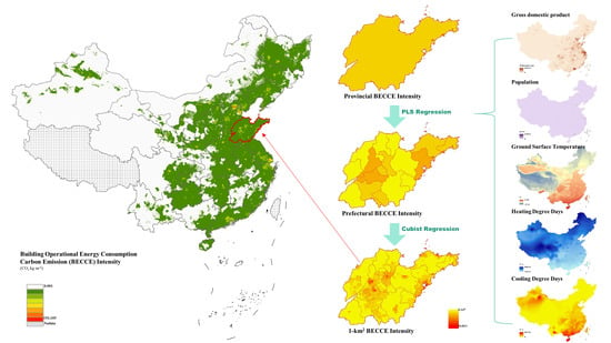
:The rapid rate of urbanization is causing increasing annual urban energy usage, drastic energy shortages, and pollution. Building operational energy consumption carbon emissions (BECCE) account for a substantial proportion of greenhouse gas emissions, crucially influencing global warming and the sustainability of urban socioeconomic development. As a foundation of building energy conservation, determination of refined statistics of BECCE is attracting increasing attention. However, reliable and accurate representation of BECCE remains lacking. This study proposed an innovative downscaling method to generate a gridded BECCE intensity benchmark dataset with 1 km2 spatial resolution. First, we calculated BECCE at the provincial level by energy balance table application. Second, on the basis of building climate demarcation, partial least squares regression models were used to establish the BECCE behavior equations for three climate regions. Third, Cubist regression models were built, retrieving down scale at the prefecture level to 1 km2 BECCE, which well-captured the complex relationships between BECCE and multisource covariates (i.e., gross domestic product, population, ground surface temperature, heating degree days, and cooling degree days). The downscaled product was verified using anthropogenic heat flux mapping at the same resolution. In comparison with other published pixel-based datasets of building energy usage, the gridded BECCE intensity map produced in this study showed good agreement and high spatial heterogeneity. This new BECCE intensity dataset could serve as a fundamental database for studies on building energy conservation and forecast carbon emissions, and could support decision makers in developing strategies for realizing the CO2 emission peak and carbon neutralization.
1. Introduction
With rapid development of urbanization globally, greenhouse gases associated with the urban metabolism continue to be emitted in huge quantities, substantially influencing global warming and sustainable urban socioeconomic development [1,2,3]. In 2018, building whole lifecycle energy usage emitted 9.7 Gt CO2, accounting for 39% of total energy-related CO2 emissions globally [4]. It is predicted that the current rapid rate of development will continue to drive energy consumption and carbon emissions even higher in the future, increasing even greater urgency to the need to address climate change [5]. In this context, some countries’ national greenhouse gas emission reduction targets have been proposed. For China, the targets aim to reach the CO2 emission peak by 2030 and achieve carbon neutralization by 2060, with the ultimate objective of achieving net-zero CO2 emissions.
Building operational energy consumption carbon emissions (BECCE) are responsible for over two-thirds of the total carbon emissions, and are expected to continue to rise as a result of the growing demand for building energy (Table A1) [6]. To explore the influential factors and to address the problems of energy usage and emission reduction in buildings, attention has increasingly focused on the calculation of BECCE at the fine scale [7].
Recent research has shown that a microclimate environment with a local impact on buildings is formed within a 1 km buffer zone of a building [8,9]. However, previous related studies focused primarily on building CO2 emissions within a regional macroclimate or mesoclimate background [10,11]. According to the widely used IPCC Guidelines for National Greenhouse Gas Inventories, BECCE is difficult to be measured directly and is closely dependent on the consumed energy when considering the carbon emission coefficients [12]. The main approaches used for BECCE estimation across the world can be generally grouped into two categories, ‘‘bottom-up” and ‘‘top-down” [13]. The bottom-up approach relies on thermodynamic-based software modeling and detailed energy samples of individual buildings, including engineering methods and sampling survey methods. Although accuratcy in BECCE estimation, the bottom-up approach has some significant limitations [14]. On one hand, the physical parameters or energy data with a high level of detail are unavailable to many complex organizations, limiting the accuracy and reliability of predicted BECCE. For example, the widely used building energy simulation tools (e.g., EnergyPlus [15,16], DOE-2 [17], ESP-r [18], system dynamics [19]) that utilize the engineering methods require precise building and environmental input parameters to achieve an accurate simulation, such as building construction characteristics, use patterns of equipment, and external or indoor temperatures, while the sampling survey methods require detailed survey data from energy bills of building samples [20]. On the other hand, these methods require tedious expert work and investigation, making them difficult to perform over large areas, and are cost-inefficient. Moreover, when extrapolating the estimated BECCE of building samples to represent the building stock based on the weights of sample representativeness, socioeconomic factors and human behaviors are often neglected.
The top-down approach, in contrast, regards the target building stock as an energy sink [19]. The classical top-down inventory-based method requires historical aggregated energy consumption data at different administrative units, which can be retrieved from some publicly available annual total bulk statistics, such as the residential and commercial building energy consumption surveys (RECS and CBECS) released by the US Energy Information Administration (EIA) [21], the annual report ‘Energy Consumption in the UK’ (ECUK) [22], China’s National Bureau of Statistics [23,24], and the International Energy Agency (IEA) database. Though it is useful in BECCE calculation, the classical inventory method is difficult to be applied in many study areas due to a lack of publicly available statistics. Some attempts have been made to address this problem, which built a multiple linear regression model between BECCE and the factors. For example, Liu et al. [25] established a linear relationship based on heating degree days and the change ratio of population to evaluate globally country-specific residential BECCE during the COVID-19 epidemic period. However, due to diverse demographic structures, socioeconomic patterns, and climatic conditions, the advanced artificial intelligence methods rather than linear regression models are more suitable for scientific estimation of BECCE, because they can explore complex nonlinear relations between BECCE and these variables, especially for large study areas. Recently, some machine learning algorithms such as Random Forest and Cubist models have been successfully applied to estimate population [26], electronic power consumption [27], and anthropogenic heat emission [28], which are relevant to BECCE estimation. Nevertheless, there are hardly any attempts at using those models with more BECCE-related ancillary data integrated to refine BECCE mapping.
Due to the current research status mentioned above, the approach for high-spatial-resolution BECCE estimation over large areas remains lacking. Such coarse data obtained by the aforementioned methods are short of spatial heterogeneity and lacking in details and accuracy over large areas, which hinder understanding of the relationship between BECCE and the urban environment, and restrict interdisciplinary studies using integrated environmental and social datasets in raster or gridded formats. Thus, development of an efficient approach for estimation of BECCE at the pixel level that could be easily integrated with other spatial data has become a new primary research interest of vital importance.
To address these gaps, this study attempts to propose a new machine learning-based downscaling approach to improve refined BECCE estimation. The flexible partial least squares (PLS) regression models and Cubist regression models were constructed to disaggregate statistical BECCE at different administrative levels into higher-resolution spatial units respectively, through capturing the relationships between varied ancillary geospatial layers and BECCE. In order to clearly demonstrate this novel approach, we generated an accurate gridded BECCE intensity benchmark dataset at 1 km2 spatial resolution over China in 2015. To the best of our knowledge, this study represents the first attempt to use a machine learning-based downscaling method that incorporates socioeconomic and geospatial data to estimate pixel-level BECCE. This new BECCE intensity dataset could serve as a fundamental database for studies on building energy conservation and forecast carbon emissions, and could support decision makers in developing strategies for realizing the CO2 emission peak and carbon neutralization.
2. Methodology
Accurate and reliable representation of fine-scale BECCE generally remains lacking; however, such information is in high demand for studies over large areas, especially in rapidly developing countries such as China. One feasible and practical approach to resolving this problem is to fuse downscaled data with fine-scale ancillary information, which is based on the idea of establishing relationships between a coarse-scale target variable and fine-scale auxiliary covariates [29,30,31]. Therefore, this study adopted a downscaling approach comprising four steps: (1) calculate provincial-level BECCE from different sources, (2) select predictors for BECCE mapping, (3) establish PLS regression models at the provincial level, and (4) build Cubist regression models at the prefecture level (Figure 1).
2.1. Calculating Provincial-Level BECCE from Different Sources
We first calculate provincial-level BECCE based on the IPCC Guidelines for National Greenhouse Gas Inventories. In mainland China, BECCE derive primarily from primary energy, heating power, and electric power [32]. In this study, we considered five energy types: coal (including raw coal, cleaned coal, other washed coal, briquettes, coke, and coke oven gas), petroleum products (including gasoline, diesel oil, and LPG), natural gas, heat, and electricity [33]. The composition of provincial-level BECCE can be formulated as follows:
where CFEN is the provincial BECCE, CFCOAL, CFPP, and CFNG are the CO2 emissions from provincial use of coal, petroleum products, and natural gas respectively, and CFHEAT and CFEL represent the CO2 emissions from provincial consumption of heat and electricity, respectively.
CEEN = CFCOAL + CFPP + CFNG +CFHEAT + CFEL
To facilitate calculation, all types of consumed energy were converted to standard coal equivalents. The total CO2 emissions from a certain energy type can be expressed as follows:
where Cei is the total provincial CO2 emissions from energy type i (i.e., coal, petroleum products, natural gas, heat, or electricity), Wej is the provincial final amount of consumption of energy type j based on the China Energy Statistical Yearbook, Gej is the conversion factor of energy type j consumption, which is the ratio of the final consumption of energy type j to standard coal consumption, Iej is the conversion factor of energy type j CO2 emissions, which is the amount of CO2 emissions per unit of standard coal consumption, and n is the total number of energy types (i = 1, 2, …, n) considered in this study.
2.2. Selection of Predictors for BECCE Mapping
In implementation of a downscaling method, to obtain a model with maximum predictability and effective transferability, it is necessary to screen variables guided by prior knowledge to evaluate their relevance and importance. Our previous study using factor analysis showed that building construction characteristics, socioeconomic environment, macroclimate conditions, and microclimate conditions have the greatest impact on BECCE in China [34,35]. Therefore, in this study, a suite of typical covariates was selected to represent these four factors in the PLS and Cubist regression models. Gridded population (POP) information, which was considered as the energy consumption membership to determine the CO2 emissions of a building in terms of lighting, cooking, heating, cooling, and ventilation, was used as the indicator of building characteristics [36,37]. Gross domestic product (GDP) was used to represent the socioeconomic environment [38,39]. Outdoor macroclimate conditions that substantially influence building energy usage can be represented by heating degree days (HDD18) and cooling degree days (CDD26), which were considered as indicators of the building energy consumption required for heating and cooling to maintain a comfortable indoor temperature [40]. The microclimate is generally defined as the local climate within 1 km2 of a building, which was represented by meteorological factors such as air humidity, solar radiation, and wind speed in some previous studies on building energy consumption [41,42]. In this study, we used the 0 cm ground surface temperature (GST) as the indicator of the microclimate environment.
2.3. Building Provincial-Level PLS Regression Models
PLS regression is a new multivariate statistical analysis model first proposed by Wold and Albano in 1983 [43]. It builds a linear regression model via data dimension reduction, information synthesis, and screening technology to extract new comprehensive components with optimal interpretation of the system [44]. The general underlying models of multivariate PLS regression can be expressed as follows:
where X is an n × m matrix of predictors, and Y is an n × p matrix of responses, T and U are n × l matrices that are projections of X and Y respectively, P and Q are m × l and p × l orthogonal loading matrices respectively, and E and F are matrices of the error terms, which are assumed to be independent and identically distributed random normal variables. Here, X and Y are decomposed to maximize the covariance between T and U.
X = TPT + E
Y = UQT + F
The PLS regression algorithm integrates the advantages of canonical correlation analysis, principal component analysis, and multiple linear regression analysis, making it applicable for a matrix of predictors that has more variables than observations and when multicollinearity exists among the independent variables [45]. In this study, provinces in China were initially divided into three groups on the basis of their regional characteristics (shown in the map of China in Figure 2, marked with different colors). Then, provincial-level PLS regression models were built for each group to capture the different associations between the various source variables and the target BECCE profile. The basis of the provincial grouping was China’s building climate demarcation (GB50176-93) (Ministry of Housing and Urban-Rural Development, 1993) [46], in which the energy-saving designs of buildings have notable differences. The groups comprised region I (northern part, most provinces in the Severe Cold Zone or Cold Zone), region II (central part, most provinces in the Hot Summer and Cold Winter Zone), and region III (southern part, most provinces in the Hot Summer and Warm Winter Zone or Mild Zone). Taking the above factor into consideration, for the covariates representing macroclimate conditions, HDD18 was selected as the indicator for region I, CDD26 was selected as the indicator for region III, and both HDD18 and CDD26 were selected as indicators for region II. We aggregated all the 1 km2 values of the predictors to the provincial level, and calculated the GDP per square kilometer, POP per square kilometer, average GST, average HDD18, and average CDD26, which were coordinated with calculated provincial-level BECCE intensity values (i.e., total BECCE of the province divided by provincial area). These PLS regression models representing the provincial-level relationships between BECCE intensity and related covariates were then applied to the corresponding covariates at the prefecture level to obtain primary estimates of prefectural-level BECCE intensity. The following step was to use the derived BECCE intensity estimations as the weighting layer for a standard dasymetric mapping approach to disaggregate the provincial-level BECCE to the final prefectural-level values [47,48].
2.4. Building Cubist Regression Models
Cubist regression, which was proposed based on the ideas of Quinlan [49,50], is a rule-based method applicable to multivariate linear regression. It operates by constructing intermediate linear models defined by sets of rules at each step of a model tree, then building a most suitable prediction based on the linear regression model at the terminal node of the tree, which is “smoothed” by taking the prediction from the former models into consideration, and subsequently, reducing the model tree to a set of rules via pruning and/or combined for simplification [51]. The general model of Cubist regression formed by two linear models can be expressed as follows:
where ζ(c) is the prediction from the current model, and ζ(p) is the prediction from the linear model in the previous node of the tree.
ζpar = (1—a) × ζ(p) + a × ζ(c)
As a deep-learning algorithm, the main advantages of the Cubist method are to add multiple training committee models to improve the predictive accuracy and to deal with nonlinear and complex multivariate relationships [52]. Simultaneously, it can be used to rank the relative importance of variables, which helps with model interpretation. Recently, the Cubist model has been proven to be a viable regression method and successfully used in various fields [53,54,55]. Thus, this study used Cubist regression models to generate gridded BECCE intensity estimates that were subsequently used for dasymetric disaggregation of prefectural-level BECCE data into gridded cells with 1 km2 spatial resolution, following the same principles as used in the downscaling approach of PLS regression fitting. This process has been applied successfully to Cubist-based dasymetric anthropogenic heat emission mapping by Chen et al. [28]. The Cubist models were implemented using the Cubist Package in the R environment.
3. Application and Verification
3.1. Data and Preprocessing
For clear demonstration of the proposed methodology, this study adopted mainland China as the study area (Figure 2). China is a country in East Asia, officially divided into 34 provincial administrative regions. In this study, Hong Kong, Macao, and Taiwan were excluded because their political and economic status differ from that of mainland China. Moreover, Tibet was not included because it does not have statistical data on energy consumption (these non-study areas are shown in the map of China in Figure 2, labeled “No data”). The BECCE data of 30 provinces used in the downscaling approach were collected from China’s Energy Statistical Yearbook for 2016 (http://www.stats.gov.cn/ accessed on 21 June 2017). The total final energy consumption needed for the BECCE calculation incorporated the items of wholesale and retail trade, hotels and restaurants, others, and residential consumption (urban and rural), extracted from the regional energy balance tables of this yearbook.
We used a series of socioeconomic, remote sensing, and geospatial datasets related to BECCE to build a set of covariates for fitting the PLS and Cubist regression models. Information regarding each covariate was extracted according to the corresponding grid at 1 km2 resolution using ArcGIS 10.7. The projection coordinates of all these grids were unified and their boundary data were completed to China’s borders through Kriging.
A number of ancillary variables were also included in the analysis. Gridded GDP and POP distribution maps for 2015 were acquired from the GDPGrid_China dataset and the PopulationGrid_China dataset for mainland China at 1 km2 spatial resolution respectively, published by the Data Center for Resources and Environmental Sciences of the Chinese Academy of Sciences (http://www.resdc.cn/ accessed on 11 December 2017). These two datasets were generated through building spatial correlation models with a map of land use and land cover change derived from Landsat TM imagery and other ancillary information. The resultant socioeconomic datasets have reasonably high accuracy at the county level.
The meteorological data used included GST, HDD18, and CDD26. Heating degree day and cooling degree day indices are frequently used indicators of the heating and cooling energy requirements of buildings. Daily HDD18 and CDD26 can be calculated using the basic formulas expressed in Equations (6) and (7), respectively [56]:
where T is the average air temperature of a day. Daily HDD18 and CDD26 can be accumulated over a year.
Raw meteorological data for 2015 were derived from daily GST and air temperature datasets provided by the China Meteorological Administration (http://data.cma.cn/ accessed on 4 August 2017). After processing to obtain the average GST of the entire year and the yearly accumulated HDD18 and CDD26 values of each meteorological station, the gridded GST map at 1 km2 resolution was constructed using ANUSPLIN software, with consideration of a digital elevation model, and the HDD18 and CDD26 maps were constructed through Kriging using ArcGIS.
3.2. Results
3.2.1. Spatial Distribution of the Five Covariates
The five covariates (i.e., GDP, POP, GST, HDD18, and CDD26) selected for the downscaling showed high spatial heterogeneity among cities, and exhibited notable differences in the three climate regions (Figure 3). For 2015, the GDP of a city ranged from 0.27 to 1859.00 billion yuan (average: 175.60 billion yuan). Among all the cities considered, Guangzhou, Suzhou, and Chengdu ranked as the top three. The POP of a city ranged from 8.38 × 10³ in Beitun (Xinjiang Province) to 15.23 × 10⁶ in Chengdu (Sichuan Province). The average value of POP was 3.62 × 10⁶. The GST varied from 0.66 °C in Yushu (Qinghai Province) to 30.23 °C in Sansha (Hainan Province), with an average value of 16.55 °C. Heating degree days ranged from 29.97 °C·day in Dongfang (Hainan Province) to 7149.65 °C·day in Da Hinggan Ling Prefecture (Heilongjiang Province), with an average value of 2270.96 °C·day. Cooling degree days ranged from 0.01 °C·day in Guoluo (Qinghai Province) to 609.93 °C·day in Dongfang (Hainan Province), with an average value of 116.12 °C·day. The average value of GST in regions I, II, and III was 8.98, 16.31, and 20.81 °C·day, respectively. The average value of heating degree days in region I was more than 2 and 5 times higher than that in regions II and III, respectively. The average value of cooling degree days in region III was nearly 3 and 2 times higher than that in regions I and II, respectively.
3.2.2. Energy Usage and Carbon Emissions at the Provincial Level from Energy-Balance Calculation
In 2015, the total amount of BECCE in China was 2060 Mt CO2, with an average value of 6.87 × 10⁷ tons of CO2 at the provincial level. Among the 30 provinces, Shandong, Hebei, and Heilongjiang provinces ranked as the top three with regard to BECCE, with values of 1.55 × 10⁸, 1.49 × 10⁸, and 1.48 × 10⁸ tons of CO2, respectively. The lowest value was 7.16 × 10⁶ tons of CO2 in Hainan Province (Figure 4). In terms of energy structure, the BECCE from electric power, heating power, and primary energy accounted for 43.48%, 27.68%, and 28.84% (raw coal accounting for 16.08%) respectively, of the total energy CO2 emissions. Emissions of CO2 from electricity represented the major proportion of BECCE, highlighting the need for ongoing work regarding the green low-carbon transformation in China (Figure 5a). The BECCE of residential buildings was 1.45 times higher than that of public buildings (Figure 5b).
3.2.3. Building PLS Regression Models for Provincial-Level BECCE
Table 1 lists the PLS regression models constructed for the three groups that have adjusted R2 values of 0.963, 0.961, and 0.804 for regions I, II, and III respectively, indicating that the basic models had sufficient explanatory power. On the basis of the regression analysis, we determined that all the relationships between BECCE intensity and the covariates in each region of China were positive. For region II, the importance of the effect of the covariates on BECCE in decreasing order was POP > GDP > HDD > CDD > GST. The order was similar for region III, except regarding consideration of HDD. High values of POP and GDP, e.g., as in central and southern China, directly reflect regional prosperity, which has a substantial impact on promoting BECCE. This finding is consistent with the result of Shi et al. [57], who found that GDP and population were important positive driving forces on BECCE at the prefecture level in China. For region I, HDD ranked as the covariate with the most important effect on BECCE, followed in decreasing order by GDP, POP, and GST. The macroclimate was the major factor regarding BECCE in the Severe Cold Zone and Cold Zone owing to the considerable building energy consumption required for heating to maintain a comfortable indoor temperature in winter. Therefore, HDD had the greatest impact on BECCE in region I, with a coefficient more than 2 and 8 times higher than that of GDP and POP, respectively. We also found that the controlling effect of the microclimate, represented by GST, made the smallest contribution to BECCE in all three regions. Nevertheless, according to our previous study, the microclimate around buildings should not be ignored [42]. This is because it can be improved reasonably easily for an investment level lower than that required for renovation of building characteristics or enhancement of socioeconomic conditions or the macroclimate.
The estimated prefectural-level BECCE is shown in Figure 6. The average value of prefectural-level BECCE was 5.11 × 10⁶ tons of CO2, and most cities had an intermediate value of BECCE (i.e., 1–8 × 10⁶ tons of CO2). The highest value of BECCE (4.96 × 10⁷ tons of CO2) was in Harbin, followed in decreasing order by Shenyang, Dalian, and Shijiazhuang. The value of BECCE of Kunyu (Xinjiang Province) was the lowest, i.e., 2.64 × 10⁴ tons of CO2. Generally, cities with high values of BECCE are located in provincial capitals with a prosperous economy and large population, and this is especially the case in northern China because of the need for heating in winter and the large volume of industry.
3.2.4. Pixel-Based Distribution of BECCE Intensity
Through joint use of multisource socioeconomic and environmental data in the Cubist regression downscaling approach, a gridded map of BECCE intensity for mainland China in 2015 was created with a spatial resolution of 1 km2 (Figure 7). The “Hu Huanyong Line”, which is a geographic demarcation line proposed by the famous geographer Hu Huanyong in 1935, that stretches from Heihe in northeastern China to Tengchong in southwestern China and shows the distinct spatial characteristics of the Chinese population, also marks a substantial difference in the BECCE intensity distribution across mainland China. The eastern side of the Hu Huanyong Line accounted for 88.81% of the BECCE of the entire study area, indicating the highly heterogeneous levels of urbanization and environmental pollution in China. Moreover, the pixel values of BECCE intensity varied considerably from 0.001 to 193.105 CO2 kg·m−2, with nearly 80% below the average value of 0.25 CO2 kg·m−2, showing the high level of heterogeneity. The pixels with high values of BECCE intensity were located mainly in major urban centers. Furthermore, high BECCE intensity was concentrated in urban areas of dynamically economic and prosperous regions such as Beijing, Tianjin, and Shanghai, with average BECCE intensity in the range of 16.49–57.12 CO2 kg·m−2 across downtown areas. In most cases, in comparison with peripheral cities, provincial capitals had higher BECCE intensity. However, built-up areas in some medium- or small-sized cities such as Shihezi (Xinjiang Province) had the highest average city value of BECCE intensity of up to 7.44 CO2 kg·m−2, probably attributable to extreme climate conditions in small spatial areas. For estimation of fine-scale BECCE intensity, GDP and POP, representing the socioeconomic conditions and energy consumption membership respectively, had the greatest influence (Figure 8). In comparison with the results of the PLS regression models, GST was shown to have a greater impact on BECCE intensity in region I at 1 km2 spatial resolution, which is consistent with the finding where there were differences on the importance of the driving factors on BECCE due to China’s different spatial classification [58], further indicating that its effect in the microenvironment should not be ignored in relation to building energy conservation.
3.2.5. Comparative Assessment of Accuracy
A per-pixel evaluation of the BECCE intensity maps was impossible owing to the lack of reference building energy consumption and BECCE data at the grid level (such information is scarce even at the prefecture level). Therefore, for a comparative assessment of accuracy, it is practical and reasonable to find other pixel-based data that are directly related to building energy usage. In this study, we compared the predicted BECCE intensity at the grid cell level with gridded anthropogenic heat flux (AHFb) that spatially represents the anthropogenic heat emission from buildings. Anthropogenic heat emission, which is the emission of anthropogenic waste heat into the urban land–atmosphere system driven by the energy consumption associated with human activities, plays an important role in urban climate and environment studies. Previous related studies have shown that anthropogenic heat emissions arise from industrial processing, heating and cooling of buildings, vehicle exhausts, and human metabolism [59,60]. Although there is high demand for reliable and accurate representation of anthropogenic heat emission across China, it is difficult to estimate at the regional scale because of limited data. Recently, Chen et al. [28] published a gridded AHFb benchmark dataset at 1 km2 spatial resolution for China in 2010 using the same principle of the Cubist-based downscaling approach with fusion off points-of-interest data of buildings and multisource remote sensing data. Based on the above, Pearson correlation analysis was conducted to explore the relationship between the estimated BECCE intensity and AHFb, which were processed to the same pixel position, normalized, and finally extracted using a 1 km2 fishnet.
Table 2 shows the results of the Pearson correlation analysis of the predicted BECCE intensity and the AHFb for the entire study area, region I, region II, and region III. For the entire study area, BECCE intensity was correlated positively with AHFb (R = 0.620, p = 0.01), and the strength of the correlation in region I was higher than that in regions II and III.
4. Discussion
4.1. Advantages of the Method
Downscaling approaches have been commonly applied to create accurate spatially explicit products in various fields (e.g., gridded population, GDP, electronic power consumption). In this study, crucially important elements were selected. PLS was applied for constructing BECCE driving mechanism behavior equations because it could effectively offset the collinear contribution among driving factors. Meanwhile, the Cubist algorithm proved its advantage for fine-scale data training and was used to refine our result. Comparing with Random Forest regression models, BECCE intensity data in urban centers of some large metropolitan areas retrieved by Cubist regression models was within the range of 16.49–57.12 CO2 kg·m−2, which is more scientific than the 0.002–7.438 CO2 kg·m−2 retrieved by the Random Forest method.
4.2. Comparison of Normalized BECCE Intensity and AHFb for Eight Metropolitan Cities in China
As a further demonstration of the relationship between BECCE intensity and AHFb, and to provide another form of accuracy assessment, Figure 9 shows the predicted BECCE intensity and AHFb in eight metropolitan cities: Beijing, Shanghai, Guangzhou, Wuhan, Xiamen, Chengdu, Harbin, and Urmqi. Owing to the different times of data collection, the analysis focuses on the relative change of values in different regions of the cities. In comparing BECCE intensity with AHFb, we found two types of spatial pattern highly replicated in all eight cities. First, areas with high BECCE intensity were distributed mainly in central cities, which generally have high values of AHFb. Second, high BECCE intensity and AHFb occurred mainly in dense residential and commercial areas in urban centers, exhibiting the characteristic of agglomeration. For example, evident high BECCE intensity was found in the Dongcheng and Xicheng districts of Beijing and the Jingan and Huangpu districts of Shanghai, which are well-developed urban areas with high-density buildings and prosperous businesses. These results showed that the proposed methodology is effective in capturing the main spatial characteristics of BECCE intensity and producing a reasonable spatial distribution of BECCE intensity. The findings demonstrated that BECCE intensity has a close relationship with AHFb in China, and that the method of estimation of BECCE intensity is reliable and accurate.
4.3. Limitations
The downscaling approaches suffer from an inherent limitation that they lack consideration of the variation of the statistical data on the same type of parcel due to time lag. At the same time, each of these input ancillary geospatial layers introduces its own uncertainty because of its inherent errors in location or in attribution. Perhaps most important, however, is that significant uncertainties arise from the difficulties in attempting to quantify and assess the link between the pixel-level BECCE and the ancillary layers, as the relations are typically uncertain and sensitive to local contextual factors, such as human behaviors, environmental consciousness, local fuel and electricity prices, air temperature change, and the vagaries of random chance. In addition, the BECCE distribution under different land form and land use patterns varies from urban core areas to suburban or rural areas, which has not been taken into consideration in this study.
5. Conclusions
In the context of rapid urbanization globally, urban energy consumption is rising annually. The continuous growth of BECCE restricts urban sustainable development, resulting in increasing energy shortages and energy-related pollution. As a foundation of building energy conservation, the determination of refined statistics of BECCE is attracting increasing attention. This study produced an innovative updated and comprehensive perspective of BECCE to satisfy the growing demand for a national database of BECCE profiles and to fill certain knowledge gaps. Based on the principle of downscaling, we proposed a novel method for gridded BECCE mapping that integrates socioeconomic and remote sensing data in flexible PLS and Cubist regression models, which were constructed to capture the complex relationships between covariates (i.e., GDP, POP, GST, HDD18, and CDD26) and BECCE intensity at the provincial and prefecture levels, respectively. We successfully generated a reasonable and accurate dataset of the estimated pixel-based BECCE intensity for China, which is closely related to human activities, with 1 km2 spatial resolution.
The newly developed gridded BECCE intensity dataset with high spatial heterogeneity could serve as a fundamental database for further studies on building energy conservation. The established dataset could also be used to further explore the relationships between BECCE intensity and socioeconomic factors and the urban environment, which would contribute to improved sustainable urban development. Moreover, the developed modeling technique could be applied to forecasting carbon emissions and studies on the CO2 emission peak and carbon neutralization. In this study, there is no distinction between different land use and land cover change in their downscaling approach. In the future, a more refined study area (the urban built-up land) will be focused on to estimate the downscaling-based BECCE distribution in the urban land use area, and to further explore the relationship with the BECCE distribution and urban three-dimensional buildings [61,62].
Author Contributions
Conceptualization, Z.Z. and H.Y. (Hong Ye); methodology, Z.Z. and H.Y. (Hong Ye); software, X.Y. and Y.H.; validation, X.Y.; formal analysis, Z.Z.; investigation, Z.Z.; resources, H.Y. (Han Yan); data curation, H.Y. (Hong Ye); writing—original draft preparation, Z.Z.; writing—review and editing, Z.Z. and H.Y. (Hong Ye); visualization, Z.Z.; supervision, G.Z.; project administration, T.L.; funding acquisition, H.Y. (Hong Ye) and T.L. All authors have read and agreed to the published version of the manuscript.
Funding
National Natural Science Foundation of China, grant numbers 41771570, 41971019, 41771573, and 41871167. The International Partnership Program of Chinese Academy of Sciences, grant number 132c35kysb2020007.
Institutional Review Board Statement
Not applicable.
Informed Consent Statement
Not applicable.
Data Availability Statement
The data presented in this study are available upon request from the corresponding author.
Acknowledgments
We thank the Data Center for Resources and Environmental Sciences of the Chinese Academy of Sciences (http://www.resdc.cn/ accessed on 11 December 2017) for providing gridded GDP and population datasets free of charge. We are also grateful to the reviewers for their helpful comments and suggestions for improving the manuscript.
Conflicts of Interest
The authors declare no conflict of interest.
Appendix A

Table A1.
Abbreviations in this paper.
| Abbreviation | Definition | Abbreviation | Definition |
|---|---|---|---|
| BECCE | Building operational energy consumption carbon emissions | BECCEI | building operational energy consumption carbon emission intensity |
| UN | United Nations | AHFb | anthropogenic heat flux |
| SDGs | Sustainable Developments Goals | POP | population |
| RECS | Residential Energy Consumption Surveys | GDP | gross domestic product |
| CBECS | Commercial Buildings Energy Consumption Surveys | HDD18 | heating degree days |
| EIA | Energy Information Administration | CDD26 | cooling degree days |
| ECUK | Energy Consumption in the UK | GST | ground surface temperature |
| PLS | partial least squares regression |
References
- Liu, Y.; Wang, M.; Feng, C. Inequalities of China’s regional low-carbon development. J. Environ. Manag. 2020, 274, 1–11. [Google Scholar] [CrossRef]
- Zhang, Y.; Zhao, L.; Zhang, H.; Tan, T. The impact of economic growth, industrial structure and urbanization on carbon emission intensity in China. Nat. Hazards 2014, 73, 579–595. [Google Scholar] [CrossRef]
- Flückiger, M.; Ludwig, M. Geography, human capital and urbanization: A regional analysis. Econ. Lett. 2018, 168, 10–14. [Google Scholar] [CrossRef] [Green Version]
- Energy Information Administration. 2019 Global Status Report for Buildings and Construction; United Nations Environment Programme: Washington, DC, USA, 2019. [Google Scholar]
- Ramaswami, A.; Tong, K.; Canadell, J.; Jackson, R.; Stokes, E.; Dhakal, S.; Finch, M.; Jittrapirom, P.; Singh, N.; Yamagata, Y.; et al. Carbon analytics for net-zero emissions sustainable cities. Nat. Sustain. 2021, 4, 460–463. [Google Scholar] [CrossRef]
- Energy Information Administration. GlobalABC Roadmap for Buildings and Construction 2020–2050; Federal Ministry of Economic Affairs and Energy: Washington, DC, USA, 2020.
- Sztubecka, M.; Skiba, M.; Mrówczyńska, M.; Bazan-Krzywoszańska, A. An innovative decision support system to improve the energy efficiency of buildings in urban areas. Remote Sens. 2020, 12, 259. [Google Scholar] [CrossRef] [Green Version]
- Yang, X.; Zhao, L. Impacts of urban microclimate on building energy performance: A review of research methods. Build. Sci. 2015, 31, 1–7. [Google Scholar]
- Shahrestani, M.; Yao, R.; Luo, Z.; Turkbeyler, E.; Davies, H. A field study of urban microclimates in London. Renew. Energy 2015, 73, 3–9. [Google Scholar] [CrossRef] [Green Version]
- Li, J.; Colombier, M. Managing carbon emissions in China through building energy efficiency. J. Environ. Manag. 2009, 90, 2436–2447. [Google Scholar] [CrossRef]
- Kahn, M.; Kok, N.; Quigley, J. Carbon emissions from the commercial building sector: The role of climate, quality, and incentives. J. Publ. Econ. 2014, 113, 1–12. [Google Scholar] [CrossRef]
- Eggleston, H.; Buendia, L.; Miwa, K.; Ngara, T.; Tanabe, K. 2006 IPCC Guidelines for National Greenhouse gas Inventories; IPCC National Greenhouse Gas Inventories Programme: Washington, DC, USA, 2006; pp. 1–20. [Google Scholar]
- Kadir, A.; Nora, M. A review of data-driven building energy consumption prediction studies. Renew. Sustain. Energy Rev. 2018, 81, 1192–1205. [Google Scholar]
- Zhao, H.; Magoules, F. A review on the prediction of building energy consumption. Renew. Sustain. Energy Rev. 2012, 16, 3586–3592. [Google Scholar] [CrossRef]
- Yang, X.; Peng, L.L.H.; Jiang, Z.; Chen, Y.; Yao, L.; He, Y.; Xu, T. Impact of urban heat island on energy demand in buildings: Local climate zones in Nanjing. Appl. Energy 2020, 260, 1–13. [Google Scholar] [CrossRef]
- Fumo, N.; Mago, P.; Luck, R. Methodology to estimate building energy consumption using EnergyPlus Benchmark Models. Energy Build. 2010, 42, 2331–2337. [Google Scholar] [CrossRef]
- Xu, P.; Huang, Y.J.; Miller, N.; Schlegel, N.; Shen, P. Impacts of climate change on building heating and cooling energy patterns in California. Energy 2012, 44, 792–804. [Google Scholar] [CrossRef]
- Strachan, P.; Kokogiannakis, G.; Macdonald, I. History and development of validation with the ESP-r simulation program. Build. Environ. 2008, 43, 601–609. [Google Scholar] [CrossRef] [Green Version]
- Zhou, W.; Moncaster, A.; Reiner, D.M.; Guthrie, P. Developing a generic System Dynamics model for building stock transformation towards energy efficiency and low-carbon development. Energy Build. 2020, 224, 1–17. [Google Scholar] [CrossRef]
- Ye, H.; Pan, L.; Chen, F.; Wang, K.; Huang, S. Direct carbon emission from urban residential energy consumption: A case study of Xiamen, China. Acta Ecol. Sin. 2010, 30, 3802–3811. [Google Scholar]
- EIA. 2018 Commercial Buildings Energy Consumption Survey; U.S. Department of Energy: Washington, DC, USA, 2021.
- Department for Business, Energy& Industrial Strategy. Energy Consumption in the UK (ECUK) 1970 to 2020. Available online: https://assets.publishing.service.gov.uk/government/uploads/system/uploads/attachment_data/file/1021836/Energy_Consumption_in_the_UK_2021.pdf (accessed on 30 September 2021).
- Huo, T.; Ma, Y.; Yu, T.; Cai, W.; Liu, B.; Ren, H. Decoupling and decomposition analysis of residential building carbon emissions from residential income: Evidence from the provincial level in China. Environ. Impact Assess. Rev. 2021, 86, 1–12. [Google Scholar] [CrossRef]
- Li, D.; Huang, G.; Zhang, G.; Wang, J. Driving factors of total carbon emissions from the construction industry in Jiangsu Province, China. J. Cleaner Prod. 2020, 276, 1–14. [Google Scholar] [CrossRef]
- Liu, Z. Near-real-time monitoring of global CO2 emissions reveals the effects of the COVID-19 pandemic. Nat. Commun. 2020, 11, 1–12. [Google Scholar] [CrossRef] [PubMed]
- Stevens, F.; Gaughan, A.; Linard, C.; Tatem, A. Disaggregating census data for population mapping using Random Forests with remotely-sensed and ancillary data. PLoS ONE 2015, 10, e0107042. [Google Scholar] [CrossRef] [PubMed] [Green Version]
- Jin, C.; Zhang, X.; Yang, X.; Zhao, N.; Ouyang, Z.; Yue, W. Mapping China’s electronic power consumption using points of interest and remote sensing data. Remote Sens. 2021, 13, 1058. [Google Scholar] [CrossRef]
- Chen, Q.; Yang, X.; Ouyang, Z.; Zhao, N.; Jiang, Q.; Ye, T.; Qi, J.; Yue, W. Estimation of anthropogenic heat emissions in China using Cubist with points-of-interest and multisource remote sensing data. Environ. Pollut. 2020, 266, 1–10. [Google Scholar] [CrossRef] [PubMed]
- Ge, Y.; Jin, Y.; Stein, A.; Yuehong, C.; Wang, J.; Wang, J.; Cheng, Q.; Bai, H.; Liu, M.; Atkinson, P.M. Principles and methods of scaling geospatial Earth science data. Earth-Sci. Rev. 2019, 197, 1–17. [Google Scholar] [CrossRef]
- Liao, Y.; Wang, J.; Meng, B.; Li, X. A method of spatialization of statistical population. Acta Geogr. Sin. 2007, 62, 1110–1119. [Google Scholar]
- Liao, Y.; Li, D.; Zhang, N. Comparison of interpolation models for estimating heavy metals in soils under various spatial characteristics and sampling methods. Trans. GIS 2018, 22, 409–434. [Google Scholar] [CrossRef]
- Department of Energy Statistics, National Bureau of Statistics, People’s Republic of China. China Energy Statistical Yearbook 2016; China Statistics Press: Beijing, China, 2016. [Google Scholar]
- Li, W.; Zhou, Y.; Cetin, K.; Eom, J.; Wang, Y.; Chen, G.; Zhang, X. Modeling urban building energy use: A review of modeling approaches and procedures. Energy 2017, 141, 2445–2457. [Google Scholar] [CrossRef]
- Ye, H.; Ren, Q.; Shi, L.; Song, J.; Hu, X.; Li, X.; Zhang, G.; Lin, T.; Xue, X. The role of climate, construction quality, microclimate, and socio-economic conditions on carbon emissions from office buildings in China. J. Clean. Prod. 2018, 171, 911–916. [Google Scholar] [CrossRef]
- Ye, H.; Qiu, Q.; Zhang, G.; Lin, T.; Li, X. Effects of natural environment on urban household energy usage carbon emissions. Energy Build. 2013, 65, 113–118. [Google Scholar] [CrossRef]
- Timmons, D.; Zirogiannis, N.; Lutz, M. Location matters: Population density and carbon emissions from residential building energy use in the United States. Energy Res. Soc. Sci. 2016, 22, 137–146. [Google Scholar] [CrossRef]
- Ye, H.; Wang, K.; Zhao, X.; Chen, F.; Li, X.; Pan, L. Relationship between construction characteristics and carbon emissions from urban household operational energy usage. Energy Build. 2011, 43, 147–152. [Google Scholar] [CrossRef]
- Delmastro, C.; Mutani, G.; Schranz, L.; Vicentini, G. The role of urban form and socio-economic variables for estimating the building energy savings potential at the urban scale. Int. J. Heat Technol. 2015, 33, 91–100. [Google Scholar] [CrossRef]
- Shi, K.; Yu, B.; Zhou, Y.; Chen, Y.; Yang, C.; Chen, Z.; Wu, J. Spatiotemporal variations of CO2 emissions and their impact factors in China: A comparative analysis between the provincial and prefectural levels. Appl. Energy 2019, 233-234, 170–181. [Google Scholar] [CrossRef]
- Yang, L.; Yan, H.; Lam, J.C. Thermal comfort and building energy consumption implications—A review. Appl. Energy 2014, 115, 164–173. [Google Scholar] [CrossRef]
- Skelhorn, C. A Fine Scale Assessment of Urban Greenspace Impacts on Microclimate and Building Energy in Manchester. Ph.D. Thesis, The University of Manchester, Manchester, UK, 2013. [Google Scholar]
- Ye, H.; Hu, X.; Ren, Q.; Lin, T.; Li, X.; Zhang, G.; Shi, L. Effect of urban micro-climatic regulation ability on public building energy usage carbon emission. Energy Build. 2017, 2017, 553–559. [Google Scholar] [CrossRef]
- Wold, S.; Sjostrom, M.; Eriksson, L. PLS-regression: A basic tool of chemometrics. Chemom. Intell. Lab. Syst. 2001, 58, 109–130. [Google Scholar] [CrossRef]
- Geladi, P.; Kowalski, B.R. Partial least-squares regression: A tutorial. Anal. Chim. Acta 1986, 185, 1–17. [Google Scholar] [CrossRef]
- Carrascal, L.M.; Galvan, I.; Gordo, O. Partial least squares regression as an alternative to current regression methods used in ecology. Oikos 2009, 118, 681–690. [Google Scholar] [CrossRef]
- Wan, K.K.W.; Li, D.H.W.; Yang, L.; Lam, J.C. Climate classifications and building energy use implications in China. Energy Build. 2010, 42, 1463–1471. [Google Scholar] [CrossRef]
- Nagle, N.N.; Buttenfield, B.P.; Leyk, S.; Speilman, S. Dasymetric modeling and uncertainty. Ann. Assoc. Am. Geogr. 2014, 104, 80–95. [Google Scholar] [CrossRef] [Green Version]
- Jia, P.; Gaughan, A.E. Dasymetric modeling: A hybrid approach using land cover and tax parcel data for mapping population in Alachua County, Florida. Appl. Geogr. 2016, 66, 100–108. [Google Scholar] [CrossRef]
- Quinlan, J.R. Learning with Continuous Classes, 1. In Proceedings of the 5th Australian Joint Conference on Artificial Intelligence, Hobart, Tasmania, 16–18 November 1992; pp. 343–348. [Google Scholar]
- Quinlan, J.R. Combining instance-based and model-based learning, 1. In Proceedings of the Tenth International Conference on Machine Learning, Amherst, MA, USA, 27–29 June 1993; pp. 236–243. [Google Scholar]
- Kuhn, M.; Johnson, K. Applied Predictive Modeling; Springer: New York, NY, USA, 2013; pp. 208–212. [Google Scholar]
- Zhou, J.; Li, E.; Wei, H.; Li, C.; Qiao, Q.; Armaghani, D.J. Random forests and Cubist algorithms for predicting shear strengths of rockfill materials. Appl. Sci. 2019, 9, 1621. [Google Scholar] [CrossRef] [Green Version]
- Noi, P.T.; Degener, J.; Kappas, M. Comparison of multiple linear regression, Cubist regression, and random forest algorithms to estimate daily air surface temperature from dynamic combinations of MODIS LST data. Remote Sens. 2017, 9, 398. [Google Scholar] [CrossRef] [Green Version]
- Houborg, R.; McCabe, M.F. A hybrid training approach for leaf area index estimation via Cubist and random forests machine-learning. ISPRS J. Photogramm. Remote Sens. 2018, 135, 173–188. [Google Scholar] [CrossRef]
- Xu, Y.; Ho, H.C.; Wong, M.S.; Deng, C.; Shi, Y.; Chan, T.-C.; Knudby, A. Evaluation of machine learning techniques with multiple remote sensing datasets in estimating monthly concentrations of ground-level PM2.5. Environ. Pollut. 2018, 242, 1417–1426. [Google Scholar] [CrossRef]
- Taylor, B.L. Population-weighted heating degree-days for Canada. Atmos.-Ocean 1981, 19, 261–268. [Google Scholar] [CrossRef] [Green Version]
- Shi, Q.; Gao, J.; Wang, X.; Ren, H.; Cai, W.; Wei, H. Temporal and spatial variability of carbon emission intensity of urban residential buildings: Testing the effect of economics and geographic location in China. Sustainability 2020, 12, 2695. [Google Scholar] [CrossRef] [Green Version]
- Wang, H.; Liu, G.; Shi, K. What are the driving forces of urban CO2 emissions in China? A refined scale analysis between national and urban agglomeration levels. Int. J. Environ. Res. Public Health 2019, 16, 3692. [Google Scholar] [CrossRef] [PubMed] [Green Version]
- Sailor, D.J. A review of methods for estimating anthropogenic heat and moisture emissions in the urban environment. Int. J. Climatol. 2011, 31, 189–199. [Google Scholar] [CrossRef]
- Sailor, D.J.; Lu, L. A top-down methodology for developing diurnal and seasonal anthropogenic heating profiles for urban areas. Atmos. Environ. 2004, 38, 2737–2748. [Google Scholar] [CrossRef]
- Li, X.; Zhou, Y.; Gong, P.; Seto, K.C.; Clinton, N. Developing a method to estimate building height from Sentinel-1 data. Remote Sens. Environ. 2020, 240, 111705. [Google Scholar] [CrossRef]
- Li, M.; Koks, E.; Taubenböck, H.; Vliet, J.v. Continental-scale mapping and analysis of 3D building structure. Remote Sens. Environ. 2020, 245, 111859. [Google Scholar] [CrossRef]
Figure 1.
Flowchart of the proposed methodology for gridded building operational energy consumption carbon emission (BECCE) estimation.
Figure 1.
Flowchart of the proposed methodology for gridded building operational energy consumption carbon emission (BECCE) estimation.
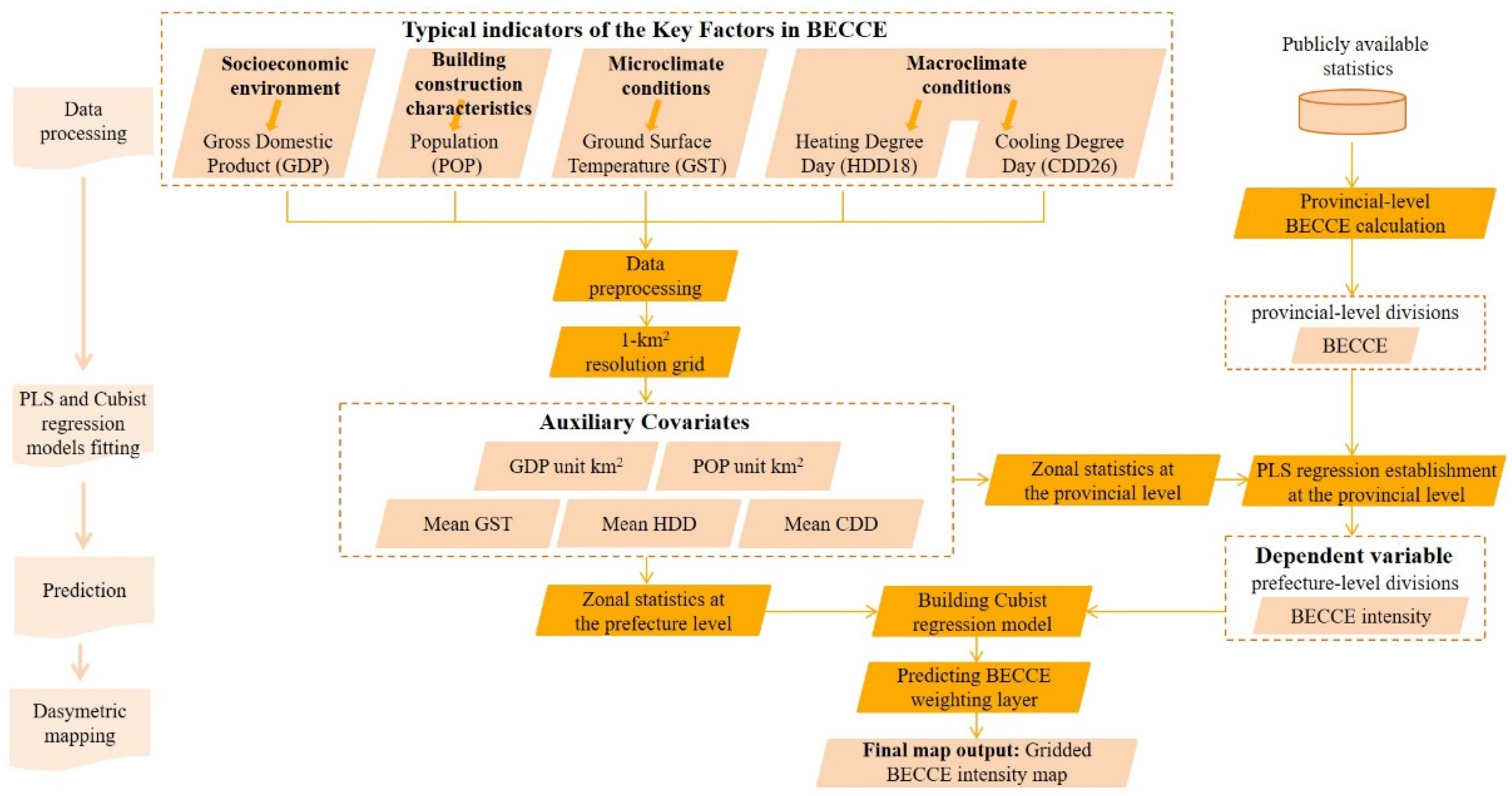
Figure 2.
Provincial grouping based on China’s building climate demarcation.
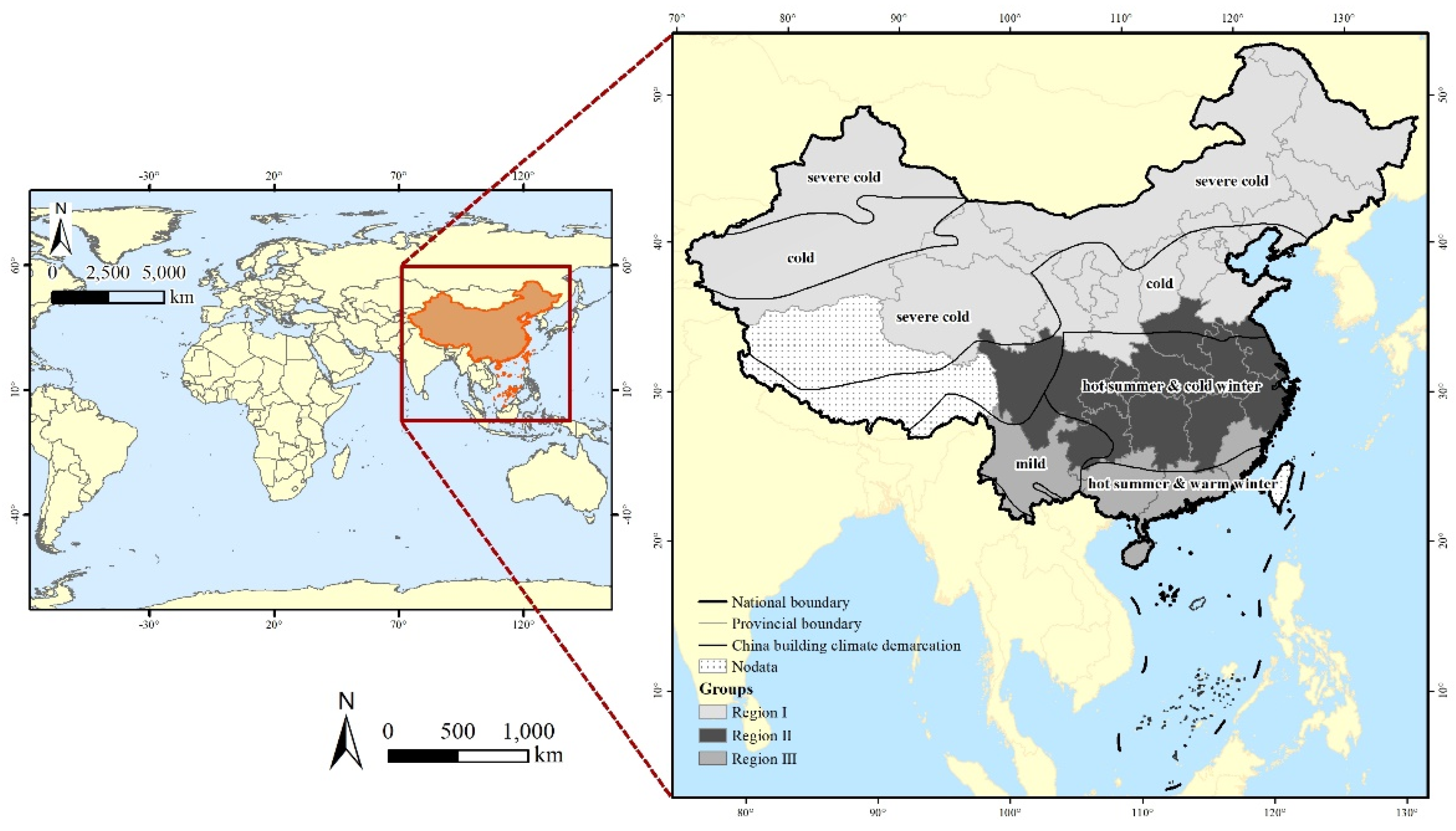
Figure 3.
Spatial distribution of GDP, POP, GST, HDD18, and CDD26 of China in 2015.
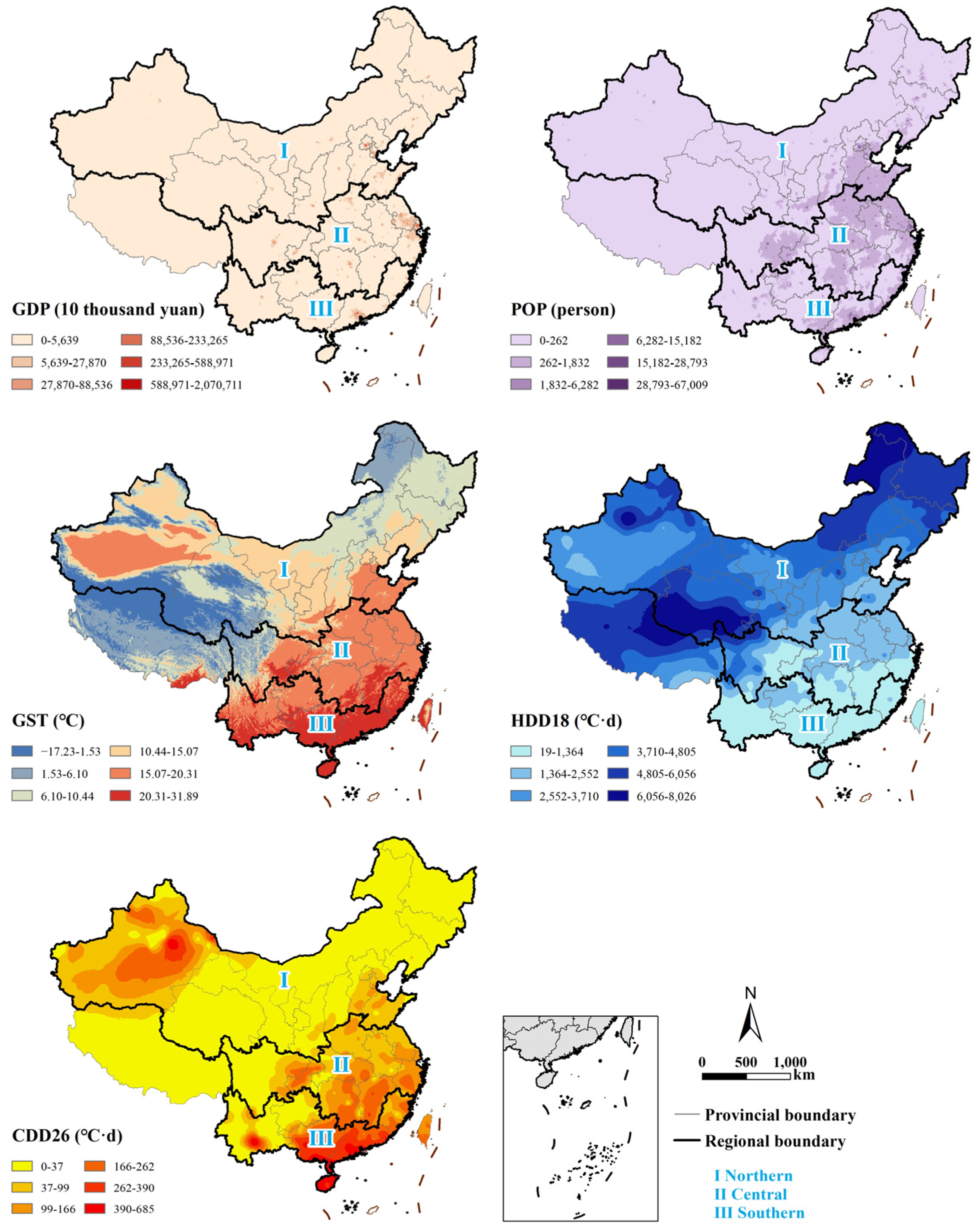
Figure 4.
Provincial-level BECCE of China in 2015.

Figure 5.
(a) Energy usage and resulting BECCE, and (b) BECCE from public buildings and residential buildings in China (unit: ×104 tons of CO2).
Figure 5.
(a) Energy usage and resulting BECCE, and (b) BECCE from public buildings and residential buildings in China (unit: ×104 tons of CO2).
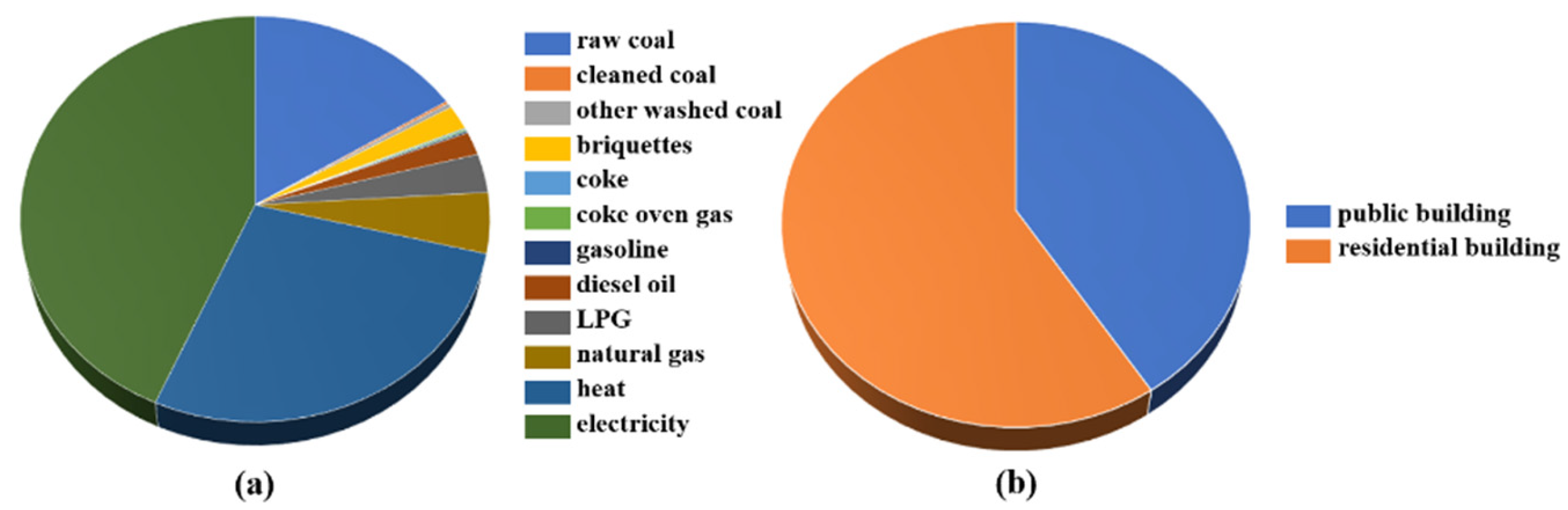
Figure 6.
Prefectural-level BECCE of China in 2015.
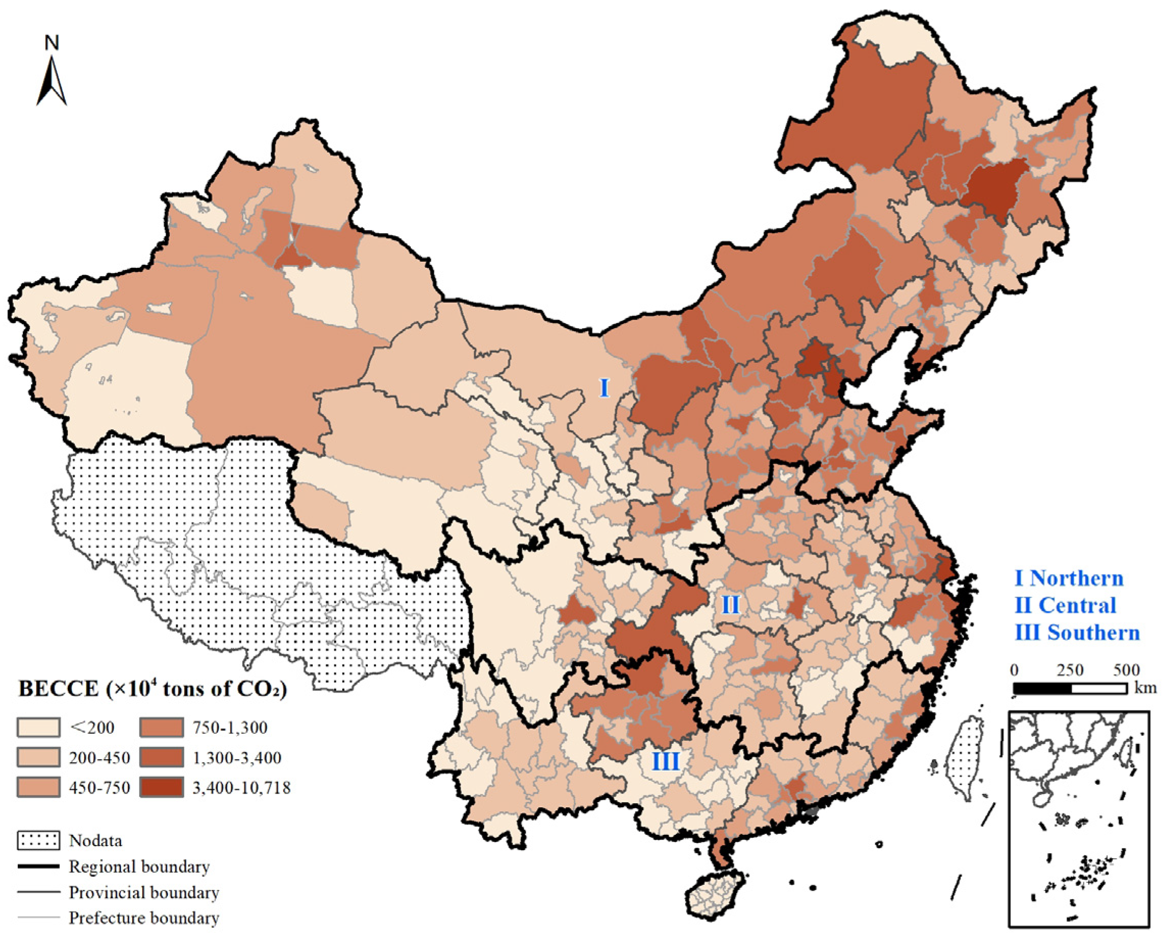
Figure 7.
Map of estimated BECCE intensity of China in 2015.
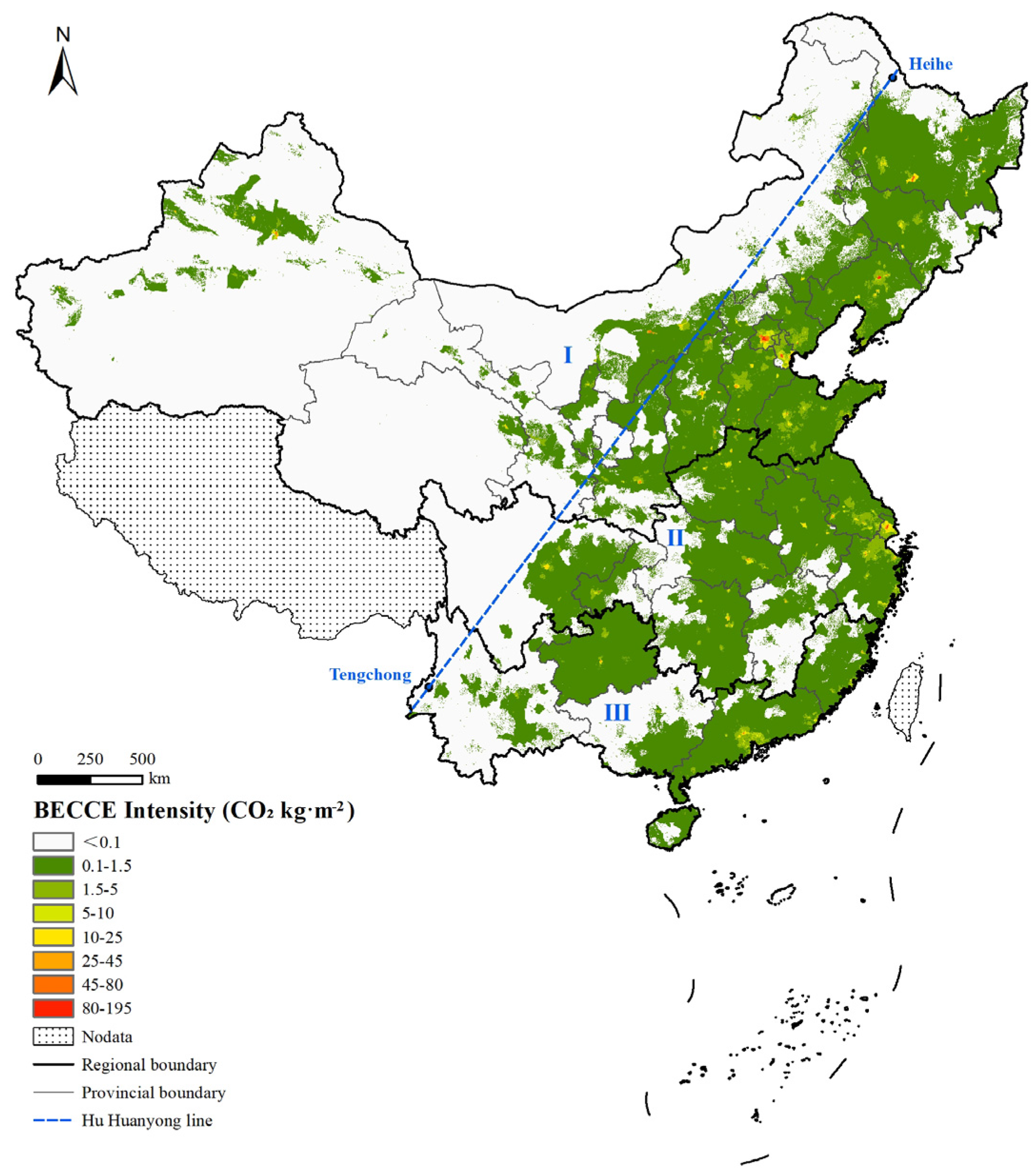
Figure 8.
Importance of covariates in the Cubist regression models for estimation of BECCE intensity: (a) region I, (b) region II, and (c) region III.
Figure 8.
Importance of covariates in the Cubist regression models for estimation of BECCE intensity: (a) region I, (b) region II, and (c) region III.
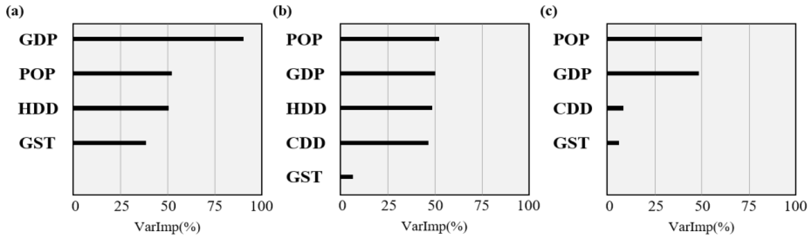
Figure 9.
Comparison of normalized BECCE intensity and AHFb for eight metropolitan cities in China.
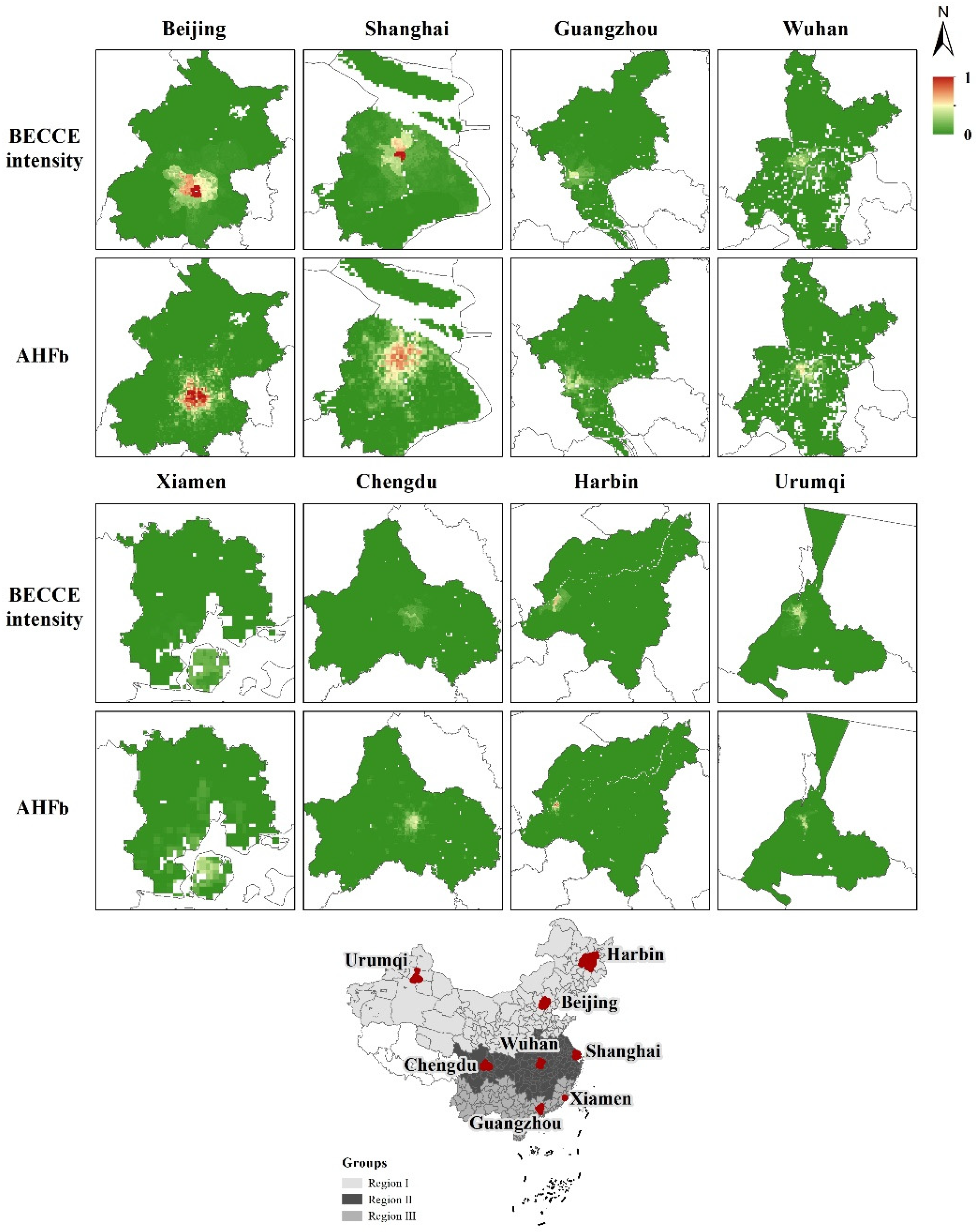
Table 1.
PLS regression models constructed for each region (BECCE intensity labeled BECCEI).
| Groups | PLS Regression Models | Adjusted R2 |
|---|---|---|
| Region I | BECCEI = 0.742 GDP + 0.220 POP + 0.045 GST + 1.855 HDD − 7.149 | 0.963 |
| Region II | BECCEI = 0.489 GDP + 0.699 POP + 0.001 GST + 0.188 HDD + 0.030 CDD − 1.573 | 0.961 |
| Region III | BECCEI = 0.335 GDP + 0.520 POP + 0.013 GST + 0.174 CDD − 0.677 | 0.804 |
Table 2.
Results of Pearson correlation analysis between estimated BECCE intensity (labeled BECCEI) and AHFb.
Table 2.
Results of Pearson correlation analysis between estimated BECCE intensity (labeled BECCEI) and AHFb.
| Data for Assessment | Number of Samples | Regression Models | Pearson’s R |
|---|---|---|---|
| Whole | 8,155,038 | AHFb = 0.184 BECCEI + 0.007 | 0.620 ** |
| Region I | 5,422,939 | AHFb = 0.176 BECCEI + 0.004 | 0.644 ** |
| Region II | 1,614,474 | AHFb = 0.201 BECCEI + 0.012 | 0.601 ** |
| Region III | 1,117,625 | AHFb = 0.268 BECCEI – 0.006 | 0.526 ** |
** Correlation significant at the 0.01 level.
Publisher’s Note: MDPI stays neutral with regard to jurisdictional claims in published maps and institutional affiliations. |
© 2021 by the authors. Licensee MDPI, Basel, Switzerland. This article is an open access article distributed under the terms and conditions of the Creative Commons Attribution (CC BY) license (https://creativecommons.org/licenses/by/4.0/).
Share and Cite
MDPI and ACS Style
Zhao, Z.; Yang, X.; Yan, H.; Huang, Y.; Zhang, G.; Lin, T.; Ye, H. Downscaling Building Energy Consumption Carbon Emissions by Machine Learning. Remote Sens. 2021, 13, 4346. https://doi.org/10.3390/rs13214346
AMA Style
Zhao Z, Yang X, Yan H, Huang Y, Zhang G, Lin T, Ye H. Downscaling Building Energy Consumption Carbon Emissions by Machine Learning. Remote Sensing. 2021; 13(21):4346. https://doi.org/10.3390/rs13214346
Chicago/Turabian StyleZhao, Zhuoqun, Xuchao Yang, Han Yan, Yiyi Huang, Guoqin Zhang, Tao Lin, and Hong Ye. 2021. "Downscaling Building Energy Consumption Carbon Emissions by Machine Learning" Remote Sensing 13, no. 21: 4346. https://doi.org/10.3390/rs13214346
Note that from the first issue of 2016, this journal uses article numbers instead of page numbers. See further details here.