
A Meta-Analysis on Harmful Algal Bloom (HAB) Detection and Monitoring: A Remote Sensing Perspective

 ,
,  ,
,  ,
, 

Abstract

1. Introduction
2. Materials and Methods
3. Results
3.1. General Characteristics of Published Articles
3.2. Methods for HAB Detection and Monitoring
3.2.1. Scale of the Study
3.2.2. HAB Proxies
3.2.3. HAB Proxy Estimation Methods
3.2.4. Validation for HAB Proxy Estimation Methods
3.3. Sensors for HAB Monitoring
3.4. Sensor Resolutions
3.5. Processing Levels of Imagery
3.6. Ancillary Data
3.7. Software Environemnts Used
4. Discussion
4.1. General Characteristics
4.2. Reference Data
4.3. HAB Proxy Estimation Methods
4.4. Sensors for HAB Monitoring
4.5. Processing Levels of Remotely Sensed Imagery
4.6. Remote Sensing Data Resolutions
4.7. Ancillary Data
4.8. Software Environments Used
5. Challenges and Future Directions
6. Conclusions
- The number of published studies show an increasing trend, especially in USA and China. These studies were published in a wide range of journals indicating the diverse backgrounds of the researchers. Furthermore, evaluation metrics such as the number of citations and journal impact factor showed that the quality of HAB-related studies has also increased along with the quantity. However, the studies were not distributed around the globe hence there is need to evaluate other potential at-risk aquatic bodies to have a coherent picture about HABs.
- The most frequently used multispectral sensors were MODIS, SeaWiFS, MERIS, and Landsat-based sensors TM/ETM+/OLI. Though the launch of the Sentinel series is recent, a significant number of studies were utilizing MSI and OLCI datasets. About 75% of the studies were conducted over a longer temporal scale indicating the importance of continuous monitoring of HABs. These studies have utilized multiple sensors to generate a continuous temporal dataset.
- Data with various resolutions were used for different types of study areas. However, we can provide some generalization in that high spatial resolution data are more common for smaller study areas such as inland waters, and low spatial resolution data are used for larger study areas such as coastal bodies and open waters. A tradeoff between resolutions is generally observed, therefore a virtual constellation of satellites and data fusion is recommended to fill the data gaps and improve the accuracy. The geostationary satellites have been proven useful for monitoring of HABs as they have greater temporal resolution. Experiments with CubeSats such as Planetscope have also revealed their potential for HAB detection and monitoring. However, further studies are required in order to draw a concrete conclusion.
- Among the data processing levels, level 1 was most frequently used as it maximizes flexibility to customize the preprocessing steps. Studies used multiple atmospheric correction methods; however, no standard model was observed. Hence, a suitable atmospheric correction model especially for turbid waters having low HAB proxy concentrations is still an active area of research.
- In terms of HAB proxies, studies mostly modeled chlorophyll using airborne and spaceborne data. Although phycocyanin has distinct spectral features, the unavailability of phycocyanin pigment in routine water quality measuring projects makes it difficult to calibrate with the remotely-sensed Earth observation data. There is also a need to focus more on using FLH and cell densities to discriminate different phytoplankton groups.
- There are multiple sources of ancillary data that are used in conjunction with HAB proxies. The most frequently used, particularly in the case of oceanic waters were SST, wind vector, and SSHA data. These ancillary data help in understanding the seasonal variations of HABs and potential causes behind those variations. For coastal and reservoir waters, ancillary data such as TSM, turbidity, and hydrological parameters were used. These data help in understanding the sources and movements of sediments that cause turbidity in water. Further research is needed to understand the relation between turbidity and the generation of HABs.
- There are various estimation methods for HAB proxies among which the regression-based methods outperform the spectral based methods. However, the performance comparison of regression models with analytical models was inconclusive. Therefore, further research is needed as the performance varied on a case-by-case basis. The models’ performance depends on multiple factors such as the quantity and quality of ground-based data, in situ reflectance, preprocessing steps, sensor specifications and the type of water body. There is a need for standardized reporting of methodology to make direct comparisons between studies. Furthermore, the various accuracy assessment metrics also limit cross-study comparison. However, in terms of validation, regression-based models generally used R2 and RMSE while overall accuracy and kappa coefficient were used for classification-based methods.
- The most frequently used processing software was SeaDAS. Generally, there was greater use of GUI-based environments as compared to programming based. However, over the last few years, more studies were using cloud-computing platforms such as GEE for broad-scale HAB detection and monitoring. GEE is also being used to develop applications for real-time HABs detection.
- For future work, there is still a need to utilize machine learning algorithms not only for detection but for time series analysis as well. The utilization of analytical methods along with satellite imagery is still an open area of research.
- The upcoming satellites such as Landsat 9 and NASA’s hyperspectral satellites will open multiple avenues of research for HAB monitoring and detection. These datasets will help in species discrimination and can be useful for the detection of the vertical movement of HABs.
Author Contributions
Funding
Institutional Review Board Statement
Informed Consent Statement
Data Availability Statement
Conflicts of Interest
References
- Anderson, C.R.; Moore, S.K.; Tomlinson, M.C.; Silke, J.; Cusack, C.K. Living with Harmful Algal Blooms in a Changing World. In Coastal and Marine Hazards, Risks, and Disasters; Elsevier: Amsterdam, The Netherlands, 2015; pp. 495–561. ISBN 978-0-12-396483-0. [Google Scholar]
- Roelke, D.; Buyukates, Y. The Diversity of Harmful Algal Bloom-Triggering Mechanisms and the Complexity of Bloom Initiation. Hum. Ecol. Risk Assess. Int. J. 2001, 7, 1347–1362. [Google Scholar] [CrossRef]
- Smayda, T.J. Harmful algal blooms: Their ecophysiology and general relevance to phytoplankton blooms in the sea. Limnol. Oceanogr. 1997, 42, 1137–1153. [Google Scholar] [CrossRef]
- Fogg, G.E. Harmful algae—A perspective. Harmful Algae 2002, 1, 1–4. [Google Scholar] [CrossRef]
- Heisler, J.; Glibert, P.M.; Burkholder, J.M.; Anderson, D.M.; Cochlan, W.; Dennison, W.C.; Dortch, Q.; Gobler, C.J.; Heil, C.A.; Humphries, E.; et al. Eutrophication and harmful algal blooms: A scientific consensus. Harmful Algae 2008, 8, 3–13. [Google Scholar] [CrossRef]
- Hallegraeff, G.M. A review of harmful algal blooms and their apparent global increase. Phycologia 1993, 32, 79–99. [Google Scholar] [CrossRef]
- Hallegraeff, G.M. Ocean climate change, phytoplankton community responses, and harmful algal blooms: A formidable predictive challenge. J. Phycol. 2010, 46, 220–235. [Google Scholar] [CrossRef]
- Ahn, Y.-H.; Shanmugam, P. Detecting the red tide algal blooms from satellite ocean color observations in optically complex Northeast-Asia Coastal waters. Remote Sens. Environ. 2006, 103, 419–437. [Google Scholar] [CrossRef]
- Carmichael, W.W.; Boyer, G.L. Health impacts from cyanobacteria harmful algae blooms: Implications for the North American Great Lakes. Harmful Algae 2016, 54, 194–212. [Google Scholar] [CrossRef]
- Lapointe, B.E.; Herren, L.W.; Debortoli, D.D.; Vogel, M.A. Evidence of sewage-driven eutrophication and harmful algal blooms in Florida’s Indian River Lagoon. Harmful Algae 2015, 43, 82–102. [Google Scholar] [CrossRef]
- Tang, D.L.; Kawamura, H.; Doan-Nhu, H.; Takahashi, W. Remote sensing oceanography of a harmful algal bloom off the coast of southeastern Vietnam: Oceanography of a hab off vietnam coast. J. Geophys. Res. 2004, 109. [Google Scholar] [CrossRef]
- Paerl, H.W.; Huisman, J. Climate: Blooms Like It Hot. Science 2008, 320, 57–58. [Google Scholar] [CrossRef]
- Tester, P.A.; Steidinger, K.A. Gymnodinium breve red tide blooms: Initiation, transport, and consequences of surface circulation. Limnol. Oceanogr. 1997, 42, 1039–1051. [Google Scholar] [CrossRef]
- Kahru, M.; Aitsam, A.; Elken, J. Coarse-Scale Spatial Structure of Phytoplankton Standing Crop in Relation to Hydrography in the Open Baltic Sea. Mar. Ecol. Prog. Ser. 1981, 5, 311–318. [Google Scholar] [CrossRef]
- Kononen, K.; Kuparinen, J.; Mäkelä, K.; Laanemets, J.; Pavelson, J.; Nõmmann, S. Initiation of cyanobacterial blooms in a frontal region at the entrance to the Gulf of Finland, Baltic Sea. Limnol. Oceanogr. 1996, 41, 98–112. [Google Scholar] [CrossRef]
- Lindsey, R.; Scott, M. What Are Phytoplankton? Available online: https://earthobservatory.nasa.gov/features/Phytoplankton (accessed on 23 September 2021).
- Zingone, A.; Oksfeldt Enevoldsen, H. The diversity of harmful algal blooms: A challenge for science and management. Ocean. Coast. Manag. 2000, 43, 725–748. [Google Scholar] [CrossRef]
- Horner, R.A.; Garrison, D.L.; Plumley, F.G. Harmful algal blooms and red tide problems on the U.S. west coast. Limnol. Oceanogr. 1997, 42, 1076–1088. [Google Scholar] [CrossRef]
- Shumway, S.E.; Barter, J.; Sherman-Caswell, S. Auditing the impact of toxic algal blooms on oysters. Environ. Audit. 1990, 2, 41–56. [Google Scholar]
- Paerl, H.W. Nuisance phytoplankton blooms in coastal, estuarine, and inland waters1: Nuisance blooms. Limnol. Oceanogr. 1988, 33, 823–843. [Google Scholar] [CrossRef]
- Salas, R.; Tillmann, U.; John, U.; Kilcoyne, J.; Burson, A.; Cantwell, C.; Hess, P.; Jauffrais, T.; Silke, J. The role of Azadinium spinosum (Dinophyceae) in the production of azaspiracid shellfish poisoning in mussels. Harmful Algae 2011, 10, 774–783. [Google Scholar] [CrossRef]
- Amzil, Z.; Sibat, M.; Chomerat, N.; Grossel, H.; Marco-Miralles, F.; Lemee, R.; Nezan, E.; Sechet, V. Ovatoxin-a and Palytoxin Accumulation in Seafood in Relation to Ostreopsis cf. ovata Blooms on the French Mediterranean Coast. Mar. Drugs 2012, 10, 477–496. [Google Scholar] [CrossRef]
- Ho, J.C.; Michalak, A.M.; Pahlevan, N. Widespread global increase in intense lake phytoplankton blooms since the 1980s. Nature 2019, 574, 667–670. [Google Scholar] [CrossRef]
- Rodríguez-Benito, C.V.; Navarro, G.; Caballero, I. Using Copernicus Sentinel-2 and Sentinel-3 data to monitor harmful algal blooms in Southern Chile during the COVID-19 lockdown. Mar. Pollut. Bull. 2020, 161, 111722. [Google Scholar] [CrossRef]
- Dierssen, H.M.; Kudela, R.M.; Ryan, J.P.; Zimmerman, R.C. Red and black tides: Quantitative analysis of water-leaving radiance and perceived color for phytoplankton, colored dissolved organic matter, and suspended sediments. Limnol. Oceanogr. 2006, 51, 2646–2659. [Google Scholar] [CrossRef]
- Gobler, C.J.; Sunda, W.G. Ecosystem disruptive algal blooms of the brown tide species, Aureococcus anophagefferens and Aureoumbra lagunensis. Harmful Algae 2012, 14, 36–45. [Google Scholar] [CrossRef]
- Dolah, F.M.V.; Roelke, D.; Greene, R.M. Health and Ecological Impacts of Harmful Algal Blooms: Risk Assessment Needs. Hum. Ecol. Risk Assess. Int. J. 2001, 7, 1329–1345. [Google Scholar] [CrossRef]
- Sekula-Wood, E.; Schnetzer, A.; Benitez-Nelson, C.R.; Anderson, C.; Berelson, W.M.; Brzezinski, M.A.; Burns, J.M.; Caron, D.A.; Cetinic, I.; Ferry, J.L.; et al. Rapid downward transport of the neurotoxin domoic acid in coastal waters. Nat. Geosci. 2009, 2, 272–275. [Google Scholar] [CrossRef]
- Paerl, H.W.; Hall, N.S.; Calandrino, E.S. Controlling harmful cyanobacterial blooms in a world experiencing anthropogenic and climatic-induced change. Sci. Total Environ. 2011, 409, 1739–1745. [Google Scholar] [CrossRef] [PubMed]
- Pick, F.R. Blooming algae: A Canadian perspective on the rise of toxic cyanobacteria. Can. J. Fish. Aquat. Sci. 2016, 73, 1149–1158. [Google Scholar] [CrossRef]
- Ndlela, L.L.; Oberholster, P.J.; Van Wyk, J.H.; Cheng, P.H. An overview of cyanobacterial bloom occurrences and research in Africa over the last decade. Harmful Algae 2016, 60, 11–26. [Google Scholar] [CrossRef] [PubMed]
- Dyson, K.; Huppert, D.D. Regional economic impacts of razor clam beach closures due to harmful algal blooms (HABs) on the Pacific coast of Washington. Harmful Algae 2010, 9, 264–271. [Google Scholar] [CrossRef]
- Imai, I.; Yamaguchi, M.; Hori, Y. Eutrophication and occurrences of harmful algal blooms in the Seto Inland Sea, Japan. Plankton Benthos Res. 2006, 1, 71–84. [Google Scholar] [CrossRef]
- Jin, D.; Hoagland, P. The value of harmful algal bloom predictions to the nearshore commercial shellfish fishery in the Gulf of Maine. Harmful Algae 2008, 7, 772–781. [Google Scholar] [CrossRef]
- Anderson, D.M. Approaches to monitoring, control and management of harmful algal blooms (HABs). Ocean. Coast. Manag. 2009, 52, 342–347. [Google Scholar] [CrossRef] [PubMed]
- Anderson, D.M.; Hoagland, P.; Kaoru, Y.; White, A.W. Estimated Annual Economic Impacts from Harmful Algal Blooms (HABs) in the United States; Woods Hole Oceanographic Institution: Woods Hole, MA, USA, 2000. [Google Scholar]
- Paerl, H.W.; Gardner, W.S.; Havens, K.E.; Joyner, A.R.; McCarthy, M.J.; Newell, S.E.; Qin, B.; Scott, J.T. Mitigating cyanobacterial harmful algal blooms in aquatic ecosystems impacted by climate change and anthropogenic nutrients. Harmful Algae 2016, 54, 213–222. [Google Scholar] [CrossRef]
- Glibert, P.M.; Harrison, J.; Heil, C.; Seitzinger, S. Escalating Worldwide use of Urea—A Global Change Contributing to Coastal Eutrophication. Biogeochemistry 2006, 77, 441–463. [Google Scholar] [CrossRef]
- Anderson, D.M.; Glibert, P.M.; Burkholder, J.M. Harmful algal blooms and eutrophication: Nutrient sources, composition, and consequences. Estuaries 2002, 25, 704–726. [Google Scholar] [CrossRef]
- Anderson, D.M.; Burkholder, J.M.; Cochlan, W.P.; Glibert, P.M.; Gobler, C.J.; Heil, C.A.; Kudela, R.M.; Parsons, M.L.; Rensel, J.E.J.; Townsend, D.W.; et al. Harmful algal blooms and eutrophication: Examining linkages from selected coastal regions of the United States. Harmful Algae 2008, 8, 39–53. [Google Scholar] [CrossRef]
- Randolph, K.; Wilson, J.; Tedesco, L.; Li, L.; Pascual, D.L.; Soyeux, E. Hyperspectral remote sensing of cyanobacteria in turbid productive water using optically active pigments, chlorophyll a and phycocyanin. Remote Sens. Environ. 2008, 112, 4009–4019. [Google Scholar] [CrossRef]
- Hunter, P.D.; Tyler, A.N.; Gilvear, D.J.; Willby, N.J. Using Remote Sensing to Aid the Assessment of Human Health Risks from Blooms of Potentially Toxic Cyanobacteria. Environ. Sci. Technol. 2009, 43, 2627–2633. [Google Scholar] [CrossRef]
- Richardson, L.L. Remote Sensing of Algal Bloom Dynamics. BioScience 1996, 46, 492–501. [Google Scholar] [CrossRef]
- Kutser, T. Passive optical remote sensing of cyanobacteria and other intense phytoplankton blooms in coastal and inland waters. Int. J. Remote Sens. 2009, 30, 4401–4425. [Google Scholar] [CrossRef]
- Chapman, D.J.; Chapman, V.J. The Algae; Springer: Berlin/Heidelberg, Germany, 1973. [Google Scholar]
- Reinart, A.; Kutser, T. Comparison of different satellite sensors in detecting cyanobacterial bloom events in the Baltic Sea. Remote Sens. Environ. 2006, 102, 74–85. [Google Scholar] [CrossRef]
- Ruiz-Verdú, A.; Simis, S.G.H.; de Hoyos, C.; Gons, H.J.; Peña-Martínez, R. An evaluation of algorithms for the remote sensing of cyanobacterial biomass. Remote Sens. Environ. 2008, 112, 3996–4008. [Google Scholar] [CrossRef]
- Duan, W.; He, B.; Takara, K.; Luo, P.; Nover, D.; Sahu, N.; Yamashiki, Y. Spatiotemporal evaluation of water quality incidents in Japan between 1996 and 2007. Chemosphere 2013, 93, 946–953. [Google Scholar] [CrossRef]
- Kallio, K. Remote sensing as a tool for monitoring lake water quality. Hydrol. Limnol. Asp. Lake Monit. 2000, 14, 237. [Google Scholar]
- Allee, R.J.; Johnson, J.E. Use of satellite imagery to estimate surface chlorophyll a and Secchi disc depth of Bull Shoals Reservoir, Arkansas, USA. Int. J. Remote Sens. 1999, 20, 1057–1072. [Google Scholar] [CrossRef]
- Hu, C.; Lee, Z.; Ma, R.; Yu, K.; Li, D.; Shang, S. Moderate Resolution Imaging Spectroradiometer (MODIS) observations of cyanobacteria blooms in Taihu Lake, China. J. Geophys. Res. Ocean. 2010, 115. [Google Scholar] [CrossRef]
- Pahlevan, N.; Smith, B.; Schalles, J.; Binding, C.; Cao, Z.; Ma, R.; Alikas, K.; Kangro, K.; Gurlin, D.; Ha, N.; et al. Seamless retrievals of chlorophyll-a from Sentinel-2 (MSI) and Sentinel-3 (OLCI) in inland and coastal waters: A machine-learning approach. Remote Sens. Environ. 2020, 240, 111604. [Google Scholar] [CrossRef]
- Tomlinson, M.C.; Stumpf, R.P.; Ransibrahmanakul, V.; Truby, E.W.; Kirkpatrick, G.J.; Pederson, B.A.; Vargo, G.A.; Heil, C.A. Evaluation of the use of SeaWiFS imagery for detecting Karenia brevis harmful algal blooms in the eastern Gulf of Mexico. Remote Sens. Environ. 2004, 91, 293–303. [Google Scholar] [CrossRef]
- Dekker, A.; Malthus, T.; Wijnen, M.; Seyhan, E. Remote sensing as a tool for assessing water quality in Loosdrecht lakes. Hydrobiologia 1992, 233, 137–159. [Google Scholar] [CrossRef]
- Dekker, A.G. Detection of Optical Water Quality Parameters for Eutrophic Waters by High Resolution Remote Sensing. Ph.D. Thesis, Vrije Universiteit Amsterdam, Vrije, The Amsterdam, 1993. [Google Scholar]
- Simis, S.G.H.; Ruiz-Verdú, A.; Domínguez-Gómez, J.A.; Peña-Martinez, R.; Peters, S.W.M.; Gons, H.J. Influence of phytoplankton pigment composition on remote sensing of cyanobacterial biomass. Remote Sens. Environ. 2007, 106, 414–427. [Google Scholar] [CrossRef]
- Simis, S.G.H.; Peters, S.W.M.; Gons, H.J. Remote sensing of the cyanobacterial pigment phycocyanin in turbid inland water. Limnol. Oceanogr. 2005, 50, 237–245. [Google Scholar] [CrossRef]
- Loisel, H.; Vantrepotte, V.; Ouillon, S.; Ngoc, D.D.; Herrmann, M.; Tran, V.; Meriaux, X.; Dessailly, D.; Jamet, C.; Duhaut, T.; et al. Assessment and analysis of the chlorophyll-a concentration variability over the Vietnamese coastal waters from the MERIS ocean color sensor (2002–2012). Remote Sens. Environ. 2017, 190, 217–232. [Google Scholar] [CrossRef]
- Vincent, R.K.; Qin, X.M.; McKay, R.M.L.; Miner, J.; Czajkowski, K.; Savino, J.; Bridgeman, T. Phycocyanin detection from LANDSAT TM data for mapping cyanobacterial blooms in Lake Erie. Remote Sens. Environ. 2004, 89, 381–392. [Google Scholar] [CrossRef]
- Werdell, P.J.; Bailey, S.W.; Franz, B.A.; Harding, L.W., Jr.; Feldman, G.C.; McClain, C.R. Regional and seasonal variability of chlorophyll-a in Chesapeake Bay as observed by SeaWiFS and MODIS-Aqua. Remote Sens. Environ. 2009, 113, 1319–1330. [Google Scholar] [CrossRef]
- Hu, C.M.; Muller-Karger, F.E.; Taylor, C.; Carder, K.L.; Kelble, C.; Johns, E.; Heil, C.A. Red tide detection and tracing using MODIS fluorescence data: A regional example in SW Florida coastal waters. Remote Sens. Environ. 2005, 97, 311–321. [Google Scholar] [CrossRef]
- Lee, M.-S.; Park, K.-A.; Chae, J.; Park, J.-E.; Lee, J.-S.; Lee, J.-H. Red tide detection using deep learning and high-spatial resolution optical satellite imagery. Int. J. Remote Sens. 2020, 41, 5838–5860. [Google Scholar] [CrossRef]
- Gohin, F.; der Zande, D.; Tilstone, G.; Eleveld, M.A.; Lefebvre, M.; Andrieux-Loyer, F.; Blauw, A.N.; Bryere, P.; Devreker, D.; Gamesson, P.; et al. Twenty years of satellite and in situ observations of surface chlorophyll-a from the northern Bay of Biscay to the eastern English Channel. Is the water quality improving? Remote Sens. Environ. 2019, 233, 111343. [Google Scholar] [CrossRef]
- Palmer, S.C.J.; Odermatt, D.; Hunter, P.D.; Brockmann, C.; Presing, M.; Balzter, H.; Toth, V.R. Satellite remote sensing of phytoplankton phenology in Lake Balaton using 10 years of MERIS observations. Remote Sens. Environ. 2015, 158, 441–452. [Google Scholar] [CrossRef]
- Vantrepotte, V.; Melin, F. Inter-annual variations in the SeaWiFS global chlorophyll a concentration (1997–2007). Deep. Sea Res. Part I Oceanogr. Res. Pap. 2011, 58, 429–441. [Google Scholar] [CrossRef]
- Gholizadeh, M.; Melesse, A.; Reddi, L. A Comprehensive Review on Water Quality Parameters Estimation Using Remote Sensing Techniques. Sensors 2016, 16, 1298. [Google Scholar] [CrossRef] [PubMed]
- Bryant, D.A. The Photoregulated Expression of Multiple Phycocyanin Species. A General Mechanism for the Control of Phycocyanin Synthesis is Chromatically Adapting Cyanobacteria. Eur. J. Biochem. 1981, 119, 425–429. [Google Scholar] [CrossRef]
- Ogashawara, I.; Mishra, D.; Mishra, S.; Curtarelli, M.; Stech, J. A Performance Review of Reflectance Based Algorithms for Predicting Phycocyanin Concentrations in Inland Waters. Remote Sens. 2013, 5, 4774–4798. [Google Scholar] [CrossRef]
- Dekker, A.G.; Malthus, T.J.; Seyhan, E. Quantitative modeling of inland water quality for high-resolution MSS systems. IEEE Trans. Geosci. Remote Sens. 1991, 29, 89–95. [Google Scholar] [CrossRef]
- Kutser, T. Quantitative detection of chlorophyll in cyanobacterial blooms by satellite remote sensing. Limnol. Oceanogr. 2004, 49, 2179–2189. [Google Scholar] [CrossRef]
- Sathyendranath, S.; Lazzara, L.; Prieur, L. Variations in the spectral values of specific absorption of phytoplankton: Phytoplankton specific absorption. Limnol. Oceanogr. 1987, 32, 403–415. [Google Scholar] [CrossRef]
- Goodin, D.G.; Han, H.L.; Fraser, R.N.; Rundquist, D.C.; Stebbins, W.A.; Schalles, J.F. Analysis of suspended solids in water using remotely sensed high resolution derivative spectra. Photogramm. Eng. Remote Sens. 1993, 59, 505–510. [Google Scholar]
- Smith, R.C.; Tyler, J.E. Transmission of solar radiation into natural waters. In Photochemical and Photobiological Reviews; Springer: Berlin/Heidelberg, Germany, 1976; pp. 117–155. [Google Scholar]
- Sagan, V.; Peterson, K.T.; Maimaitijiang, M.; Sidike, P.; Sloan, J.; Greeling, B.A.; Maalouf, S.; Adams, C. Monitoring inland water quality using remote sensing: Potential and limitations of spectral indices, bio-optical simulations, machine learning, and cloud computing. Earth Sci. Rev. 2020, 205, 103187. [Google Scholar] [CrossRef]
- Morel, A.; Prieur, L. Analysis of variations in ocean color1: Ocean color analysis. Limnol. Oceanogr. 1977, 22, 709–722. [Google Scholar] [CrossRef]
- Haji Gholizadeh, M.; Melesse, A.M.; Reddi, L. Spaceborne and airborne sensors in water quality assessment. Int. J. Remote Sens. 2016, 37, 3143–3180. [Google Scholar] [CrossRef]
- Gitelson, A.; Mayo, M.; Yacobi, Y.Z.; Parparov, A.; Berman, T. The use of high-spectral-resolution radiometer data for detection of chlorophyll concentrations in Lake Kinneret. J. Plankton Res. 1994, 10, 993–1002. [Google Scholar] [CrossRef]
- Gower, J.F.R.; Brown, L.; Borstad, G.A. Observation of chlorophyll fluorescence in west coast waters of Canada using the MODIS satellite sensor. Can. J. Remote Sens. 2004, 30, 9. [Google Scholar] [CrossRef]
- Matthews, M.W. Eutrophication and cyanobacterial blooms in South African inland waters: 10 years of MERIS observations. Remote Sens. Environ. 2014, 155, 161–177. [Google Scholar] [CrossRef]
- Roelfsema, C.M.; Phinn, S.R.; Dennison, W.C.; Dekker, A.G.; Brando, V.E. Monitoring toxic cyanobacteria Lyngbya majuscula (Gomont) in Moreton Bay, Australia by integrating satellite image data and field mapping. Harmful Algae 2006, 5, 45–56. [Google Scholar] [CrossRef]
- Xu, M.; Liu, H.; Beck, R.; Lekki, J.; Yang, B.; Shu, S.; Kang, E.L.; Anderson, R.; Johansen, R.; Emery, E.; et al. A spectral space partition guided ensemble method for retrieving chlorophyll-a concentration in inland waters from Sentinel-2A satellite imagery. J. Great Lakes Res. 2019, 45, 454–465. [Google Scholar] [CrossRef]
- Doernhoefer, K.; Klinger, P.; Heege, T.; Oppelt, N. Multi-sensor satellite and in situ monitoring of phytoplankton development in a eutrophic-mesotrophic lake. Sci. Total. Environ. 2018, 612, 1200–1214. [Google Scholar] [CrossRef]
- Wu, D.; Li, R.; Zhang, F.; Liu, J. A review on drone-based harmful algae blooms monitoring. Environ. Monit. Assess. 2019, 191, 211. [Google Scholar] [CrossRef]
- Lomax, A.S.; Corso, W.; Etro, J.F. Employing Unmanned Aerial Vehicles (UAVs) as an Element of the Integrated Ocean Observing System. In Proceedings of the OCEANS 2005 MTS/IEEE, Washington, DC, USA, 17–23 September 2005; pp. 1–7. [Google Scholar]
- Kislik, C.; Dronova, I.; Kelly, M. UAVs in Support of Algal Bloom Research: A Review of Current Applications and Future Opportunities. Drones 2018, 2, 35. [Google Scholar] [CrossRef]
- Bak, S.-H.; Kim, H.-M.; Hwang, D.-H.; Oh, S.-Y.; Yoon, H.-J. Red Tide Detection Technique by Using Multi-temporal GOCI Level 2 Data. Int. J. Grid Distrib. Comput. 2017, 10, 45–55. [Google Scholar] [CrossRef]
- Bresciani, M.; Adamo, M.; De Carolis, G.; Matta, E.; Pasquariello, G.; Vaiciute, D.; Giardino, C. Monitoring blooms and surface accumulation of cyanobacteria in the Curonian Lagoon by combining MERIS and ASAR data. Remote Sens. Environ. 2014, 146, 124–135. [Google Scholar] [CrossRef]
- Zhang, Y.; Hallikainen, M.; Zhang, H.; Duan, H.; Li, Y.; Liang, X.S. Chlorophyll-a Estimation in Turbid Waters Using Combined SAR Data with Hyperspectral Reflectance Data: A Case Study in Lake Taihu, China. IEEE J. Sel. Top. Appl. Earth Obs. Remote Sens. 2018, 11, 1325–1336. [Google Scholar] [CrossRef]
- Lunetta, R.S.; Schaeffer, B.A.; Stumpf, R.P.; Keith, D.; Jacobs, S.A.; Murphy, M.S. Evaluation of cyanobacteria cell count detection derived from MERIS imagery across the eastern USA. Remote Sens. Environ. 2015, 157, 24–34. [Google Scholar] [CrossRef]
- Torbick, N.; Hu, F.; Zhang, J.; Qi, J.; Zhang, H.; Becker, B. Mapping Chlorophyll-a Concentrations in West Lake, China using Landsat 7 ETM+. J. Great Lakes Res. 2008, 34, 559–565. [Google Scholar] [CrossRef]
- Le, C.; Hu, C.; English, D.; Cannizzaro, J.; Kovach, C. Climate-driven chlorophyll-a changes in a turbid estuary: Observations from satellites and implications for management. Remote Sens. Environ. 2013, 130, 11–24. [Google Scholar] [CrossRef]
- Korb, R.E.; Whitehouse, M.J.; Ward, P. SeaWiFS in the southern ocean: Spatial and temporal variability in phytoplankton biomass around South Georgia. Deep Sea Res. Part II Top. Stud. Oceanogr. 2004, 51, 99–116. [Google Scholar] [CrossRef]
- Moses, W.J.; Gitelson, A.A.; Berdnikov, S.; Saprygin, V.; Povazhnyi, V. Operational MERIS-based NIR-red algorithms for estimating chlorophyll-a concentrations in coastal waters—The Azov Sea case study. Remote Sens. Environ. 2012, 121, 118–124. [Google Scholar] [CrossRef]
- Siegel, D.A.; Behrenfeld, M.; Maritorena, S.; McClain, C.R.; Antoine, D.; Bailey, S.W.; Bontempi, P.S.; Boss, E.S.; Dierssen, H.M.; Doney, S.C.; et al. Regional to global assessments of phytoplankton dynamics from the SeaWiFS mission. Remote Sens. Environ. 2013, 135, 77–91. [Google Scholar] [CrossRef]
- Duan, H.; Zhang, Y.; Zhan, B.; Song, K.; Wang, Z. Assessment of chlorophyll-a concentration and trophic state for Lake Chagan using Landsat TM and field spectral data. Environ. Monit. Assess. 2007, 129, 295–308. [Google Scholar] [CrossRef]
- Qi, L.; Hu, C.; Duan, H.; Cannizzaro, J.; Ma, R. A novel MERIS algorithm to derive cyanobacterial phycocyanin pigment concentrations in a eutrophic lake: Theoretical basis and practical considerations. Remote Sens. Environ. 2014, 154, 298–317. [Google Scholar] [CrossRef]
- Carvalho, G.A.; Minnett, P.J.; Banzon, V.F.; Baringer, W.; Heil, C.A. Long-term evaluation of three satellite ocean color algorithms for identifying harmful algal blooms (Karenia brevis) along the west coast of Florida: A matchup assessment. Remote Sens. Environ. 2011, 115, 1–18. [Google Scholar] [CrossRef]
- Ishizaka, J.; Kitaura, Y.; Touke, Y.; Sasaki, H.; Tanaka, A.; Murakami, H.; Suzuki, T.; Matsuoka, K.; Nakata, H. Satellite detection of red tide in Ariake Sound, 1998–2001. J. Oceanogr. 2006, 62, 37–45. [Google Scholar] [CrossRef]
- Cairo, C.; Barbosa, C.; Lobo, F.; Novo, E.; Carlos, F.; Maciel, D.; Flores Junior, R.; Silva, E.; Curtarelli, V. Hybrid Chlorophyll-a Algorithm for Assessing Trophic States of a Tropical Brazilian Reservoir Based on MSI/Sentinel-2 Data. Remote Sens. 2020, 12, 40. [Google Scholar] [CrossRef]
- Binding, C.E.; Greenberg, T.A.; McCullough, G.; Watson, S.B.; Page, E. An analysis of satellite-derived chlorophyll and algal bloom indices on Lake Winnipeg. J. Great Lakes Res. 2018, 44, 436–446. [Google Scholar] [CrossRef]
- El-Alem, A.; Chokmani, K.; Laurion, I.; El-Adlouni, S.E. Comparative analysis of four models to estimate chlorophyll-a concentration in case-2 waters using MODerate resolution imaging spectroradiometer (MODIS) imagery. Remote Sens. 2012, 4, 2373–2400. [Google Scholar] [CrossRef]
- Prasad, S.; Saluja, R.; Garg, J.K. Assessing the efficacy of Landsat-8 OLI imagery derived models for remotely estimating chlorophyll-a concentration in the Upper Ganga River, India. Int. J. Remote Sens. 2020, 41, 2439–2456. [Google Scholar] [CrossRef]
- Rao, K.H.; Smitha, A.; Ali, M.M. A study on cyclone induced productivity in south-western Bay of Bengal during November-December 2000 using MODIS (SST and chlorophyll-a) and altimeter sea surface height observations. Indian J. Mar. Sci. 2006, 35, 153–160. [Google Scholar]
- Cazzaniga, I.; Bresciani, M.; Colombo, R.; Della Bella, V.; Padula, R.; Giardino, C. A comparison of Sentinel-3-OLCI and Sentinel-2-MSI-derived Chlorophyll-a maps for two large Italian lakes. Remote Sens. Lett. 2019, 10, 978–987. [Google Scholar] [CrossRef]
- Schaeffer, B.A.; Bailey, S.W.; Conmy, R.N.; Galvin, M.; Ignatius, A.R.; Johnston, J.M.; Keith, D.J.; Lunetta, R.S.; Parmar, R.; Stumpf, R.P.; et al. Mobile device application for monitoring cyanobacteria harmful algal blooms using Sentinel-3 satellite Ocean and Land Colour Instruments. Environ. Model. Softw. 2018, 109, 93–103. [Google Scholar] [CrossRef]
- Davidson, K.; Anderson, D.M.; Mateus, M.; Reguera, B.; Silke, J.; Sourisseau, M.; Maguire, J. Forecasting the risk of harmful algal blooms. Harmful Algae 2016, 53, 1–7. [Google Scholar] [CrossRef]
- Hardison, D.R.; Holland, W.C.; Currier, R.D.; Kirkpatrick, B.; Stumpf, R.; Fanara, T.; Burris, D.; Reich, A.; Kirkpatrick, G.J.; Litaker, R.W. HABscope: A tool for use by citizen scientists to facilitate early warning of respiratory irritation caused by toxic blooms of Karenia brevis. PLoS ONE 2019, 14, e0218489. [Google Scholar] [CrossRef]
- Mishra, D.R.; Kumar, A.; Ramaswamy, L.; Boddula, V.K.; Das, M.C.; Page, B.P.; Weber, S.J. CyanoTRACKER: A cloud-based integrated multi-platform architecture for global observation of cyanobacterial harmful algal blooms. Harmful Algae 2020, 96, 101828. [Google Scholar] [CrossRef]
- de Lobo, F.L.; Nagel, G.W.; Maciel, D.A.; de Carvalho, L.A.S.; Martins, V.S.; Barbosa, C.C.F.; de Novo, E.M.L.M. AlgaeMAp: Algae Bloom Monitoring Application for Inland Waters in Latin America. Remote Sens. 2021, 13, 2874. [Google Scholar] [CrossRef]
- Wang, X.; Yang, W. Water quality monitoring and evaluation using remote sensing techniques in China: A systematic review. Ecosyst. Health Sustain. 2019, 5, 47–56. [Google Scholar] [CrossRef]
- Xiong, Y.; Ran, Y.; Zhao, S.; Zhao, H.; Tian, Q. Remotely assessing and monitoring coastal and inland water quality in China: Progress, challenges and outlook. Crit. Rev. Environ. Sci. Technol. 2020, 50, 1266–1302. [Google Scholar] [CrossRef]
- Dube, T.; Mutanga, O.; Seutloali, K.; Adelabu, S.; Shoko, C. Water quality monitoring in sub-Saharan African lakes: A review of remote sensing applications. Afr. J. Aquat. Sci. 2015, 40, 1–7. [Google Scholar] [CrossRef]
- Matthews, M.W.; Bernard, S.; Winter, K. Remote sensing of cyanobacteria-dominant algal blooms and water quality parameters in Zeekoevlei, a small hypertrophic lake, using MERIS. Remote Sens. Environ. 2010, 114, 2070–2087. [Google Scholar] [CrossRef]
- Topp, S.N.; Pavelsky, T.M.; Jensen, D.; Simard, M.; Ross, M.R.V. Research Trends in the Use of Remote Sensing for Inland Water Quality Science: Moving Towards Multidisciplinary Applications. Water 2020, 12, 169. [Google Scholar] [CrossRef]
- Blondeau-Patissier, D.; Gower, J.F.R.; Dekker, A.G.; Phinn, S.R.; Brando, V.E. A review of ocean color remote sensing methods and statistical techniques for the detection, mapping and analysis of phytoplankton blooms in coastal and open oceans. Prog. Oceanogr. 2014, 123, 123–144. [Google Scholar] [CrossRef]
- Groom, S.; Sathyendranath, S.; Ban, Y.; Bernard, S.; Brewin, R.; Brotas, V.; Brockmann, C.; Chauhan, P.; Choi, J.; Chuprin, A.; et al. Satellite Ocean Colour: Current Status and Future Perspective. Front. Mar. Sci. 2019, 6, 485. [Google Scholar] [CrossRef]
- Shi, K.; Zhang, Y.; Qin, B.; Zhou, B. Remote sensing of cyanobacterial blooms in inland waters: Present knowledge and future challenges. Sci. Bull. 2019, 64, 1540–1556. [Google Scholar] [CrossRef]
- Stumpf, R.P.; Davis, T.W.; Wynne, T.T.; Graham, J.L.; Loftin, K.A.; Johengen, T.H.; Gossiaux, D.; Palladino, D.; Burtner, A. Challenges for mapping cyanotoxin patterns from remote sensing of cyanobacteria. Harmful Algae 2016, 54, 160–173. [Google Scholar] [CrossRef]
- Shen, L.; Xu, H.; Guo, X. Satellite Remote Sensing of Harmful Algal Blooms (HABs) and a Potential Synthesized Framework. Sensors 2012, 12, 7778–7803. [Google Scholar] [CrossRef]
- Moher, D.; Liberati, A.; Tetzlaff, J.; Altman, D.G.; Altman, D.; Antes, G.; Atkins, D.; Barbour, V.; Barrowman, N.; Berlin, J.A.; et al. Preferred reporting items for systematic reviews and meta-analyses: The PRISMA statement (Chinese edition). J. Chin. Integr. Med. 2009, 7, 889–896. [Google Scholar] [CrossRef]
- Zhu, Z.; Wulder, M.A.; Roy, D.P.; Woodcock, C.E.; Hansen, M.C.; Radeloff, V.C.; Healey, S.P.; Schaaf, C.; Hostert, P.; Strobl, P.; et al. Benefits of the free and open Landsat data policy. Remote Sens. Environ. 2019, 224, 382–385. [Google Scholar] [CrossRef]
- Kuhn, C.; de Valerio, A.M.; Ward, N.; Loken, L.; Sawakuchi, H.O.; Karnpel, M.; Richey, J.; Stadler, P.; Crawford, J.; Striegl, R.; et al. Performance of Landsat-8 and Sentinel-2 surface reflectance products for river remote sensing retrievals of chlorophyll-a and turbidity. Remote Sens. Environ. 2019, 224, 104–118. [Google Scholar] [CrossRef]
- Tomlinson, M.C.; Stumpf, R.P.; Wynne, T.T.; Dupuy, D.; Burks, R.; Hendrickson, J.; Fulton, R.S., III. Relating chlorophyll from cyanobacteria-dominated inland waters to a MERIS bloom index. Remote Sens. Lett. 2016, 7, 141–149. [Google Scholar] [CrossRef]
- Kahru, M.; Elmgren, R. Multidecadal time series of satellite-detected accumulations of cyanobacteria in the Baltic Sea. Biogeosciences 2014, 11, 3619–3633. [Google Scholar] [CrossRef]
- Duan, H.; Tao, M.; Loiselle, S.A.; Zhao, W.; Cao, Z.; Ma, R.; Tang, X. MODIS observations of cyanobacterial risks in a eutrophic lake: Implications for long-term safety evaluation in drinking-water source. Water Res. 2017, 122, 455–470. [Google Scholar] [CrossRef]
- Soria-Perpinya, X.; Vicente, E.; Urrego, P.; Pereira-Sandoval, M.; Ruiz-Verdu, A.; Delegido, J.; Miguel Soria, J.; Moreno, J. Remote sensing of cyanobacterial blooms in a hypertrophic lagoon (Albufera of Valencia, Eastern Iberian Peninsula) using multitemporal Sentinel-2 images. Sci. Total. Environ. 2020, 698, 134305. [Google Scholar] [CrossRef]
- Van Eck, N.J.; Waltman, L. Software survey: VOSviewer, a computer program for bibliometric mapping. Scientometrics 2010, 84, 523–538. [Google Scholar] [CrossRef]
- Van Eck, N.J.; Waltman, L. Text mining and visualization using VOSviewer. arXiv 2011, arXiv:1109.2058. [Google Scholar]
- Lyu, H.; Li, X.; Wang, Y.; Jin, Q.; Cao, K.; Wang, Q.; Li, Y. Evaluation of chlorophyll-a retrieval algorithms based on MERIS bands for optically varying eutrophic inland lakes. Sci. Total. Environ. 2015, 530, 373–382. [Google Scholar] [CrossRef]
- Becker, R.H.; Sultan, M.I.; Boyer, G.L.; Twiss, M.R.; Konopko, E. Mapping cyanobacterial blooms in the Great Lakes using MODIS. J. Great Lakes Res. 2009, 35, 447–453. [Google Scholar] [CrossRef]
- Cannizzaro, J.P.; Barnes, B.B.; Hu, C.; Corcoran, A.A.; Hubbard, K.A.; Muhlbach, E.; Sharp, W.C.; Brand, L.E.; Kelble, C.R. Remote detection of cyanobacteria blooms in an optically shallow subtropical lagoonal estuary using MODIS data. Remote Sens. Environ. 2019, 231, 111227. [Google Scholar] [CrossRef]
- Shen, F.; Zhou, Y.-X.; Li, D.-J.; Zhu, W.-J.; Salama, M.S. Medium resolution imaging spectrometer (MERIS) estimation of chlorophyll-a concentration in the turbid sediment-laden waters of the Changjiang (Yangtze) Estuary. Int. J. Remote Sens. 2010, 31, 4635–4650. [Google Scholar] [CrossRef]
- Murphy, R.; Pinkerton, M.; Richardson, K.; Bradford-Grieve, J.; Boyd, P. Phytoplankton distributions around New Zealand derived from SeaWiFS remotely-sensed ocean colour data. N. Z. J. Mar. Freshw. Res. 2001, 35, 343–362. [Google Scholar] [CrossRef]
- Allan, M.G.; Hamilton, D.P.; Hicks, B.; Brabyn, L. Empirical and semi-analytical chlorophyll a algorithms for multi-temporal monitoring of New Zealand lakes using Landsat. Environ. Monit. Assess. 2015, 187, 364. [Google Scholar] [CrossRef]
- Jiang, W.; Knight, B.R.; Cornelisen, C.; Barter, P.; Kudela, R. Simplifying Regional Tuning of MODIS Algorithms for Monitoring Chlorophyll-a in Coastal Waters. Front. Mar. Sci. 2017, 4. [Google Scholar] [CrossRef]
- Allan, M.G.; Hamilton, D.P.; Hicks, B.J.; Brabyn, L. Landsat remote sensing of chlorophyll a concentrations in central North Island lakes of New Zealand. Int. J. Remote Sens. 2011, 32, 2037–2055. [Google Scholar] [CrossRef]
- Blondeau-Patissier, D.; Schroeder, T.; Brando, V.E.; Maier, S.W.; Dekker, A.G.; Phinn, S. ESA-MERIS 10-Year Mission Reveals Contrasting Phytoplankton Bloom Dynamics in Two Tropical Regions of Northern Australia. Remote Sens. 2014, 6, 2963–2988. [Google Scholar] [CrossRef]
- Aiken, J.; Moore, G.F.; Hotligan, P.M. Remote sensing of oceanic biology in relation to global climate change. J. Phycol. 1992, 28, 579–590. [Google Scholar] [CrossRef]
- Blezard, R. Calculated sea area of the New Zealand 200 nautical mile Exclusive Economic Zone. N. Z. J. Mar. Freshw. Res. 1980, 14, 137–138. [Google Scholar] [CrossRef]
- Tilstone, G.H.; Lotliker, A.A.; Miller, P.I.; Ashraf, R.M.; Kumar, T.S.; Suresh, T.; Ragavan, B.R.; Menon, H.B. Assessment of MODIS-Aqua chlorophyll-a algorithms in coastal and shelf waters of the eastern Arabian Sea. Cont. Shelf Res. 2013, 65, 14–26. [Google Scholar] [CrossRef]
- Nukapothula, S.; Chen, C.; Yunus, A.P.; Wu, J. Satellite-based observations of intense chlorophyll-a bloom in response of cold core eddy formation: A study in the Arabian Sea, Southwest Coast of India. Reg. Stud. Mar. Sci. 2018, 24, 303–310. [Google Scholar] [CrossRef]
- Chauhan, P.; Mohan, M.; Sarngi, R.; Kumari, B.; Nayak, S.; Matondkar, S. Surface chlorophyll a estimation in the Arabian Sea using IRS-P4 Ocean Colour Monitor (OCM) satellite data. Int. J. Remote Sens. 2002, 23, 1663–1676. [Google Scholar] [CrossRef]
- Moradi, M.; Kabiri, K. Spatio-temporal variability of SST and Chlorophyll-a from MODIS data in the Persian Gulf. Mar. Pollut. Bull. 2015, 98, 14–25. [Google Scholar] [CrossRef]
- Ghanea, M.; Moradi, M.; Kabiri, K. A novel method for characterizing harmful algal blooms in the Persian Gulf using MODIS measurements. Adv. Space Res. 2016, 58, 1348–1361. [Google Scholar] [CrossRef]
- Al-Naimi, N.; Raitsos, D.E.; Ben-Hamadou, R.; Soliman, Y. Evaluation of Satellite Retrievals of Chlorophyll-a in the Arabian Gulf. Remote Sens. 2017, 9, 301. [Google Scholar] [CrossRef]
- Buma, W.G.; Lee, S.-I. Evaluation of Sentinel-2 and Landsat 8 Images for Estimating Chlorophyll-a Concentrations in Lake Chad, Africa. Remote Sens. 2020, 12, 2437. [Google Scholar] [CrossRef]
- Saberioon, M.; Brom, J.; Nedbal, V.; Soucek, P.; Cisar, P. Chlorophyll-a and total suspended solids retrieval and mapping using Sentinel-2A and machine learning for inland waters. Ecol. Indic. 2020, 113, 106236. [Google Scholar] [CrossRef]
- Mu, M.; Wu, C.; Li, Y.; Lyu, H.; Fang, S.; Yan, X.; Liu, G.; Zheng, Z.; Du, C.; Bi, S. Long-term observation of cyanobacteria blooms using multi-source satellite images: A case study on a cloudy and rainy lake. Environ. Sci. Pollut. Res. 2019, 26, 11012–11028. [Google Scholar] [CrossRef]
- Sayers, M.J.; Grimm, A.G.; Shuchman, R.A.; Bosse, K.R.; Fahnenstiel, G.L.; Ruberg, S.A.; Leshkevich, G.A. Satellite monitoring of harmful algal blooms in the Western Basin of Lake Erie: A 20-year time-series. J. Great Lakes Res. 2019, 45, 508–521. [Google Scholar] [CrossRef]
- Diamond, E.; Antoine, D.; Vellucci, V.; Gentili, B.; Scott, A. Satlantic’SeaWiFS Profiling Multichannel Radiometer (SPMR s/n006) and Multichannel Surface reference (SMSR s/n 006). Calibration History Report (2001–2011). 2013. Available online: http://www.obs-vlfr.fr/Boussole/html/publications/reports/BOUSSOLE-SPMR-SMSR-calibration-history-v2013.1.pdf (accessed on 3 October 2021).
- Free Falling Optical Profiler|Sea-Bird Scientific—Overview|Sea-Bird. Available online: https://www.seabird.com/systems/free-falling-optical-profiler/family?productCategoryId=54627869942 (accessed on 3 October 2021).
- Multispectral Radiometers|Sea-Bird Scientific—Overview|Sea-Bird. Available online: https://www.seabird.com/multispectral-radiometers/product?id=60762467731 (accessed on 3 October 2021).
- Hyperspectral Surface Acquisition System|Sea-Bird Scientific—Overview|Sea-Bird. Available online: https://www.seabird.com/hyperspectral-surface-acquisition-system/product?id=54627923900 (accessed on 3 October 2021).
- GmbH, T. RAMSES. Available online: https://www.trios.de/en/ramses.html (accessed on 3 October 2021).
- USB2000+ Fiber Optic Spectrometer. Available online: https://spectraservices.com/product/USB2000.html (accessed on 3 October 2021).
- FSF: GER1500 System. Available online: https://fsf.nerc.ac.uk/instruments/ger1500.shtml (accessed on 3 October 2021).
- ASD FieldSpec|Field Portable Spectroradiometers|Malvern Panalytical. Available online: https://www.malvernpanalytical.com/en/products/product-range/asd-range/fieldspec-range (accessed on 3 October 2021).
- Zibordi, G.; Voss, K.; Johnson, B.; Mueller, J. Protocols for satellite ocean color data validation: In situ optical radiometry. IOCCG Protocols Document. 2014. Available online: https://ioccg.org/wp-content/uploads/2018/09/draft-protocols-for-satellite-ocean-color-data-validation.pdf (accessed on 3 October 2021).
- Li, J.; Gao, M.; Feng, L.; Zhao, H.; Shen, Q.; Zhang, F.; Wang, S.; Zhang, B. Estimation of Chlorophyll-a Concentrations in a Highly Turbid Eutrophic Lake Using a Classification-Based MODIS Land-Band Algorithm. IEEE J. Sel. Top. Appl. Earth Obs. Remote Sens. 2019, 12, 3769–3783. [Google Scholar] [CrossRef]
- Zhang, Y.; Ma, R.; Duan, H.; Loiselle, S.; Zhang, M.; Xu, J. A novel MODIS algorithm to estimate chlorophyll a concentration in eutrophic turbid lakes. Ecol. Indic. 2016, 69, 138–151. [Google Scholar] [CrossRef]
- Ali, K.; Witter, D.; Ortiz, J. Application of empirical and semi-analytical algorithms to MERIS data for estimating chlorophyll a in Case 2 waters of Lake Erie. Environ. Earth Sci. 2014, 71, 4209–4220. [Google Scholar] [CrossRef]
- Gomez-Jakobsen, F.; Mercado, J.M.; Cortes, D.; Ramirez, T.; Salles, S.; Yebra, L. A new regional algorithm for estimating chlorophyll-a in the Alboran Sea (Mediterranean Sea) from MODIS- Aqua satellite imagery. Int. J. Remote Sens. 2016, 37, 1431–1444. [Google Scholar] [CrossRef]
- Germán, A.; Andreo, V.; Tauro, C.; Scavuzzo, C.M.; Ferral, A. A novel method based on time series satellite data analysis to detect algal blooms. Ecol. Inform. 2020, 59, 101131. [Google Scholar] [CrossRef]
- Ogashawara, I. The Use of Sentinel-3 Imagery to Monitor Cyanobacterial Blooms. Environments 2019, 6, 60. [Google Scholar] [CrossRef]
- Lisboa, F.; Brotas, V.; Santos, F.D.; Kuikka, S.; Kaikkonen, L.; Maeda, E.E. Spatial Variability and Detection Levels for Chlorophyll-a Estimates in High Latitude Lakes Using Landsat Imagery. Remote Sens. 2020, 12, 2898. [Google Scholar] [CrossRef]
- Nguyen, H.-Q.; Ha, N.-T.; Pham, T.-L. Inland harmful cyanobacterial bloom prediction in the eutrophic Tri an Reservoir using satellite band ratio and machine learning approaches. Environ. Sci. Pollut. Res. 2020, 27, 9135–9151. [Google Scholar] [CrossRef] [PubMed]
- Brandão, I.L.S.; Mannaerts, C.M.; Verhoef, W.; Saraiva, A.C.F.; Paiva, R.S.; da Silva, E.V. Using synergy between water limnology and satellite imagery to identify algal blooms extent in a Brazilian Amazonian reservoir. Sustainability 2017, 9, 2194. [Google Scholar] [CrossRef]
- Smith, M.E.; Lain, L.R.; Bernard, S. An optimized Chlorophyll a switching algorithm for MERIS and OLCI in phytoplankton-dominated waters. Remote Sens. Environ. 2018, 215, 217–227. [Google Scholar] [CrossRef]
- Le, C.; Hu, C.; English, D.; Cannizzaro, J.; Chen, Z.; Feng, L.; Boler, R.; Kovach, C. Towards a long-term chlorophyll-a data record in a turbid estuary using MODIS observations. Prog. Oceanogr. 2013, 109, 90–103. [Google Scholar] [CrossRef]
- Moradi, M.; Kabiri, K. Spatio-temporal variability of red-green chlorophyll-a index from MODIS data—Case study: Chabahar Bay, SE of Iran. Cont. Shelf Res. 2019, 184, 1–9. [Google Scholar] [CrossRef]
- Gonzalez Vilas, L.; Spyrakos, E.; Torres Palenzuela, J.M. Neural network estimation of chlorophyll a from MERIS full resolution data for the coastal waters of Galician rias (NW Spain). Remote Sens. Environ. 2011, 115, 524–535. [Google Scholar] [CrossRef]
- Cao, Z.; Ma, R.; Duan, H.; Pahlevan, N.; Melack, J.; Shen, M.; Xue, K. A machine learning approach to estimate chlorophyll-a from Landsat-8 measurements in inland lakes. Remote Sens. Environ. 2020, 248, 111974. [Google Scholar] [CrossRef]
- Nas, B.; Karabork, H.; Ekercin, S.; Berktay, A. Mapping chlorophyll-a through in-situ measurements and Terra ASTER satellite data. Environ. Monit. Assess. 2009, 157, 375–382. [Google Scholar] [CrossRef]
- Pereira, A.R.A.; Lopes, J.B.; de Espindola, G.M.; da Silva, C.E. Retrieval and mapping of chlorophyll-a concentration from sentinel-2 images in an urban river in the semiarid region of Brazil [Recuperação e mapeamento da concentração de clorofila-a a partir de imagens do sentinel-2 em um rio urbano na região semiárida do Brasil]. Rev. Ambiente Agua 2020, 15, 1–13. [Google Scholar] [CrossRef]
- Hyde, K.J.W.; O’Reilly, J.E.; Oviatt, C.A. Validation of SeaWiFS chlorophyll a in Massachusetts Bay. Cont. Shelf Res. 2007, 27, 1677–1691. [Google Scholar] [CrossRef]
- Koponen, S.; Attila, J.; Pulliainen, J.; Kallio, K.; Pyhalahti, T.; Lindfors, A.; Rasmus, K.; Hallikainen, M. A case study of airborne and satellite remote sensing of a spring bloom event in the Gulf of Finland. Cont. Shelf Res. 2007, 27, 228–244. [Google Scholar] [CrossRef]
- Sakuno, Y.; Maeda, A.; Mori, A.; Ono, S.; Ito, A. A Simple Red Tide Monitoring Method using Sentinel-2 Data for Sustainable Management of Brackish Lake Koyama-ike, Japan. Water 2019, 11, 1044. [Google Scholar] [CrossRef]
- Hao, Q.; Chai, F.; Xiu, P.; Bai, Y.; Chen, J.; Liu, C.; Le, F.; Zhou, F. Spatial and temporal variation in chlorophyll a concentration in the Eastern China Seas based on a locally modified satellite dataset. Estuar. Coast. Shelf Sci. 2019, 220, 220–231. [Google Scholar] [CrossRef]
- Choi, J.-K.; Min, J.-E.; Noh, J.H.; Han, T.-H.; Yoon, S.; Park, Y.J.; Moon, J.-E.; Ahn, J.-H.; Ahn, S.M.; Park, J.-H. Harmful algal bloom (HAB) in the East Sea identified by the Geostationary Ocean Color Imager (GOCI). Harmful Algae 2014, 39, 295–302. [Google Scholar] [CrossRef]
- Ouma, Y.O.; Noor, K.; Herbert, K. Modelling Reservoir Chlorophyll-a, TSS, and Turbidity Using Sentinel-2A MSI and Landsat-8 OLI Satellite Sensors with Empirical Multivariate Regression. J. Sens. 2020, 2020, 8858408. [Google Scholar] [CrossRef]
- Bresciani, M.; Cazzaniga, I.; Austoni, M.; Sforzi, T.; Buzzi, F.; Morabito, G.; Giardino, C. Mapping phytoplankton blooms in deep subalpine lakes from Sentinel-2A and Landsat-8. Hydrobiologia 2018, 824, 197–214. [Google Scholar] [CrossRef]
- Wang, Y.; Liu, D.; Wang, Y.; Gao, Z.; Keesing, J.K. Evaluation of standard and regional satellite chlorophyll-a algorithms for moderate-resolution imaging spectroradiometer (MODIS) in the Bohai and Yellow Seas, China: A comparison of chlorophyll-a magnitude and seasonality. Int. J. Remote Sens. 2019, 40, 4980–4995. [Google Scholar] [CrossRef]
- Mahdianpari, M.; Granger, J.E.; Mohammadimanesh, F.; Salehi, B.; Brisco, B.; Homayouni, S.; Gill, E.; Huberty, B.; Lang, M. Meta-Analysis of Wetland Classification Using Remote Sensing: A Systematic Review of a 40-Year Trend in North America. Remote Sens. 2020, 12, 1882. [Google Scholar] [CrossRef]
- Glasgow, H.B.; Burkholder, J.M.; Reed, R.E.; Lewitus, A.J.; Kleinman, J.E. Real-time remote monitoring of water quality: A review of current applications, and advancements in sensor, telemetry, and computing technologies. J. Exp. Mar. Biol. Ecol. 2004, 300, 409–448. [Google Scholar] [CrossRef]
- Roesler, C.S.; Perry, M.J.; Carder, K.L. Modeling in situ phytoplankton absorption from total absorption spectra in productive inland marine waters: Modeling in situ absorption. Limnol. Oceanogr. 1989, 34, 1510–1523. [Google Scholar] [CrossRef]
- Gitelson, A.; Garbuzov, G.; Szilagyi, F.; Mittenzwey, K.-H.; Karnieli, A.; Kaiser, A. Quantitative remote sensing methods for real-time monitoring of inland waters quality. Int. J. Remote Sens. 1993, 14, 1269–1295. [Google Scholar] [CrossRef]
- Gons, H.J. Optical Teledetection of Chlorophyll a in Turbid Inland Waters. Environ. Sci. Technol. 1999, 33, 1127–1132. [Google Scholar] [CrossRef]
- Moses, W.J.; Gitelson, A.A.; Berdnikov, S.; Povazhnyy, V. Estimation of chlorophyll-a concentration in case II waters using MODIS and MERIS data-successes and challenges. Environ. Res. Lett. 2009, 4, 045005. [Google Scholar] [CrossRef]
- Lee, Z.-P. Remote Sensing of Inherent Optical Properties: Fundamentals, Tests of Algorithms, and Applications; International Ocean Colour Coordinating Group (IOCCG): Dartmouth, NS, Canada, 2006. [Google Scholar]
- Jiang, X.; Gao, M.; Gao, Z. A novel index to detect green-tide using UAV-based RGB imagery. Estuar. Coast. Shelf Sci. 2020, 245. [Google Scholar] [CrossRef]
- Cao, M.; Mao, K.; Shen, X.; Xu, T.; Yan, Y.; Yuan, Z. Monitoring the Spatial and Temporal Variations in The Water Surface and Floating Algal Bloom Areas in Dongting Lake Using a Long-Term MODIS Image Time Series. Remote Sens. 2020, 12, 3622. [Google Scholar] [CrossRef]
- Caballero, I.; Fernández, R.; Escalante, O.M.; Mamán, L.; Navarro, G. New capabilities of Sentinel-2A/B satellites combined with in situ data for monitoring small harmful algal blooms in complex coastal waters. Sci. Rep. 2020, 10, 8743. [Google Scholar] [CrossRef] [PubMed]
- Mishra, S.; Mishra, D.R. Normalized difference chlorophyll index: A novel model for remote estimation of chlorophyll-a concentration in turbid productive waters. Remote Sens. Environ. 2012, 117, 394–406. [Google Scholar] [CrossRef]
- Maeda, E.E.; Lisboa, F.; Kaikkonen, L.; Kallio, K.; Koponen, S.; Brotas, V.; Kuikka, S. Temporal patterns of phytoplankton phenology across high latitude lakes unveiled by long-term time series of satellite data. Remote Sens. Environ. 2019, 221, 609–620. [Google Scholar] [CrossRef]
- Molkov, A.A.; Fedorov, S.V.; Pelevin, V.V.; Korchemkina, E.N. Regional Models for High-Resolution Retrieval of Chlorophyll a and TSM Concentrations in the Gorky Reservoir by Sentinel-2 Imagery. Remote Sens. 2019, 11, 1215. [Google Scholar] [CrossRef]
- Neil, C.; Spyrakos, E.; Hunter, P.D.; Tyler, A.N. A global approach for chlorophyll-a retrieval across optically complex inland waters based on optical water types. Remote Sens. Environ. 2019, 229, 159–178. [Google Scholar] [CrossRef]
- Beck, R.; Zhan, S.; Liu, H.; Tong, S.; Yang, B.; Xu, M.; Ye, Z.; Huang, Y.; Shu, S.; Wu, Q.; et al. Comparison of satellite reflectance algorithms for estimating chlorophyll-a in a temperate reservoir using coincident hyperspectral aircraft imagery and dense coincident surface observations. Remote Sens. Environ. 2016, 178, 15–30. [Google Scholar] [CrossRef]
- Neville, R.A.; Gower, J.F.R. Passive remote sensing of phytoplankton via chlorophyll α fluorescence. J. Geophys. Res. 1977, 82, 3487–3493. [Google Scholar] [CrossRef]
- Zhao, J.; Temimi, M.; Ghedira, H. Characterization of harmful algal blooms (HABs) in the Arabian Gulf and the Sea of Oman using MERIS fluorescence data. ISPRS J. Photogramm. Remote Sens. 2015, 101, 125–136. [Google Scholar] [CrossRef]
- Hoge, F.; Lyon, P.; Swift, R.; Yungel, J.; Abbott, M.; Letelier, R.; Esaias, W. Validation of Terra-MODIS phytoplankton chlorophyll fluorescence line height. I. Initial airborne lidar results. Appl. Opt. 2003, 42, 2767–2771. [Google Scholar] [CrossRef]
- Hu, C.; Feng, L. Modified MODIS fluorescence line height data product to improve image interpretation for red tide monitoring in the eastern Gulf of Mexico. J. Appl. Remote Sens. 2016, 11, 012003. [Google Scholar] [CrossRef]
- Binding, C.E.; Greenberg, T.A.; Bukata, R.P. The MERIS Maximum Chlorophyll Index; its merits and limitations for inland water algal bloom monitoring. J. Great Lakes Res. 2013, 39, 100–107. [Google Scholar] [CrossRef]
- Gower, J.; Hu, C.; Borstad, G.; King, S. Ocean Color Satellites Show Extensive Lines of Floating Sargassum in the Gulf of Mexico. IEEE Trans. Geosci. Remote Sens. 2006, 44, 3619–3625. [Google Scholar] [CrossRef]
- Binding, C.E.; Greenberg, T.A.; Bukata, R.P.; Smith, D.E.; Twiss, M.R. The MERIS MCI and its potential for satellite detection of winter diatom blooms on partially ice-covered Lake Erie. J. Plankton Res. 2012, 34, 569–573. [Google Scholar] [CrossRef]
- Binding, C.E.; Greenberg, T.A.; Bukata, R.P. Time series analysis of algal blooms in Lake of the Woods using the MERIS maximum chlorophyll index. J. Plankton Res. 2011, 33, 1847–1852. [Google Scholar] [CrossRef]
- Binding, C.E.; Greenberg, T.A.; Jerome, J.H.; Bukata, R.P.; Letourneau, G. An assessment of MERIS algal products during an intense bloom in Lake of the Woods. J. Plankton Res. 2011, 33, 793–806. [Google Scholar] [CrossRef]
- Wynne, T.T.; Stumpf, R.P.; Tomlinson, M.C.; Warner, R.A.; Tester, P.A.; Dyble, J.; Fahnenstiel, G.L. Relating spectral shape to cyanobacterial blooms in the Laurentian Great Lakes. Int. J. Remote Sens. 2008, 29, 3665–3672. [Google Scholar] [CrossRef]
- Zhu, Q.; Li, J.; Zhang, F.; Shen, Q. Distinguishing Cyanobacterial Bloom from Floating Leaf Vegetation in Lake Taihu Based on Medium-Resolution Imaging Spectrometer (MERIS) Data. IEEE J. Sel. Top. Appl. Earth Obs. Remote Sens. 2018, 11, 34–44. [Google Scholar] [CrossRef]
- Wynne, T.T.; Stumpf, R.P.; Tomlinson, M.C.; Dyble, J. Characterizing a cyanobacterial bloom in western Lake Erie using satellite imagery and meteorological data. Limnol. Oceanogr. 2010, 55, 2025–2036. [Google Scholar] [CrossRef]
- Mishra, S.; Stumpf, R.P.; Schaeffer, B.A.; Werdell, P.J.; Loftin, K.A.; Meredith, A. Measurement of Cyanobacterial Bloom Magnitude using Satellite Remote Sensing. Sci. Rep. 2019, 9, 18310. [Google Scholar] [CrossRef]
- Rao, Y.U.; Nagamani, P.V.; Baranval, N.K.; Rao, P.R.; Rao, T.D.V.P.; Choudury, S.B. Detection of Phytoplankton Blooms in the Turbid Coastal Waters Using Satellite-Derived Fluorescence Line Height off Kakinada Coast. J. Indian Soc. Remote Sens. 2019, 47, 1857–1864. [Google Scholar] [CrossRef]
- Boufeniza, R.L.; Alsahli, M.M.; Bachari, N.I.; Bachari, F.H. Spatio-temporal quantification and distribution of diatoms and dinoflagellates associated with algal blooms and human activities in Algiers Bay (Algeria) using Landsat-8 satellite imagery. Reg. Stud. Mar. Sci. 2020, 36, 101311. [Google Scholar] [CrossRef]
- Ekstrand, S. Landsat tm based quantification of chlorophyll-a during algae blooms in coastal waters. Int. J. Remote Sens. 1992, 13, 1913–1926. [Google Scholar] [CrossRef]
- Chang, K.; Shen, Y.; Chen, P. Predicting algal bloom in the Techi reservoir using Landsat TM data. Int. J. Remote Sens. 2004, 25, 3411–3422. [Google Scholar] [CrossRef]
- Huang, W.; Chen, S.; Yang, X.; Johnson, E. Assessment of chlorophyll-a variations in high- and low-flow seasons in Apalachicola Bay by MODIS 250-m remote sensing. Environ. Monit. Assess. 2014, 186, 8329–8342. [Google Scholar] [CrossRef]
- Bonansea, M.; Rodriguez, C.; Pinotti, L. Assessing the potential of integrating Landsat sensors for estimating chlorophyll-a concentration in a reservoir. Hydrol. Res. 2018, 49, 1608–1617. [Google Scholar] [CrossRef]
- Yang, X.; Jiang, Y.; Deng, X.; Zheng, Y.; Yue, Z. Temporal and Spatial Variations of Chlorophyll a Concentration and Eutrophication Assessment (1987-2018) of Donghu Lake in Wuhan Using Landsat Images. Water 2020, 12, 2192. [Google Scholar] [CrossRef]
- Zhang, Y.; Lin, S.; Qian, X.; Wang, Q.; Qian, Y.; Liu, J.; Ge, Y. Temporal and spatial variability of chlorophyll a concentration in Lake Taihu using MODIS time-series data. Hydrobiologia 2011, 661, 235–250. [Google Scholar] [CrossRef]
- Watanabe, F.; Alcantara, E.; Rodrigues, T.; Rotta, L.; Bernardo, N.; Imai, N. Remote sensing of the chlorophyll-a based on OLI/Landsat-8 and MSI/Sentinel-2A (Barra Bonita reservoir, Brazil). An. Acad. Bras. Cienc. 2018, 90, 1987–2000. [Google Scholar] [CrossRef] [PubMed]
- Chen, C.; Jiang, H.; Zhang, Y. Anthropogenic impact on spring bloom dynamics in the Yangtze River Estuary based on SeaWiFS mission (1998-2010) and MODIS (2003–2010) observations. Int. J. Remote Sens. 2013, 34, 5296–5316. [Google Scholar] [CrossRef]
- He, X.; Bai, Y.; Pan, D.; Chen, C.-T.A.; Cheng, Q.; Wang, D.; Gong, F. Satellite views of the seasonal and interannual variability of phytoplankton blooms in the eastern China seas over the past 14 yr (1998–2011). Biogeosciences 2013, 10, 4721–4739. [Google Scholar] [CrossRef]
- O’Reilly, J.E.; Maritorena, S.; Mitchell, B.G.; Siegel, D.A.; Carder, K.L.; Garver, S.A.; Kahru, M.; McClain, C. Ocean color chlorophyll algorithms for SeaWiFS. J. Geophys. Res. Ocean. 1998, 103, 24937–24953. [Google Scholar] [CrossRef]
- O’Reilly, J.E.; Maritorena, S.; Siegel, D.A.; O’Brien, M.C.; Toole, D.; Mitchell, B.G.; Kahru, M.; Chavez, F.P.; Strutton, P.; Cota, G.F.; et al. Ocean color chlorophyll a algorithms for SeaWiFS, OC2, and OC4: Version 4. SeaWiFS Postlaunch Calibration Valid. Anal. Part. 2000, 3, 9–23. [Google Scholar]
- Sarangi, R.; Chauhan, P.; Nayak, S. Phytoplankton bloom monitoring in the offshore water of northern Arabian Sea using IRS-P4 OCM satellite data. Indian J. Mar. Sci. 2001, 30, 214–221. [Google Scholar]
- Sarangi, R.K. Observation of Algal Bloom in the Northwest Arabian Sea Using Multisensor Remote Sensing Satellite Data. Mar. Geod. 2012, 35, 158–174. [Google Scholar] [CrossRef]
- Siswanto, E.; Ishizaka, J.; Tripathy, S.C.; Miyamura, K. Detection of harmful algal blooms of Karenia mikimotoi using MODIS measurements: A case study of Seto-Inland Sea, Japan. Remote Sens. Environ. 2013, 129, 185–196. [Google Scholar] [CrossRef]
- Zhang, C.; Hu, C.; Shang, S.; Muller-Karger, F.E.; Li, Y.; Dai, M.; Huang, B.; Ning, X.; Hong, H. Bridging between SeaWiFS and MODIS for continuity of chlorophyll-a concentration assessments off Southeastern China. Remote Sens. Environ. 2006, 102, 250–263. [Google Scholar] [CrossRef]
- Tilstone, G.H.; Angel-Benavides, I.M.; Pradhan, Y.; Shutler, J.D.; Groom, S.; Sathyendranath, S. An assessment of chlorophyll-a algorithms available for SeaWiFS in coastal and open areas of the Bay of Bengal and Arabian Sea. Remote Sens. Environ. 2011, 115, 2277–2291. [Google Scholar] [CrossRef]
- Saulquin, B.; Gohin, F.; Garrello, R. Regional Objective Analysis for Merging High-Resolution MERIS, MODIS/Aqua, and SeaWiFS Chlorophyll-a Data From 1998 to 2008 on the European Atlantic Shelf. IEEE Trans. Geosci. Remote Sens. 2011, 49, 143–154. [Google Scholar] [CrossRef]
- Novoa, S.; Chust, G.; Sagarminaga, Y.; Revilla, M.; Borja, A.; Franco, J. Water quality assessment using satellite-derived chlorophyll-a within the European directives, in the southeastern Bay of Biscay. Mar. Pollut. Bull. 2012, 64, 739–750. [Google Scholar] [CrossRef] [PubMed]
- Kim, S.M.; Shin, J.; Baek, S.; Ryu, J.-H. U-Net Convolutional Neural Network Model for Deep Red Tide Learning Using GOCI. J. Coast. Res. 2019, 90, 302–309. [Google Scholar] [CrossRef]
- Sheykhmousa, M.; Mahdianpari, M.; Ghanbari, H.; Mohammadimanesh, F.; Ghamisi, P.; Homayouni, S. Support Vector Machine Versus Random Forest for Remote Sensing Image Classification: A Meta-Analysis and Systematic Review. IEEE J. Sel. Top. Appl. Earth Obs. Remote Sens. 2020, 13, 6308–6325. [Google Scholar] [CrossRef]
- Boudaghpour, S.; Moghadam, H.S.A.; Hajbabaie, M.; Toliati, S.H. Estimating chlorophyll-A concentration in the Caspian Sea from MODIS images using artificial neural networks. Environ. Eng. Res. 2020, 25, 515–521. [Google Scholar] [CrossRef]
- Matthews, M.W. A current review of empirical procedures of remote sensing in inland and near-coastal transitional waters. Int. J. Remote Sens. 2011, 32, 6855–6899. [Google Scholar] [CrossRef]
- Yi, C.; An, J. A Four-Band Quasi-Analytical Algorithm with MODIS Bands for Estimating Chlorophyll-a Concentration in Turbid Coastal Waters. J. Indian Soc. Remote Sens. 2014, 42, 839–850. [Google Scholar] [CrossRef]
- Hu, C.; Barnes, B.; Qi, L.; Corcoran, A. A Harmful Algal Bloom of Karenia brevis in the Northeastern Gulf of Mexico as Revealed by MODIS and VIIRS: A Comparison. Sensors 2015, 15, 2873–2887. [Google Scholar] [CrossRef]
- Delgado, A.L.; Loisel, H.; Jamet, C.; Vantrepotte, V.; Perillo, G.M.E.; Cintia Piccolo, M. Seasonal and Inter-Annual Analysis of Chlorophyll-a and Inherent Optical Properties from Satellite Observations in the Inner and Mid-Shelves of the South of Buenos Aires Province (Argentina). Remote Sens. 2015, 7, 11821–11847. [Google Scholar] [CrossRef]
- Mouw, C.B.; Yoder, J.A. Optical determination of phytoplankton size composition from global SeaWiFS imagery. J. Geophys. Res. Ocean. 2010, 115. [Google Scholar] [CrossRef]
- der Woerd, H.J.; Pasterkamp, R. HYDROPT: A fast and flexible method to retrieve chlorophyll-a from multispectral satellite observations of optically complex coastal waters. Remote Sens. Environ. 2008, 112, 1795–1807. [Google Scholar] [CrossRef]
- Lee, Z.; Carder, K.L.; Arnone, R.A. Deriving inherent optical properties from water color: A multiband quasi-analytical algorithm for optically deep waters. Appl. Opt. 2002, 41, 5755–5772. [Google Scholar] [CrossRef]
- Giardino, C.; Candiani, G.; Bresciani, M.; Lee, Z.; Gagliano, S.; Pepe, M. BOMBER: A tool for estimating water quality and bottom properties from remote sensing images. Comput. Geosci. 2012, 45, 313–318. [Google Scholar] [CrossRef]
- Gege, P. The water color simulator WASI: An integrating software tool for analysis and simulation of optical in situ spectra. Comput. Geosci. 2004, 30, 523–532. [Google Scholar] [CrossRef]
- Kurekin, A.A.; Miller, P.I.; Van der Woerd, H.J. Satellite discrimination of Karenia mikimotoi and Phaeocystis harmful algal blooms in European coastal waters: Merged classification of ocean colour data. Harmful Algae 2014, 31, 163–176. [Google Scholar] [CrossRef]
- Takahashi, W.; Kawamura, H.; Omura, T.; Furuya, K. Detecting Red Tides in the Eastern Seto Inland Sea with Satellite Ocean Color Imagery. J. Oceanogr. 2009, 65, 647–656. [Google Scholar] [CrossRef]
- Johansen, R.; Beck, R.; Nowosad, J.; Nietch, C.; Xu, M.; Shu, S.; Yang, B.; Liu, H.; Emery, E.; Reif, M.; et al. Evaluating the portability of satellite derived chlorophyll-a algorithms for temperate inland lakes using airborne hyperspectral imagery and dense surface observations. Harmful Algae 2018, 76, 35–46. [Google Scholar] [CrossRef]
- Zhou, L.; Xu, B.; Ma, W.; Zhao, B.; Li, L.; Huai, H. Evaluation of Hyperspectral Multi-Band Indices to Estimate Chlorophyll-A Concentration Using Field Spectral Measurements and Satellite Data in Dianshan Lake, China. Water 2013, 5, 525–539. [Google Scholar] [CrossRef]
- Cai, L.; Bu, J.; Tang, D.; Zhou, M.; Yao, R.; Huang, S. Geosynchronous Satellite GF-4 Observations of Chlorophyll-a Distribution Details in the Bohai Sea, China. Sensors 2020, 20, 5471. [Google Scholar] [CrossRef]
- Chen, J.; Zhu, W.; Tian, Y.Q.; Yu, Q.; Zheng, Y.; Huang, L. Remote estimation of colored dissolved organic matter and chlorophyll-a in Lake Huron using Sentinel-2 measurements. J. Appl. Remote Sens. 2017, 11, 1. [Google Scholar] [CrossRef]
- Sancak, S.; Besiktepe, S.; Yilmaz, A.; Lee, M.; Frouin, R. Evaluation of SeaWiFS chlorophyll-a in the Black and Mediterranean seas. Int. J. Remote Sens. 2005, 26, 2045–2060. [Google Scholar] [CrossRef]
- Dehmordi, L.M.; Savari, A.; Dostshenas, A.; Asgari, H.M.; Abasi, A. Remote chlorophyll-a, SST and kd490 retrieval in Northwest Persian gulf using landsat 8 satellite data. Indian J. Geo Mar. Sci. 2018, 47, 148–169. [Google Scholar]
- Poddar, S.; Chacko, N.; Swain, D. Estimation of Chlorophyll-a in Northern Coastal Bay of Bengal Using Landsat-8 OLI and Sentinel-2 MSI Sensors. Front. Mar. Sci. 2019, 6. [Google Scholar] [CrossRef]
- Fuentes-Yaco, C.; Devred, E.; Sathyendranath, S.; Platt, T.; Payzant, L.; Caverhill, C.; Porter, C.; Maass, H.; White, G. Comparison of in situ and remotely-sensed (SeaWiFS) chlorophyll-a in the Northwest Atlantic. Indian J. Mar. Sci. 2005, 34, 341–355. [Google Scholar]
- D’Ortenzio, F.; Marullo, S.; Ragni, M.; D’Alcalà, M.R.; Santoleri, R. Validation of empirical SeaWiFS algorithms for chlorophyll-a retrieval in the Mediterranean Sea: A case study for oligotrophic seas. Remote Sens. Environ. 2002, 82, 79–94. [Google Scholar] [CrossRef]
- Pan, Y.; Tang, D.; Weng, D. Evaluation of the SeaWiFS and MODIS Chlorophyll a Algorithms Used for the Northern South China Sea during the Summer Season. Terr. Atmos. Ocean. Sci. 2010, 21, 997–1005. [Google Scholar] [CrossRef]
- Lacava, T.; Ciancia, E.; Di Polito, C.; Madonia, A.; Pascucci, S.; Pergola, N.; Piermattei, V.; Satriano, V.; Tramutoli, V. Evaluation of MODIS-Aqua Chlorophyll-a Algorithms in the Basilicata Ionian Coastal Waters. Remote Sens. 2018, 10, 987. [Google Scholar] [CrossRef]
- Hunt, E.R.; Hively, W.D.; Fujikawa, S.; Linden, D.; Daughtry, C.S.; McCarty, G. Acquisition of NIR-Green-Blue Digital Photographs from Unmanned Aircraft for Crop Monitoring. Remote Sens. 2010, 2, 290–305. [Google Scholar] [CrossRef]
- Frolov, S.; Ryan, J.P.; Chavez, F.P. Predicting euphotic-depth-integrated chlorophyll-a from discrete-depth and satellite-observable chlorophyll-a off central California. J. Geophys. Res. Ocean. 2012, 117. [Google Scholar] [CrossRef]
- Clay, S.; Pena, A.; DeTracey, B.; Devred, E. Evaluation of Satellite-Based Algorithms to Retrieve Chlorophyll-a Concentration in the Canadian Atlantic and Pacific Oceans. Remote Sens. 2019, 11, 2609. [Google Scholar] [CrossRef]
- Gower, J.; King, S. Satellite observations of seeding of the spring bloom in the Strait of Georgia, BC, Canada. Int. J. Remote Sens. 2018, 39, 4390–4401. [Google Scholar] [CrossRef]
- Yoder, J.A.; Kennelly, M.A. Seasonal and ENSO variability in global ocean phytoplankton chlorophyll derived from 4 years of SeaWiFS measurements. Glob. Biogeochem. Cycles 2003, 17. [Google Scholar] [CrossRef]
- Tan, W.; Liu, P.; Liu, Y.; Yang, S.; Feng, S. A 30-Year Assessment of Phytoplankton Blooms in Erhai Lake Using Landsat Imagery: 1987 to 2016. Remote Sens. 2017, 9, 1265. [Google Scholar] [CrossRef]
- Yip, H.D.; Johansson, J.; Hudson, J.J. A 29-year assessment of the water clarity and chlorophyll-a concentration of a large reservoir: Investigating spatial and temporal changes using Landsat imagery. J. Great Lakes Res. 2015, 41, 34–44. [Google Scholar] [CrossRef]
- Han, L.H.; Jordan, K.J. Estimating and mapping chlorophyll-a concentration in Pensacola Bay, Florida using Landsat ETM plus data. Int. J. Remote Sens. 2005, 26, 5245–5254. [Google Scholar] [CrossRef]
- Trescott, A.; Park, M.-H. Remote sensing models using Landsat satellite data to monitor algal blooms in Lake Champlain. Water Sci. Technol. 2013, 67, 1113–1120. [Google Scholar] [CrossRef]
- Boucher, J.; Weathers, K.C.; Norouzi, H.; Steele, B. Assessing the effectiveness of Landsat 8 chlorophyll a retrieval algorithms for regional freshwater monitoring. Ecol. Appl. 2018, 28, 1044–1054. [Google Scholar] [CrossRef]
- Li, Y.; Zhang, Y.; Shi, K.; Zhou, Y.; Zhang, Y.; Liu, X.; Guo, Y. Spatiotemporal dynamics of chlorophyll-a in a large reservoir as derived from Landsat 8 OLI data: Understanding its driving and restrictive factors. Environ. Sci. Pollut. Res. 2018, 25, 1359–1374. [Google Scholar] [CrossRef]
- Markogianni, V.; Kalivas, D.; Petropoulos, G.P.; Dimitriou, E. An Appraisal of the Potential of Landsat 8 in Estimating Chlorophyll-a, Ammonium Concentrations and Other Water Quality Indicators. Remote Sens. 2018, 10, 1018. [Google Scholar] [CrossRef]
- Dwivedi, R.M.; Narain, A. Remote-sensing of phytoplankton—An attempt from the landsat thematic mapper. Int. J. Remote Sens. 1987, 8, 1563–1569. [Google Scholar] [CrossRef]
- Zhang, T.; Hu, H.; Ma, X.; Zhang, Y. Long-term spatiotemporal variation and environmental driving forces analyses of algal blooms in Taihu lake based on multi-source satellite and land observations. Water 2020, 12, 1035. [Google Scholar] [CrossRef]
- Torres Palenzuela, J.M.; Gonzalez Vilas, L.; Bellas Alaez, F.M.; Pazos, Y. Potential Application of the New Sentinel Satellites for Monitoring of Harmful Algal Blooms in the Galician Aquaculture. Thalassas 2020, 36, 85–93. [Google Scholar] [CrossRef]
- Choe, E.; Lee, J.-W.; Cheon, S.-U. Monitoring and modelling of chlorophyll-a concentrations in rivers using a high-resolution satellite image: A case study in the Nakdong river, Korea. Int. J. Remote Sens. 2015, 36, 1645–1660. [Google Scholar] [CrossRef]
- Gai, Y.; Yu, D.; Zhou, Y.; Yang, L.; Chen, C.; Chen, J. An Improved Model for Chlorophyll-a Concentration Retrieval in Coastal Waters Based on UAV-Borne Hyperspectral Imagery: A Case Study in Qingdao, China. Water 2020, 12, 2769. [Google Scholar] [CrossRef]
- Fan, D.-X.; Huang, Y.-L.; Song, L.-X.; Liu, D.-F.; Zhang, G.; Zhang, B. Prediction of chlorophyll a concentration using HJ-1 satellite imagery for Xiangxi Bay in Three Gorges Reservoir. Water Sci. Eng. 2014, 7, 70–80. [Google Scholar] [CrossRef]
- Adamo, M.; Matta, E.; Bresciani, M.; De Carolis, G.; Vaiciute, D.; Giardino, C.; Pasquariello, G. On the synergistic use of SAR and optical imagery to monitor cyanobacteria blooms: The Curonian Lagoon case study. Eur. J. Remote Sens. 2013, 46, 789–805. [Google Scholar] [CrossRef]
- Wu, L.; Wang, L.; Min, L.; Hou, W.; Guo, Z.; Zhao, J.; Li, N. Discrimination of algal-bloom using spaceborne SAR observations of Great Lakes in China. Remote Sens. 2018, 10, 767. [Google Scholar] [CrossRef]
- Yoshino Watanabe, F.S.; Alcantara, E.; Pequeno Rodrigues, T.W.; Imai, N.N.; Faria Barbosa, C.C.; da Silva Rotta, L.H. Estimation of Chlorophyll-a Concentration and the Trophic State of the Barra Bonita Hydroelectric Reservoir Using OLI/Landsat-8 Images. Int. J. Environ. Res. Public Health 2015, 12, 10391–10417. [Google Scholar] [CrossRef]
- Cheng, K.H.; Chan, S.N.; Lee, J.H.W. Remote sensing of coastal algal blooms using unmanned aerial vehicles (UAVs). Mar. Pollut. Bull. 2020, 152. [Google Scholar] [CrossRef]
- Amin, R.; Gilerson, A.; Zhou, J.; Gross, B.; Moshary, F.; Ahmed, S. Impacts of Atmospheric Corrections on Algal Bloom Detection Techniques. In Proceedings of the Eighth Conference on Coastal Atmospheric, Oceanic Prediction, Processes, Phoenix, AZ, USA, 10–11 January 2009. [Google Scholar]
- Wang, M.; Son, S.; Shi, W. Evaluation of MODIS SWIR and NIR-SWIR atmospheric correction algorithms using SeaBASS data. Remote Sens. Environ. 2009, 113, 635–644. [Google Scholar] [CrossRef]
- Shanmugam, P. CAAS: An atmospheric correction algorithm for the remote sensing of complex waters. Ann. Geophys. 2012, 30, 203–220. [Google Scholar] [CrossRef]
- Zhang, M.; Ma, R.; Li, J.; Zhang, B.; Duan, H.A. Validation Study of an Improved SWIR Iterative Atmospheric Correction Algorithm for MODIS-Aqua Measurements in Lake Taihu, China. IEEE Trans. Geosci. Remote Sens. 2014, 52, 4686–4695. [Google Scholar] [CrossRef]
- Lu, Z.; Li, J.; Shen, Q.; Zhang, B.; Zhang, H.; Zhang, F.; Wang, S. Modification of 6SV to remove skylight reflected at the air-water interface: Application to atmospheric correction of Landsat 8 OLI imagery in inland waters. PLoS ONE 2018, 13, e0202883. [Google Scholar] [CrossRef]
- Bi, S.; Li, Y.; Wang, Q.; Lyu, H.; Liu, G.; Zheng, Z.; Du, C.; Mu, M.; Xu, J.; Lei, S.; et al. Inland Water Atmospheric Correction Based on Turbidity Classification Using OLCI and SLSTR Synergistic Observations. Remote Sens. 2018, 10, 1002. [Google Scholar] [CrossRef]
- Fan, Y.; Li, W.; Gatebe, C.K.; Jamet, C.; Zibordi, G.; Schroeder, T.; Stamnes, K. Atmospheric correction over coastal waters using multilayer neural networks. Remote Sens. Environ. 2017, 199, 218–240. [Google Scholar] [CrossRef]
- Wang, D.; Ma, R.; Xue, K.; Loiselle, S. The Assessment of Landsat-8 OLI Atmospheric Correction Algorithms for Inland Waters. Remote Sens. 2019, 11, 169. [Google Scholar] [CrossRef]
- Ilori, C.; Pahlevan, N.; Knudby, A. Analyzing Performances of Different Atmospheric Correction Techniques for Landsat 8: Application for Coastal Remote Sensing. Remote Sens. 2019, 11, 469. [Google Scholar] [CrossRef]
- Huang, W.; Mukherjee, D.; Chen, S. Assessment of Hurricane Ivan impact on chlorophyll-a in Pensacola Bay by MODIS 250 m remote sensing. Mar. Pollut. Bull. 2011, 62, 490–498. [Google Scholar] [CrossRef]
- Garcia-Soto, C.; Pingree, R.D. Spring and summer blooms of phytoplankton (SeaWiFS/MODIS) along a ferry line in the Bay of Biscay and western English Channel. Cont. Shelf Res. 2009, 29, 1111–1122. [Google Scholar] [CrossRef]
- Pan, X.; Mannino, A.; Russ, M.E.; Hooker, S.B. Remote sensing of the absorption coefficients and chlorophyll a concentration in the United States southern Middle Atlantic Bight from SeaWiFS and MODIS-Aqua. J. Geophys. Res. Ocean. 2008, 113. [Google Scholar] [CrossRef]
- Dalu, T.; Dube, T.; Froneman, P.W.; Sachikonye, M.T.B.; Clegg, B.W.; Nhiwatiwa, T. An assessment of chlorophyll-a concentration spatio-temporal variation using Landsat satellite data, in a small tropical reservoir. Geocarto Int. 2015, 30, 1130–1143. [Google Scholar] [CrossRef]
- Xing, Q.; Hu, C.; Tang, D.; Tian, L.; Tang, S.; Wang, X.H.; Lou, M.; Gao, X. World’s Largest Macroalgal Blooms Altered Phytoplankton Biomass in Summer in the Yellow Sea: Satellite Observations. Remote Sens. 2015, 7, 12297–12313. [Google Scholar] [CrossRef]
- Lou, X.; Hu, C. Diurnal changes of a harmful algal bloom in the East China Sea: Observations from GOCI. Remote Sens. Environ. 2014, 140, 562–572. [Google Scholar] [CrossRef]
- Moradi, M. Comparison of the efficacy of MODIS and MERIS data for detecting cyanobacterial blooms in the southern Caspian Sea. Mar. Pollut. Bull. 2014, 87, 311–322. [Google Scholar] [CrossRef]
- Qi, L.; Hu, C.; Duan, H.; Barnes, B.B.; Ma, R. An EOF-Based Algorithm to Estimate Chlorophyll a Concentrations in Taihu Lake from MODIS Land-Band Measurements: Implications for Near Real-Time Applications and Forecasting Models. Remote Sens. 2014, 6, 10694–10715. [Google Scholar] [CrossRef]
- Mahdianpari, M.; Jafarzadeh, H.; Granger, J.E.; Mohammadimanesh, F.; Brisco, B.; Salehi, B.; Homayouni, S.; Weng, Q. A large-scale change monitoring of wetlands using time series Landsat imagery on Google Earth Engine: A case study in Newfoundland. GIScience Remote Sens. 2020, 57, 1102–1124. [Google Scholar] [CrossRef]
- Hirata, T.; Aiken, J.; Hardman-Mountford, N.; Smyth, T.J.; Barlow, R.G. An absorption model to determine phytoplankton size classes from satellite ocean colour. Remote Sens. Environ. 2008, 112, 3153–3159. [Google Scholar] [CrossRef]
- Chen, J.; Pan, D.; Liu, M.; Mao, Z.; Zhu, Q.; Chen, N.; Zhang, X.; Tao, B. Relationships Between Long-Term Trend of Satellite-Derived Chlorophyll-a and Hypoxia Off the Changjiang Estuary. Estuaries Coasts 2017, 40, 1055–1065. [Google Scholar] [CrossRef]
- Jo, C.O.; Park, S.; Kim, Y.H.; Park, K.-A.; Park, J.J.; Park, M.-K.; Li, S.; Kim, J.-Y.; Park, J.-E.; Kim, J.-Y.; et al. Spatial distribution of seasonality of SeaWiFS chlorophyll-a concentrations in the East/Japan Sea. J. Mar. Syst. 2014, 139, 288–298. [Google Scholar] [CrossRef]
- Machu, E.; Ferret, B.; Garcon, V. Phytoplankton pigment distribution from SeaWiFS data in the subtropical convergence zone south of Africa: A wavelet analysis. Geophys. Res. Lett. 1999, 26, 1469–1472. [Google Scholar] [CrossRef]
- Lemos, A.T.; Ghisolfi, R.D.R.; Mazzini, P.L.F. Annual phytoplankton blooming using satellite-derived chlorophyll-a data around the Vitoria-Trindade Chain, Southeastern Brazil. Deep Sea Res. Part I Oceanogr. Res. Pap. 2018, 136, 62–71. [Google Scholar] [CrossRef]
- Zhang, F.; Hu, C.; Shum, C.K.; Liang, S.; Lee, J. Satellite Remote Sensing of Drinking Water Intakes in Lake Erie for Cyanobacteria Population Using Two MODIS-Based Indicators as a Potential Tool for Toxin Tracking. Front. Mar. Sci. 2017, 4. [Google Scholar] [CrossRef]
- Demarcq, H.; Barlow, R.; Hutchings, L. Application of a chlorophyll index derived from satellite data to investigate the variability of phytoplankton in the Benguela ecosystem. Afr. J. Mar. Sci. 2007, 29, 271–282. [Google Scholar] [CrossRef]
- Brewin, R.J.W.; Hardman-Mountford, N.J.; Lavender, S.J.; Raitsos, D.E.; Hirata, T.; Uitz, J.; Devred, E.; Bricaud, A.; Ciotti, A.; Gentili, B. An intercomparison of bio-optical techniques for detecting dominant phytoplankton size class from satellite remote sensing. Remote Sens. Environ. 2011, 115, 325–339. [Google Scholar] [CrossRef]
- Waite, J.N.; Mueter, F.J. Spatial and temporal variability of chlorophyll-a concentrations in the coastal Gulf of Alaska, 1998-2011, using cloud-free reconstructions of SeaWiFS and MODIS-Aqua data. Prog. Oceanogr. 2013, 116, 179–192. [Google Scholar] [CrossRef]
- Gohin, F.; Lampert, L.; Guillaud, J.F.O.; Herbland, A.; Nezan, E. Satellite and in situ observations of a late winter phytoplankton bloom, in the northern Bay of Biscay. Cont. Shelf Res. 2003, 23, 1117–1141. [Google Scholar] [CrossRef]
- Sasaoka, K.; Saitoh, S.; Asanuma, I.; Imai, K.; Honda, M.; Nojiri, Y.; Saino, T. Temporal and spatial variability of chlorophyll-a in the western subarctic Pacific determined from satellite and ship observations from 1997 to 1999. Deep Sea Res. Part II Top. Stud. Oceanogr. 2002, 49, 5557–5576. [Google Scholar] [CrossRef]
- Lin, J.; Cao, W.; Wang, G.; Hu, S. Satellite-observed variability of phytoplankton size classes associated with a cold eddy in the South China Sea. Mar. Pollut. Bull. 2014, 83, 190–197. [Google Scholar] [CrossRef]
- Gonzalez-Silvera, A.; Santamaria-Del-Angela, E.; Garcia, V.M.T.; Garcia, C.A.E.; Millan-Nunez, R.; Muller-Karger, F. Biogeographical regions of the tropical and subtropical Atlantic Ocean off South America: Classification based on pigment (CZCS) and chlorophyll-a (SeaWiFS) variability. Cont. Shelf Res. 2004, 24, 983–1000. [Google Scholar] [CrossRef]
- Thomas, A.; Townsend, D.; Weatherbee, R. Satellite-measured phytoplankton variability in the Gulf of Maine. Cont. Shelf Res. 2003, 23, 971–989. [Google Scholar] [CrossRef]
- Tang, D.; Kawamura, H.; Oh, I.S.; Baker, J. Satellite evidence of harmful algal blooms and related oceanographic features in the Bohai Sea during autumn 1998. Adv. Space Res. 2006, 37, 681–689. [Google Scholar] [CrossRef]
- Karki, S.; Sultan, M.; Elkadiri, R.; Elbayoumi, T. Mapping and forecasting onsets of harmful algal blooms using MODIS data over coastalwaters surrounding charlotte county, Florida. Remote Sens. 2018, 10, 1656. [Google Scholar] [CrossRef]
- Shtraikhert, E.A.; Zakharkov, S.P. On the spatial-temporal variations in the chlorophyll-a concentration on the Peter the Great Bay shelf during the winter-spring phytoplankton bloom according to satellite and subsatellite data. Izv. Atmos. Ocean. Phys. 2016, 52, 999–1011. [Google Scholar] [CrossRef]
- Moore, C.; Barnard, A.; Fietzek, P.; Lewis, M.R.; Sosik, H.M.; White, S.; Zielinski, O. Optical tools for ocean monitoring and research. Ocean Sci. 2009, 5, 661–684. [Google Scholar] [CrossRef]
- Andrade, I.; Hormazábal, S.; Correa-Ramírez, M. Time-space variability of satellite chlorophyll-a in the Easter Island Province, southeastern Pacific Ocean [Variabilidad espacio-temporal de la clorofila-a satelital en la Provincia de Isla de Pascua, Océano Pacífico suroriental]. Lat. Am. J. Aquat. Res. 2014, 42, 871–887. [Google Scholar] [CrossRef]
- Soriano-Gonzalez, J.; Angelats, E.; Fernandez-Tejedor, M.; Diogene, J.; Alcaraz, C. First Results of Phytoplankton Spatial Dynamics in Two NW-Mediterranean Bays from Chlorophyll-a Estimates Using Sentinel 2: Potential Implications for Aquaculture. Remote Sens. 2019, 11, 1756. [Google Scholar] [CrossRef]
- Le, C.; Lehrter, J.C.; Hu, C.; Murrell, M.C.; Qi, L. Spatiotemporal chlorophyll-a dynamics on the Louisiana continental shelf derived from a dual satellite imagery algorithm. J. Geophys. Res. Ocean. 2014, 119, 7449–7462. [Google Scholar] [CrossRef]
- Penaflor, E.L.; Villanoy, C.L.; Liu, C.-T.; David, L.T. Detection of monsoonal phytoplankton blooms in Luzon Strait with MODIS data. Remote Sens. Environ. 2007, 109, 443–450. [Google Scholar] [CrossRef]
- Tamiminia, H.; Salehi, B.; Mahdianpari, M.; Quackenbush, L.; Adeli, S.; Brisco, B. Google Earth Engine for geo-big data applications: A meta-analysis and systematic review. ISPRS J. Photogramm. Remote Sens. 2020, 164, 152–170. [Google Scholar] [CrossRef]
- Zeng, L.; Wardlow, B.D.; Xiang, D.; Hu, S.; Li, D. A review of vegetation phenological metrics extraction using time-series, multispectral satellite data. Remote Sens. Environ. 2020, 237, 111511. [Google Scholar] [CrossRef]
- Shi, K.; Zhang, Y.; Zhang, Y.; Li, N.; Qin, B.; Zhu, G.; Zhou, Y. Phenology of Phytoplankton Blooms in a Trophic Lake Observed from Long-Term MODIS Data. Environ. Sci. Technol. 2019, 53, 2324–2331. [Google Scholar] [CrossRef]
- Berra, E.F.; Gaulton, R.; Barr, S. Assessing spring phenology of a temperate woodland: A multiscale comparison of ground, unmanned aerial vehicle and Landsat satellite observations. Remote Sens. Environ. 2019, 223, 229–242. [Google Scholar] [CrossRef]
- Aguirre-Gómez, R.; Salmerón-García, O.; Gómez-Rodríguez, G.; Peralta-Higuera, A. Use of unmanned aerial vehicles and remote sensors in urban lakes studies in Mexico. Int. J. Remote Sens. 2017, 38, 2771–2779. [Google Scholar] [CrossRef]
- Kudela, R.M.; Palacios, S.L.; Austerberry, D.C.; Accorsi, E.K.; Guild, L.S.; Torres-Perez, J. Application of hyperspectral remote sensing to cyanobacterial blooms in inland waters. Remote Sens. Environ. 2015, 167, 196–205. [Google Scholar] [CrossRef]
- Chen, X.; Shang, S.; Lee, Z.; Qi, L.; Yan, J.; Li, Y. High-frequency observation of floating algae from AHI on Himawari-8. Remote Sens. Environ. 2019, 227, 151–161. [Google Scholar] [CrossRef]
- Peterson, K.T.; Sagan, V.; Sloan, J.J. Deep learning-based water quality estimation and anomaly detection using Landsat-8/Sentinel-2 virtual constellation and cloud computing. GIScience Remote Sens. 2020, 57, 510–525. [Google Scholar] [CrossRef]
- Hemati, M.; Hasanlou, M.; Mahdianpari, M.; Mohammadimanesh, F. A Systematic Review of Landsat Data for Change Detection Applications: 50 Years of Monitoring the Earth. Remote Sens. 2021, 13, 2869. [Google Scholar] [CrossRef]
- Masek, J.G.; Wulder, M.A.; Markham, B.; McCorkel, J.; Crawford, C.J.; Storey, J.; Jenstrom, D.T. Landsat 9: Empowering open science and applications through continuity. Remote Sens. Environ. 2020, 248, 111968. [Google Scholar] [CrossRef]
- Landsat 9 Overview. Available online: https://landsat.gsfc.nasa.gov/landsat-9/landsat-9-overview (accessed on 30 September 2021).
- Landsat 9 Spectral Bands. Available online: https://landsat.gsfc.nasa.gov/landsat-9/landsat-9-spectral-bands (accessed on 30 September 2021).
- Roy, S.; Sathyendranath, S.; Bouman, H.; Platt, T. The global distribution of phytoplankton size spectrum and size classes from their light-absorption spectra derived from satellite data. Remote Sens. Environ. 2013, 139, 185–197. [Google Scholar] [CrossRef]
- Shutler, J.D.; Land, P.E.; Smyth, T.J.; Groom, S.B. Extending the MODIS 1 km ocean colour atmospheric correction to the MODIS 500 m bands and 500 m chlorophyll-a estimation towards coastal and estuarine monitoring. Remote Sens. Environ. 2007, 107, 521–532. [Google Scholar] [CrossRef]
- Wheeler, S.M.; Morrissey, L.A.; Levine, S.N.; Livingston, G.P.; Vincent, W.F. Mapping cyanobacterial blooms in Lake Champlain’s Missisquoi Bay using QuickBird and MERIS satellite data. J. Great Lakes Res. 2012, 38, 68–75. [Google Scholar] [CrossRef]
- Liu, G.; Simis, S.G.H.; Li, L.; Wang, Q.; Li, Y.; Song, K.; Lyu, H.; Zheng, Z.; Shi, K. A Four-Band Semi-Analytical Model for Estimating Phycocyanin in Inland Waters from Simulated MERIS and OLCI Data. IEEE Trans. Geosci. Remote Sens. 2018, 56, 1374–1385. [Google Scholar] [CrossRef]
- Liu, R.-J.; Zhang, J.; Cui, B.-G.; Ma, Y.; Song, P.-J.; An, J.-B. Red Tide Detection Based on High Spatial Resolution Broad Band Satellite Data: A Case Study of GF-1. J. Coast. Res. 2019, 90, 120–128. [Google Scholar] [CrossRef]
- Niroumand-Jadidi, M.; Bovolo, F. Water Quality Retrieval and Algal Bloom Detection Using High-Resolution Cubesat Imagery. ISPRS Ann. Photogramm. Remote Sens. Spat. Inf. Sci. 2021, 3, 191–195. [Google Scholar] [CrossRef]
- Zhang, T.; Huang, M.; Wang, Z. Estimation of chlorophyll-a Concentration of lakes based on SVM algorithm and Landsat 8 OLI images. Environ. Sci. Pollut. Res. 2020, 27, 14977–14990. [Google Scholar] [CrossRef] [PubMed]
- Ha, N.T.T.; Koike, K.; Nhuan, M.T.; Canh, B.D.; Thao, N.T.P.; Parsons, M. Landsat 8/OLI Two Bands Ratio Algorithm for Chlorophyll-A Concentration Mapping in Hypertrophic Waters: An Application to West Lake in Hanoi (Vietnam). IEEE J. Sel. Top. Appl. Earth Obs. Remote Sens. 2017, 10, 4919–4929. [Google Scholar] [CrossRef]
- Singh, K.; Ghosh, M.; Sharma, S.R.; Kumar, P. Blue-Red-NIR Model for Chlorophyll-a Retrieval in Hypersaline-Alkaline Water Using Landsat ETM plus Sensor. IEEE J. Sel. Top. Appl. Earth Obs. Remote Sens. 2014, 7, 3553–3559. [Google Scholar] [CrossRef]
- Duan, H.; Zhang, Y.; Zhang, B.; Song, K.; Wang, Z.; Liu, D.; Li, F. Estimation of chlorophyll-a concentration and trophic states for inland lakes in Northeast China from Landsat TM data and field spectral measurements. Int. J. Remote Sens. 2008, 29, 767–786. [Google Scholar] [CrossRef]
- NASA PACE—Mission. Available online: https://pace.oceansciences.org/mission.htm (accessed on 30 September 2021).
- NASA PACE—Ocean Color Instrument. Available online: https://pace.oceansciences.org/oci.htm (accessed on 30 September 2021).
- NASA—Surface Biology and Geology. Available online: https://sbg.jpl.nasa.gov/ (accessed on 30 September 2021).
- Kenemer, C.; Thomas, C.S.; Neeley, A.; Mannino, A. Improving quantitative laboratory analysis of phycobiliproteins to provide high quality validation data for ocean color remote sensing algorithms. In Proceedings of the Ocean Sciences Meeting 2020, San Diego, CA, USA, 16–21 February 2020. [Google Scholar]
- Sathyendranath, S.; Hoge, F.E.; Platt, T.; Swift, R.N. Detection of phytoplankton pigments from ocean color: Improved algorithms. Appl. Opt. 1994, 33, 1081–1089. [Google Scholar] [CrossRef]
- Hoge, F.E. Algorithm Theoretical Basis Document MODIS Phycoerythrin Pigment Concentration. 1999. Available online: https://oceancolor.gsfc.nasa.gov/docs/technical/atbd_mod27.pdf (accessed on 30 September 2021).
- Dierssen, H.; McManus, G.B.; Chlus, A.; Qiu, D.; Gao, B.-C.; Lin, S. Space station image captures a red tide ciliate bloom at high spectral and spatial resolution. Proc. Natl. Acad. Sci. 2015, 112, 14783–14787. [Google Scholar] [CrossRef]
- Subramaniam, A.; Carpenter, E. An empirically derived protocol for the detection of blooms of the marine cyanobacterium Trichodesmium using CZCS imagery. Int. J. Remote Sens. 1994, 15, 1559–1569. [Google Scholar] [CrossRef]
- Hmimina, G.; Hulot, F.D.; Humbert, J.F.; Quiblier, C.; Tambosco, K.; Lemaire, B.J.; Vinçon-Leite, B.; Audebert, L.; Soudani, K. Linking phytoplankton pigment composition and optical properties: A framework for developing remote-sensing metrics for monitoring cyanobacteria. Water Res. 2019, 148, 504–514. [Google Scholar] [CrossRef]
- DeLancey, E.R.; Simms, J.F.; Mahdianpari, M.; Brisco, B.; Mahoney, C.; Kariyeva, J. Comparing Deep Learning and Shallow Learning for Large-Scale Wetland Classification in Alberta, Canada. Remote Sens. 2019, 12, 2. [Google Scholar] [CrossRef]
- Ioannou, I.; Gilerson, A.; Gross, B.; Moshary, F.; Ahmed, S. Deriving ocean color products using neural networks. Remote Sens. Environ. 2013, 134, 78–91. [Google Scholar] [CrossRef]
- Tanaka, A.; Kishino, M.; Doerffer, R.; Schiller, H.; Oishi, T.; Kubota, T. Development of a neural network algorithm for retrieving concentrations of chlorophyll, suspended matter and yellow substance from radiance data of the ocean color and temperature scanner. J. Oceanogr. 2004, 60, 519–530. [Google Scholar] [CrossRef]
- Lin, S.; Novitski, L.N.; Qi, J.; Stevenson, R.J. Landsat TM/ETM+ and machine-learning algorithms for limnological studies and algal bloom management of inland lakes. J. Appl. Remote Sens. 2018, 12, 026003. [Google Scholar] [CrossRef]
- Khan, R.M.; Salehi, B.; Mahdianpari, M.; Mohammadimanesh, F. Water quality monitoring over finger lakes region using sentinel-2 imagery on google earth engine cloud computing platform. ISPRS Ann. Photogramm. Remote Sens. Spat. Inf. Sci. 2021, V-3, 279–283. [Google Scholar] [CrossRef]
- Mahdianpari, M.; Brisco, B.; Granger, J.E.; Mohammadimanesh, F.; Salehi, B.; Banks, S.; Homayouni, S.; Bourgeau-Chavez, L.; Weng, Q. The Second Generation Canadian Wetland Inventory Map at 10 Meters Resolution Using Google Earth Engine. Can. J. Remote Sens. 2020, 46, 360–375. [Google Scholar] [CrossRef]


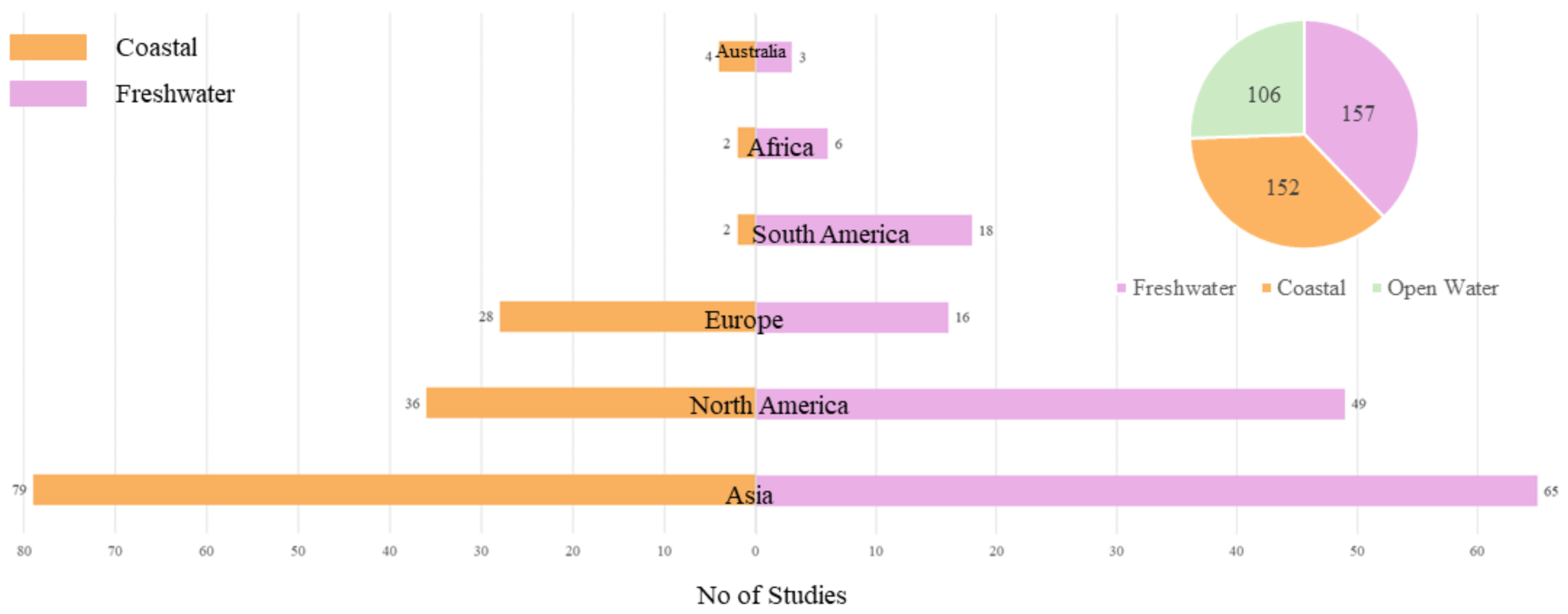
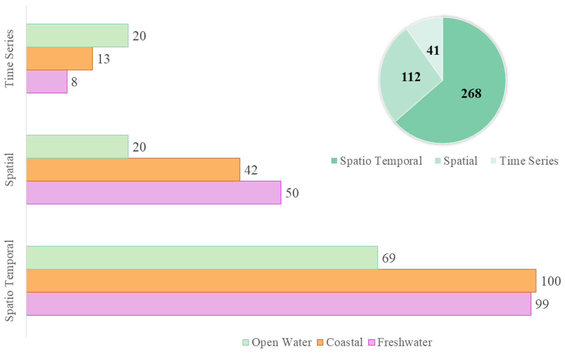
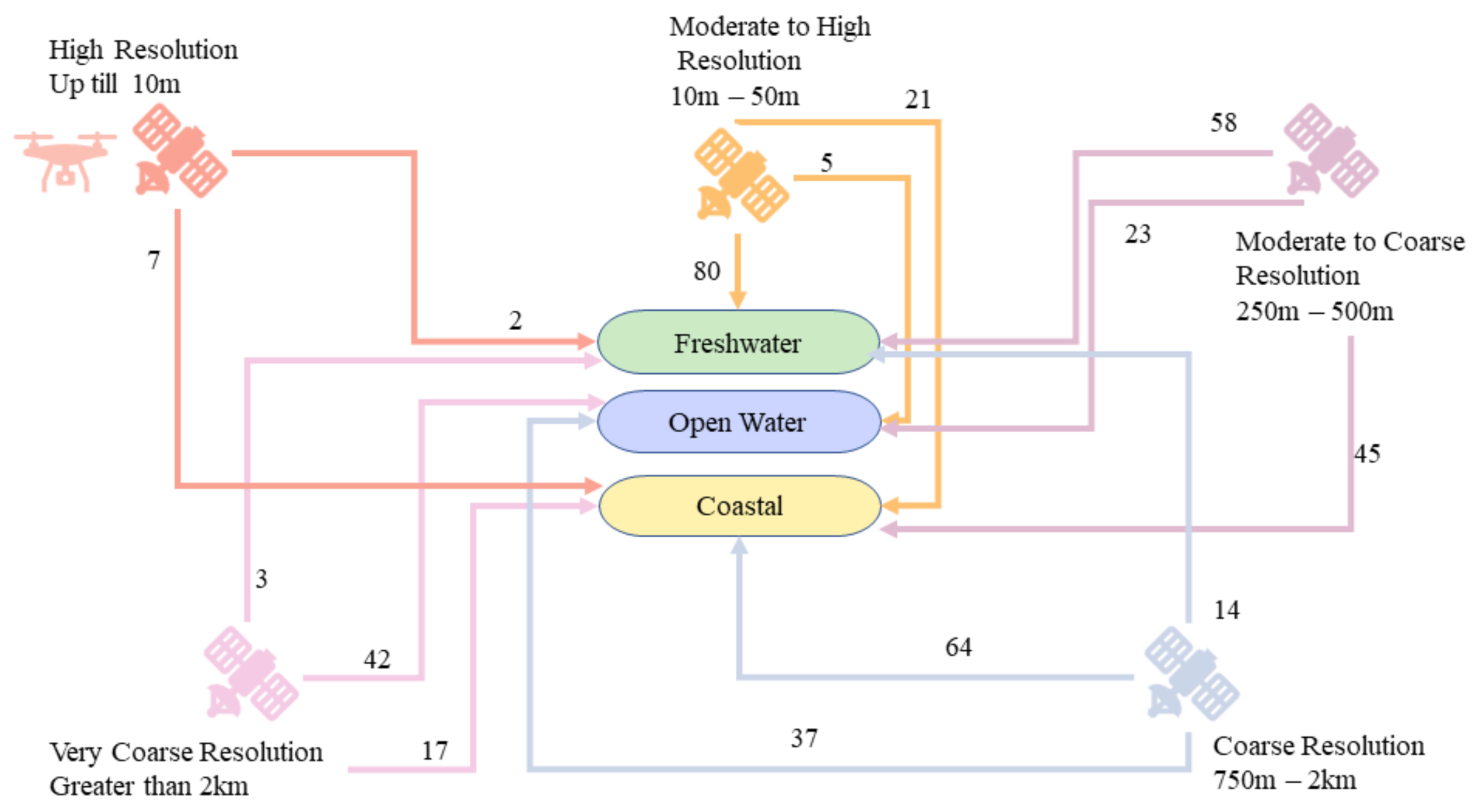
| A (Parameter Studied) | B (Data Set Used) | C (Methodology/Analysis) |
|---|---|---|
| “Algal bloom” | “satellite Imag*” | Detect* |
| OR Cyanobacteria* | OR “Satellite data” | OR Monitor* |
| OR Phytoplankton | OR MODIS | OR Map* |
| OR “Red Tide” | OR MERIS | OR Observ* |
| OR “Green Tide” | OR landsat | OR Model* |
| OR “Phycocyanin” | OR SeaWiFS | OR Compar* |
| OR “Chlorophyll-a” | OR Sentinel | OR Estimat* |
| OR “Macro alga*” | OR Satellite | OR Retriev* |
| OR “Spring bloom” | OR “Earth Observation” | OR Evaluat* |
| OR “Winter bloom” | OR GOCI | OR Application |
| OR “Summer bloom” | OR UAV | OR Algorithm |
| OR “HAB” | OR SAR | OR Assess* |
| OR Analy* | ||
| OR Determin* | ||
| OR Spati* | ||
| OR Temporal | ||
| OR Variat* | ||
| OR Classif* | ||
| OR Deriv* |
| No. | Author [Reference] | Year | Journal | Impact Factor | Citations Total |
|---|---|---|---|---|---|
| 1 | Pahlevan [52] | 2020 | Remote Sensing of Environment | 10.164 | 71 |
| 2 | Kuhn [122] | 2019 | Remote Sensing of Environment | 10.164 | 91 |
| 3 | Tomlinson [123] | 2016 | Remote Sensing Letters | 2.298 | 173 |
| 4 | Hu [51] | 2010 | Journal of Geophysical Research | 2.799 | 307 |
| 5 | Siegel [94] | 2013 | Remote Sensing of Environment | 10.164 | 222 |
| 6 | Kahru [124] | 2014 | Biogeosciences | 3.48 | 173 |
| 7 | Hu [61] | 2005 | Remote Sensing of Environment | 10.164 | 386 |
| 8 | Shi [125] | 2017 | Scientific Reports—Nature | 4.379 | 96 |
| 9 | Soria-Perpinya [126] | 2020 | Science of the Total Environment | 7.963 | 23 |
| 10 | Binding [100] | 2018 | Journal of Great Lakes Research | 2.48 | 69 |
| Satellite | Sensor | No. of Studies (Single Sensor) | No. of Studies (in Combination) | Frequent Sensors Used in Combination |
|---|---|---|---|---|
| Landsat 5 | TM | 10 | 18 | ETM+, OLI |
| Landsat 7 | ETM+ | 10 | 19 | TM, OLI, MSI |
| Landsat 8 | OLI | 25 | 26 | TM, ETM+, MSI, OLCI |
| Sentinel 2 | MSI | 12 | 20 | ETM+, OLI, OLCI |
| Sentinel 3 | OLCI | 6 | 12 | OLI, MSI |
| Aqua/Terra | MODIS | 103 | 59 | MERIS, SeaWiFS, TM, ETM+, OLI, MSI, OLCI |
| Envisat | MERIS | 49 | 32 | MODIS, SeaWIFS, OLCI |
| Orbview-2 | SeaWiFS | 56 | 37 | MODIS, MERIS |
| Ancillary Data Category | Detail |
|---|---|
| Water quality parameters | Total suspended matter (TSM), turbidity, Secchi disk depth (SDD), colored dissolved organic matter (CDOM), total nitrogen (TN), total phosphorus (TP), dissolved oxygen (DO), salinity |
| Sea surface parameters | Sea surface height (SSH), sea surface temperature (SST), sea surface height anomaly (SSHA), mixed layer depth (MLD) |
| Wind parameters | Wind speed, wind vectors, wind stress, wind mixing |
| Other meteorological data | Rainfall, temperature, cloud cover |
| Radiation parameters | Photosynthetically active radiation (PAR), solar flux, diffused attenuation coefficient, normalized water-leaving radiance |
| Hydrological data | River and storm water runoff |
| Ocean and bathymetric data | North Atlantic oscillation index, bathymetric maps, geostrophic current |
Publisher’s Note: MDPI stays neutral with regard to jurisdictional claims in published maps and institutional affiliations. |
© 2021 by the authors. Licensee MDPI, Basel, Switzerland. This article is an open access article distributed under the terms and conditions of the Creative Commons Attribution (CC BY) license (https://creativecommons.org/licenses/by/4.0/).
Share and Cite
Khan, R.M.; Salehi, B.; Mahdianpari, M.; Mohammadimanesh, F.; Mountrakis, G.; Quackenbush, L.J. A Meta-Analysis on Harmful Algal Bloom (HAB) Detection and Monitoring: A Remote Sensing Perspective. Remote Sens. 2021, 13, 4347. https://doi.org/10.3390/rs13214347
Khan RM, Salehi B, Mahdianpari M, Mohammadimanesh F, Mountrakis G, Quackenbush LJ. A Meta-Analysis on Harmful Algal Bloom (HAB) Detection and Monitoring: A Remote Sensing Perspective. Remote Sensing. 2021; 13(21):4347. https://doi.org/10.3390/rs13214347
Chicago/Turabian StyleKhan, Rabia Munsaf, Bahram Salehi, Masoud Mahdianpari, Fariba Mohammadimanesh, Giorgos Mountrakis, and Lindi J. Quackenbush. 2021. "A Meta-Analysis on Harmful Algal Bloom (HAB) Detection and Monitoring: A Remote Sensing Perspective" Remote Sensing 13, no. 21: 4347. https://doi.org/10.3390/rs13214347
APA StyleKhan, R. M., Salehi, B., Mahdianpari, M., Mohammadimanesh, F., Mountrakis, G., & Quackenbush, L. J. (2021). A Meta-Analysis on Harmful Algal Bloom (HAB) Detection and Monitoring: A Remote Sensing Perspective. Remote Sensing, 13(21), 4347. https://doi.org/10.3390/rs13214347