
A Novel Noise Reduction Method of UAV Magnetic Survey Data Based on CEEMDAN, Permutation Entropy, Correlation Coefficient and Wavelet Threshold Denoising


Abstract
:1. Introduction
- 1.
- The adaptive decomposition algorithm, i.e., CEEMDAN, is applied to multi-rotor UAV magnetic data for the first time. The original data are decomposed into a set of IMF components with different scales.
- 2.
- The IMFs are divided into four categories, i.e., noise IMFs, noise-dominant IMFs, signal-dominant IMFs, and signal IMFs according to the quartiles of PE, which is completely determined by the characteristics of the signal itself without setting a threshold artificially.
- 3.
- The real signal-dominant IMFs are identified using CC, while the wavelet soft threshold denoising (WSTD) is applied to further suppress noise. Simulation results show that the signal-to-noise ratio (SNR) of the signal can be improved by about 16–20 dB after denoising by means of the proposed method.
2. Relevant Principles
2.1. Principles of EMD, EEMD, and CEEMDAN Algorithm
2.1.1. EMD Algorithm
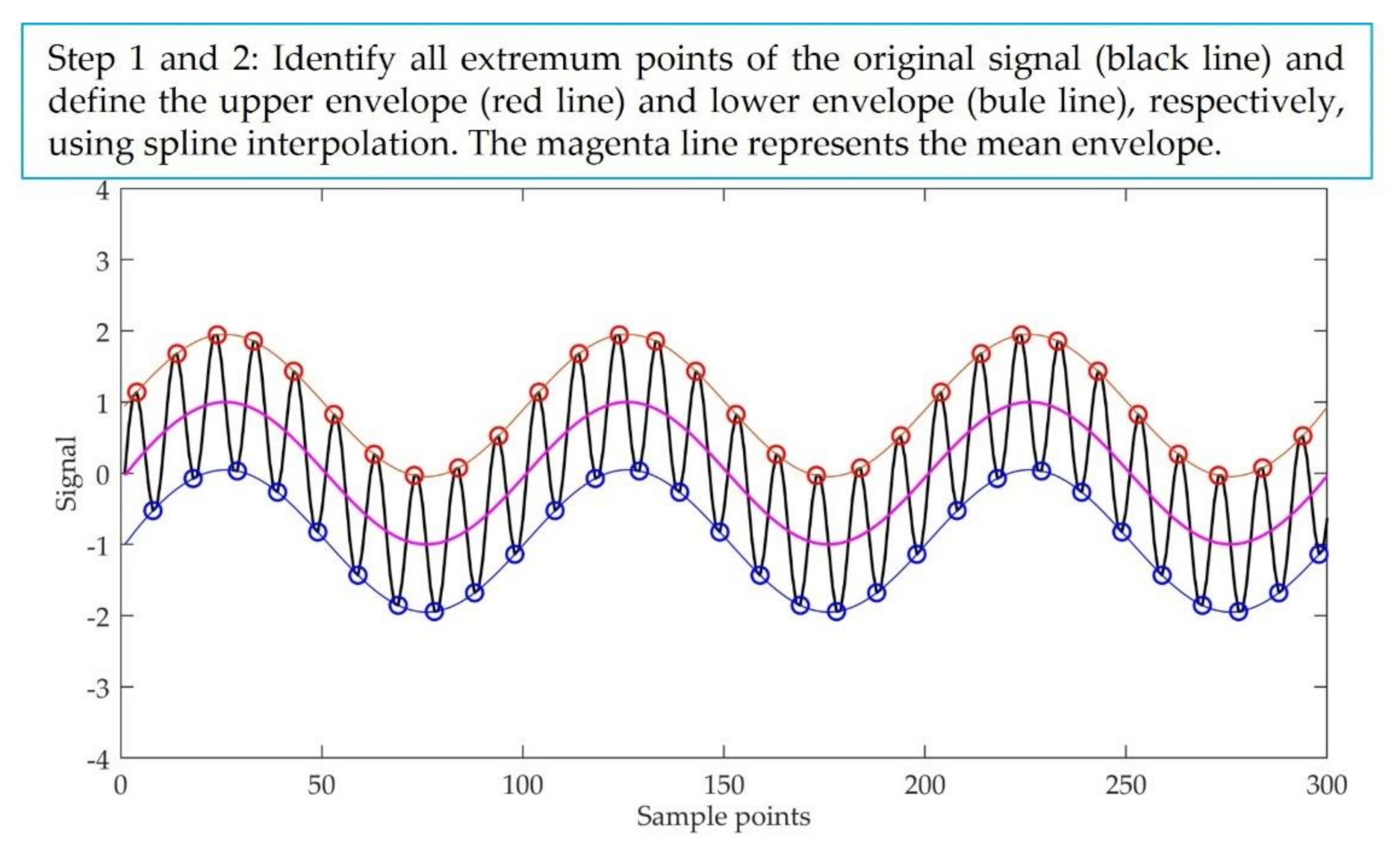
- Step 1:
- Identify all the extremum points of the original signal and define the upper and lower envelope and , respectively, using a cubic spline interpolation.
- Step 2:
- Calculate the mean envelope of the upper and lower envelope.
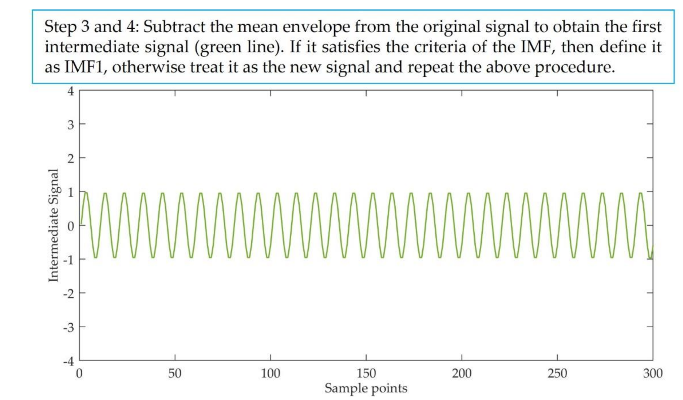
- Step 3:
- Subtract the mean envelope from s(t) to obtain the first intermediate signal.
- Step 4:
- If satisfies the criteria of the IMF, then define , otherwise treat as the new signal and repeat the above procedure k times until satisfies the IMF conditions. The acquisition of IMF usually requires several iterations. To finish the iteration, the stopping criterion is defined as follows:where n is the length of the intermediate signal. The iteration will be stopped when (in this study is set to 0.3).
- Step 5:
- Let , treat as the new signal and repeat Step 1–4 to obtain the next IMF, until becomes either a constant or a monotonic function. Finally, the original signal s(t) after EMD can be expressed as:where N is the number of IMFs, and is the final residue.
| Algorithm 1: EMD |
| Input: The original signal . |
| Output: Several IMF and a residue, i.e., and . |
| 1: function EMD (, , ) |
| 2: IMF0 |
| 3: i0 |
| 4: N |
| 5: residue |
| 6: while residue> do |
| 7: ii+1 |
| 8: |
| 9: |
| 10: while do |
| 11: for j = 1j = N do |
| 12: [, ] |
| 13: [, ] |
| 14: end for |
| 15: |
| 16: |
| 17: |
| 18: |
| 19: |
| 20: end while |
| 21: |
| 22: residue |
| 23: end while |
| 24: return IMF and residue |
| 25: end function |
2.1.2. EEMD Algorithm
- Step 1:
- Different Gaussian white noise signals with zero mean and unit variance are added to the original signal to obtain a set of new signals
- Step 2:
- Decompose each by EMD to obtain , where denotes the number of IMFs.
- Step 3:
- Average the to obtain the EEMD mode
| Algorithm 2: EEMD |
| Input: The original signal , the amplitude of the added Gaussian noise , and the number of ensemble trials . |
| Output: Several IMF and a residue, i.e., and . |
| 1: function EEMD (, , ) |
| 2: IMF0 |
| 3: r |
| 4: for i = 1 = do |
| 5: |
| 6: |
| 7: EMD () |
| 8: |
| 9: end for |
| 10: for k = 1 = p do |
| 11: ) |
| 12: end for |
| 13: |
| 14: return IMF and residue |
| 15: end function |
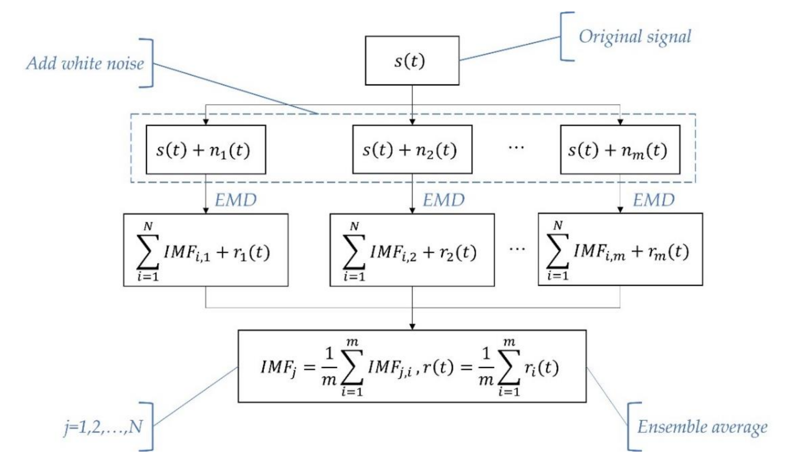
2.1.3. CEEMDAN Algorithm
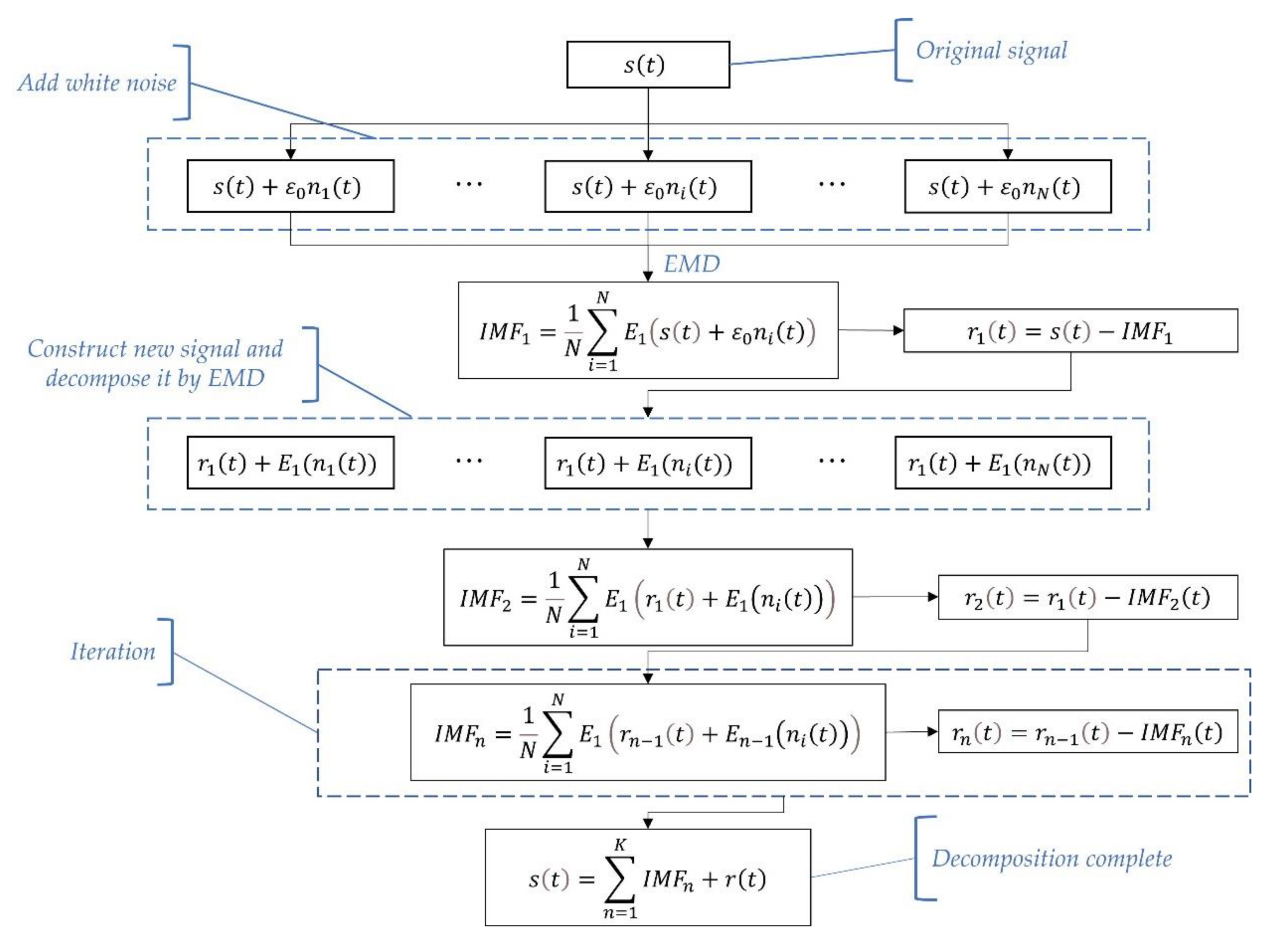
- Step 1:
- The white noise is added to the original signal , and the first IMF of CEEMDAN is obtained by calculating the ensemble average:where is defined as the nth mode component of EMD.
- Step 2:
- The first residual component can be obtained
- Step 3:
- Construct the new signaland decompose it by EMD. The second mode component can be obtained:
- Step 4:
- The nth residual signal and the (n+1)th IMF can be obtained according to the process of Step 3
- Step 5:
- Repeat Step 4 until the residual signal is no longer decomposed. The original signal can be expressed aswhere K is the number of IMFs by CEEMDAN, and is the final residual mode.
| Algorithm 3: CEEMDAN |
| Input: The original signal , the amplitude of the added Gaussian noise , and the number of ensemble trials . |
| Output: Several IMF and a residue, i.e., and . |
| 1: function CEEMDAN (, , ) |
| 2: IMF0 |
| 3: residue |
| 4: for i = 1 = do |
| 5: |
| 6: |
| 7: () |
| 8: |
| 9: end for |
| 10: |
| 11: for k = 2 = p do |
| 12: |
| 13: |
| 14: end for |
| 15: |
| 16: return IMF and residue |
| 17: end function |
| 18: |
| 19: function () |
| 20: EMD () |
| 21: |
| 22: return |
| 23: end function |
2.2. Permutation Entropy
- Step 1:
- The first step in the calculation of permutation entropy requires extracting ordinal information from the time series. Given a time series , K reconstructed time series can be obtained as:where and represent the embedding dimension and time delay, respectively. .
- Step 2:
- For the jth reconstructed component, rearrange it in ascending order:
- Step 3:
- The permutation of (15) is defined as:
- Step 4:
- If the probabilities of each permutation are , respectively. The PE of time series is defined as
- Step 5:
- PE can be normalized as
| Algorithm 4: PE [34] |
| Input: The time series , the embedding dimension . |
| Output: PE (, ). |
| Define: is the k-th permutation of , time delay = 1. |
| 1: function PE (, ) |
| 2: PE0 |
| 3: Nlength () |
| 4: |
| 5: |
| 6: |
| 7: |
| 8: for j = 0= N do |
| 9: |
| 10: |
| 11: for i = 0 = do |
| 12: if then |
| 13: |
| 14: break |
| 15: end for |
| 16: end for |
| 17: for k = 0 = do |
| 18: |
| 19: if then |
| 20: |
| 21: end if |
| 22: end for |
| 23: return PE |
| 24: end function |
2.3. Correlation Coefficient
2.4. Wavelet Threshold Denoising
- Step 1:
- Proper wavelet basis function and decomposition level are selected to conduct wavelet decomposition on the noisy signal .
- Step 2:
- The thresholds are estimated according to appropriate threshold selection criteria for the high-frequency coefficients at different decomposition scales.
- Step 3:
- The low-frequency coefficients of decomposition and the threshold high-frequency coefficients are used to reconstruct signals.
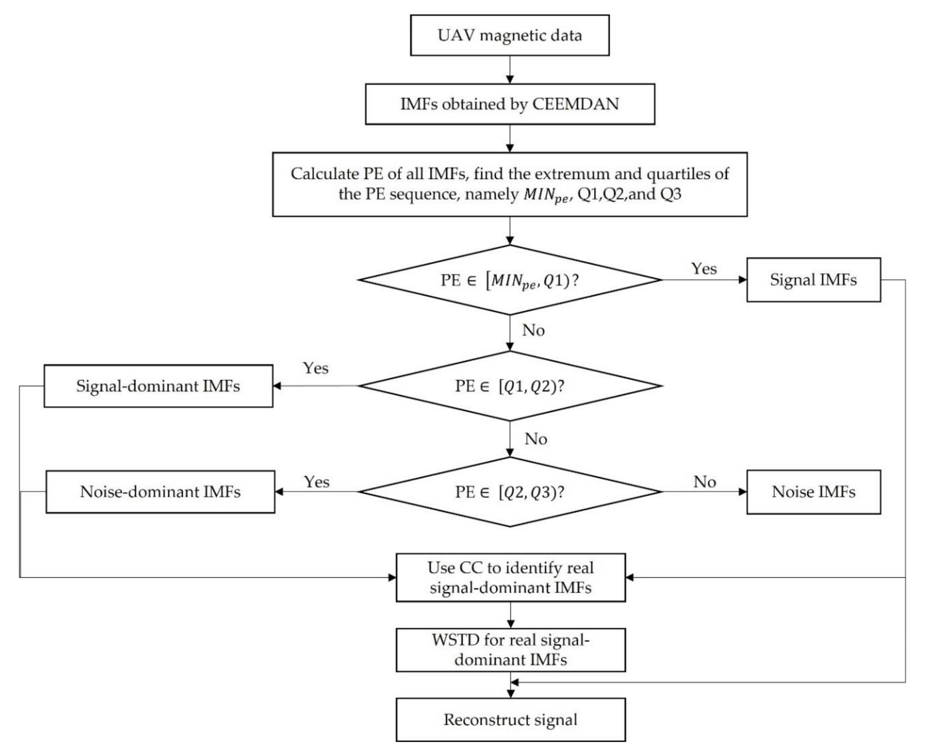
3. The Proposed Method for UAV Magnetic Data Denoising
- Step 1:
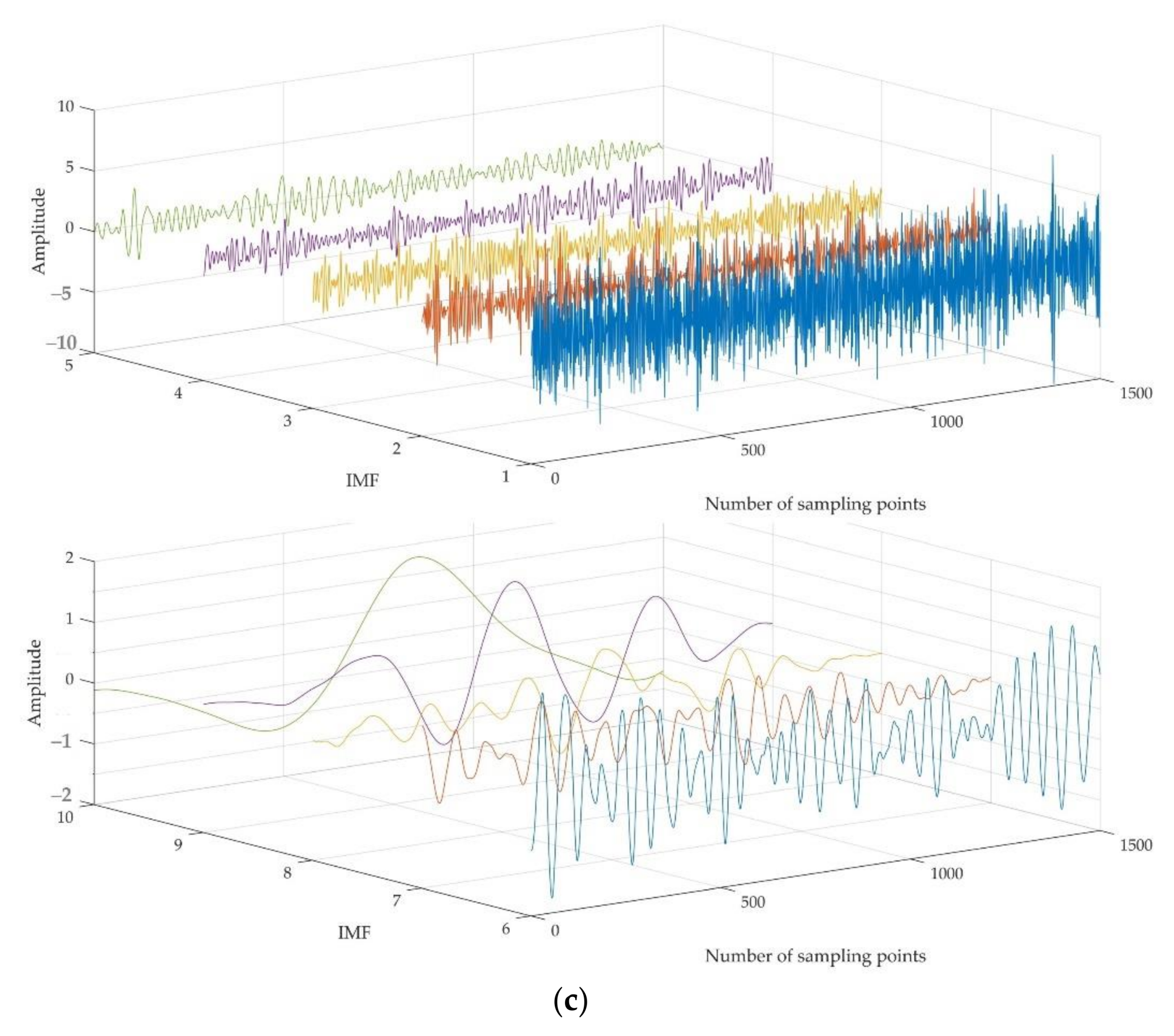
- The original signal is decomposed into several IMFs by CEEMDAN and arranged from high frequency to low frequency.
- Step 2:
- Calculate the PE of all IMFs, the PE sequence is arranged in ascending order, and the extremum and the quartiles of the PE sequence are found, namely , Q1, Q2, Q3, and .
- Step 3:
- Execute the judgement procedure: (1) if PE falls in the interval of , the corresponding IMFs are considered as signal IMFs and are preserved; (2) if PE falls in the interval of , the corresponding IMFs are defined as signal-dominant IMFs; (3) if PE falls in the interval of , the corresponding IMFs are defined as noise-dominant IMFs; (4) if PE falls in the interval of , the corresponding IMFs are defined as noise and are removed.
- Step 4:
- The CCs between signal (noise)-dominant IMFs and the real signal which is constituted by signal IMFs are obtained. The median of the absolute value sequence of CCs is recorded as , and the IMFs corresponding to the CC greater than are defined as the real signal-dominant IMFs.
- Step 5:
- WSTD is applied to the real signal-dominant IMFs. The wavelet basis function and the decomposition level are db4 and 4, respectively.
- Step 6:
- The denoised signal can be obtained by combining the signal IMFs and the denoised IMFs.
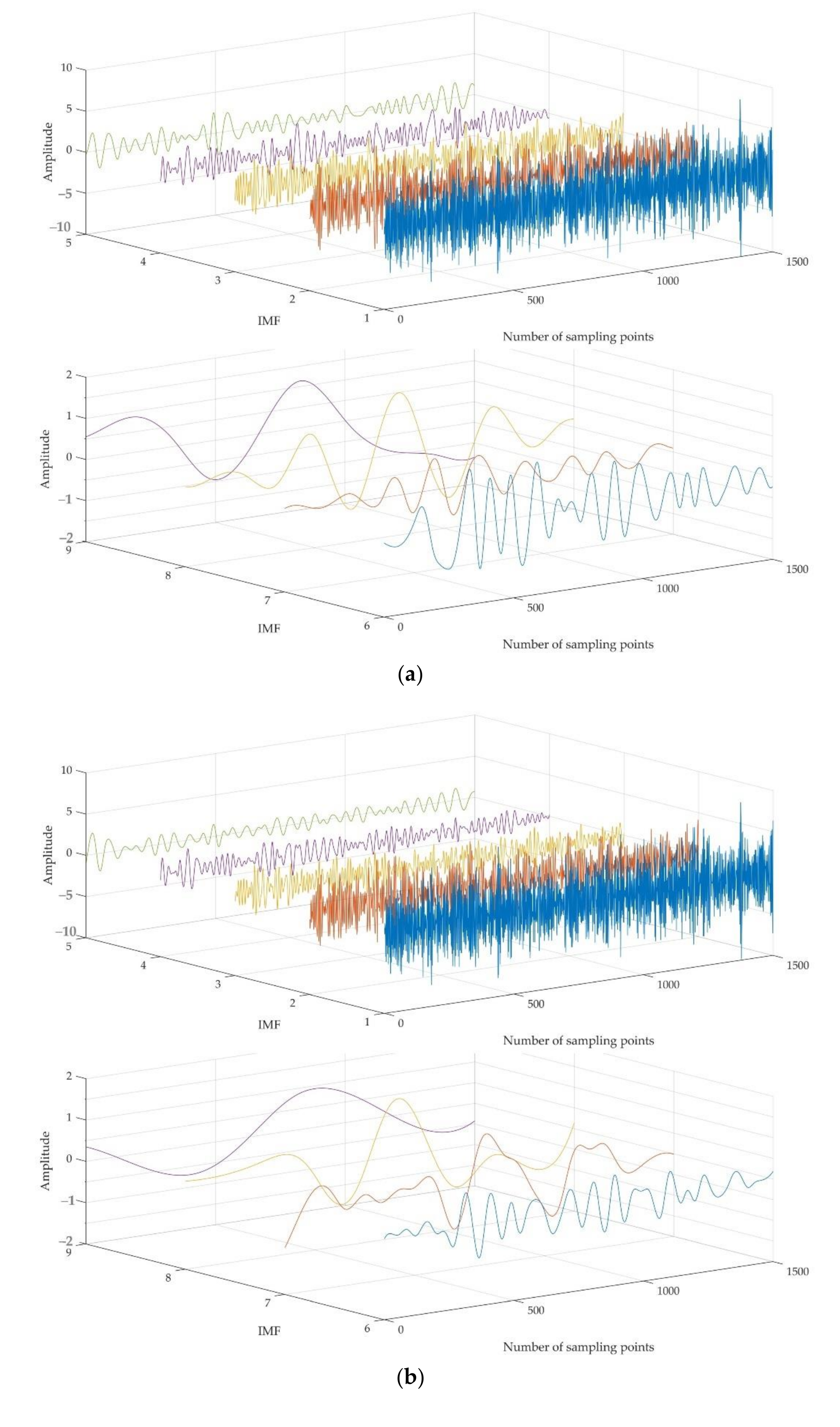
4. Synthetic Signal Denoising Experiment
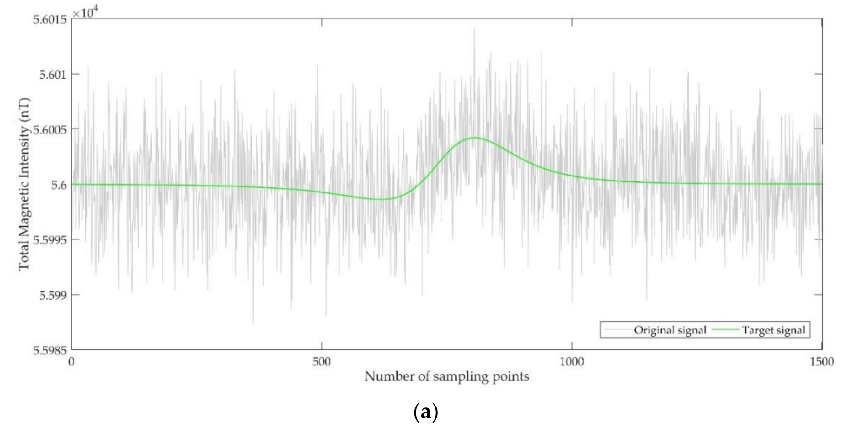
4.1. Acquisition of Synthetic Signal
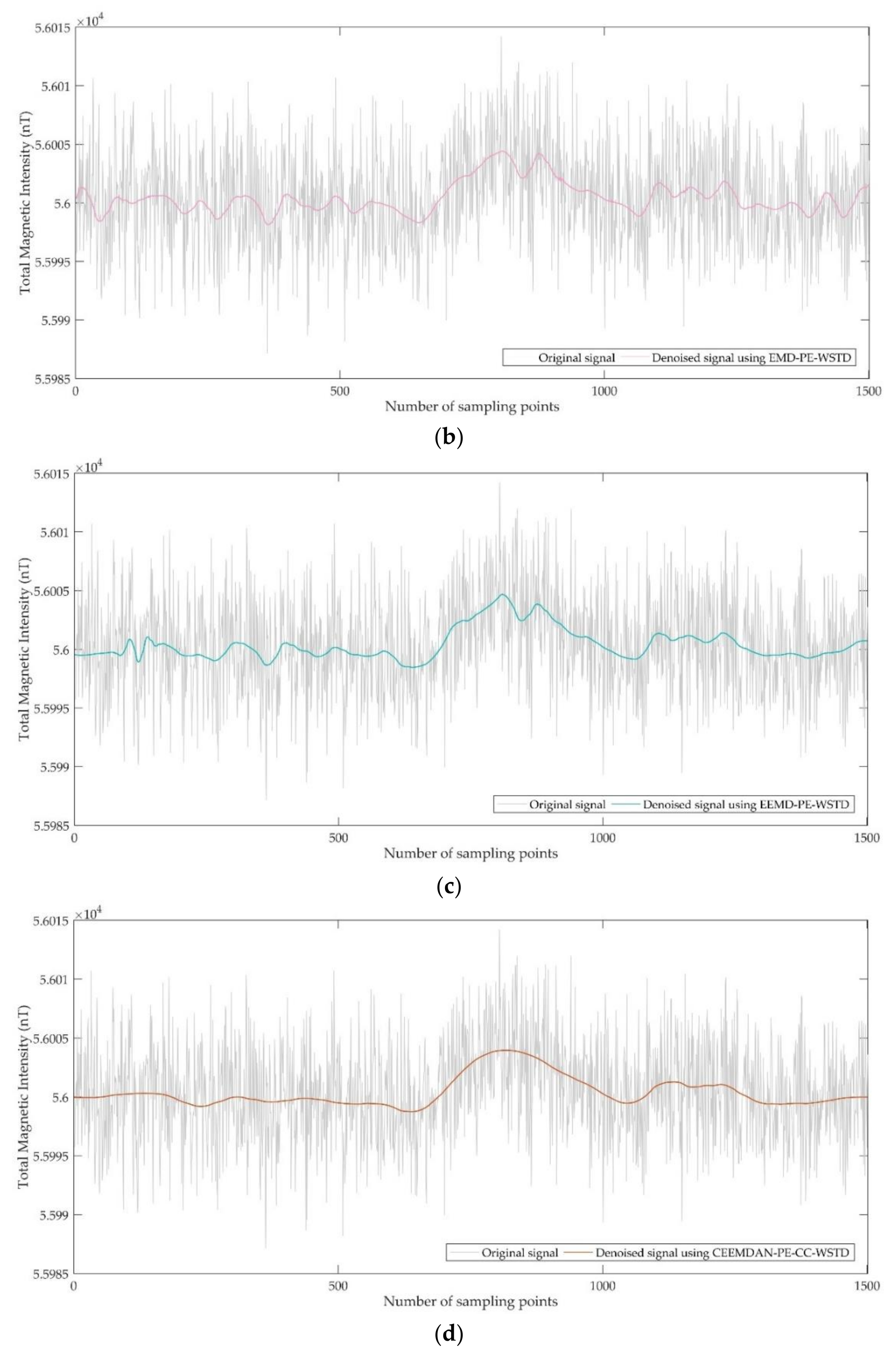
4.2. Evaluation of Different Denoising Methods
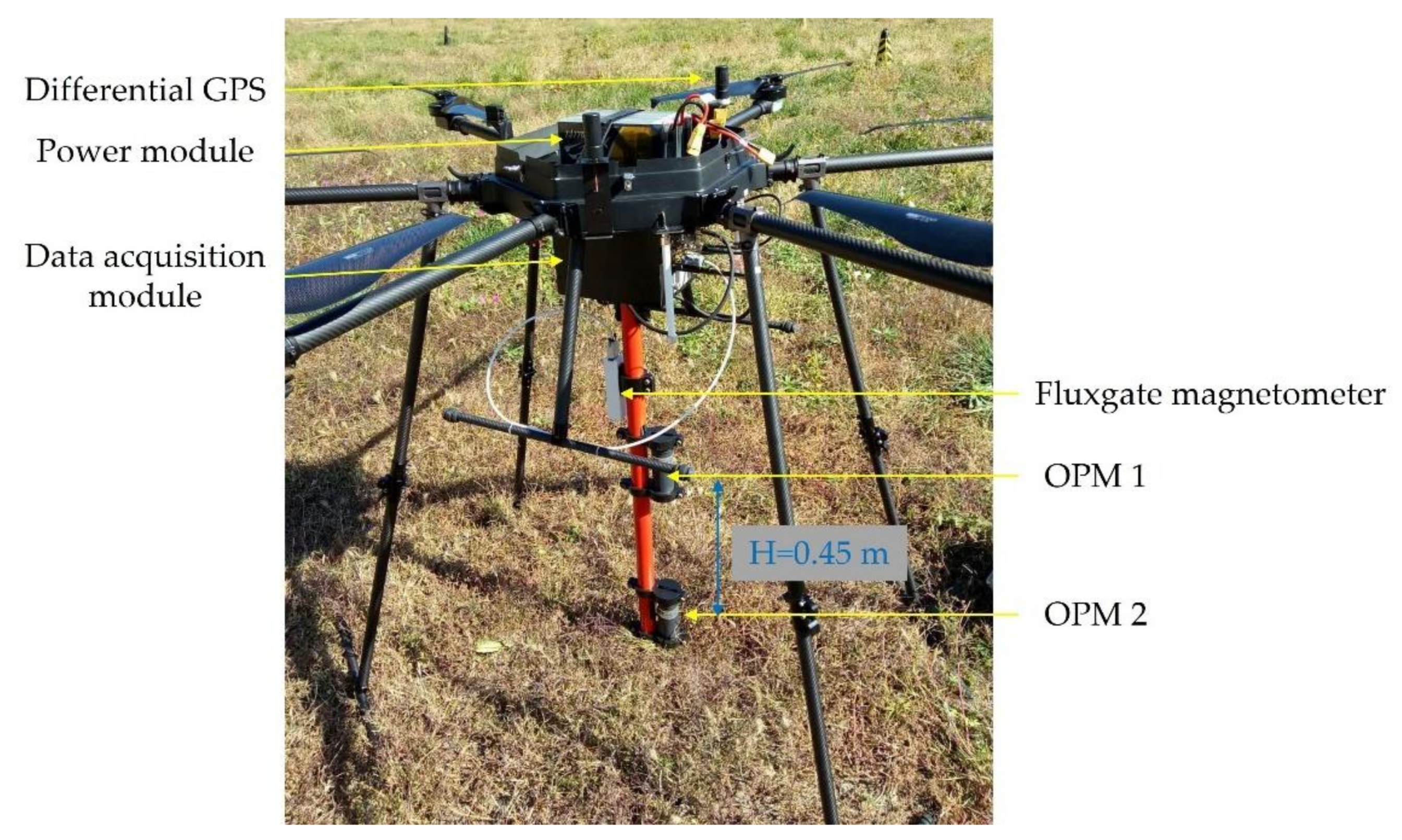
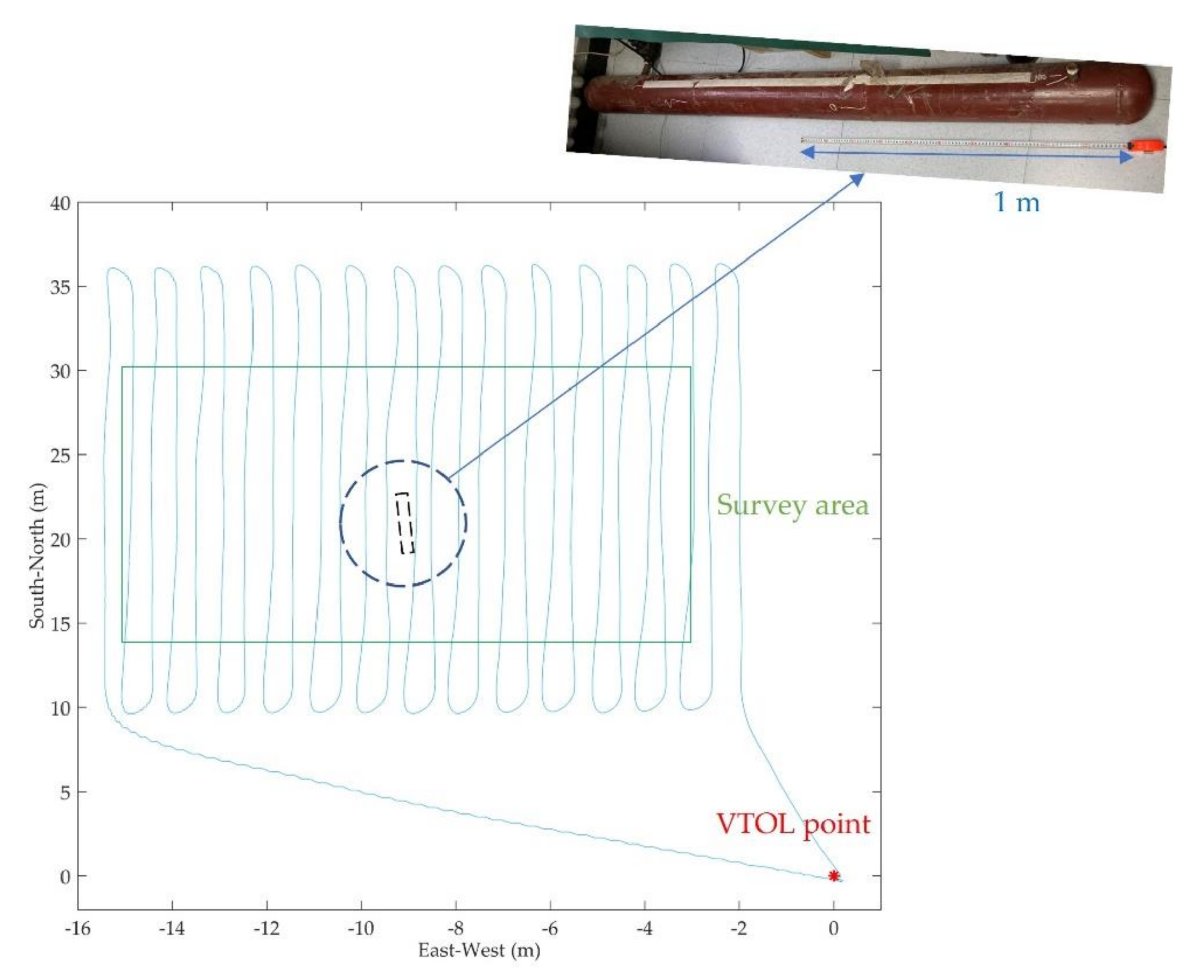
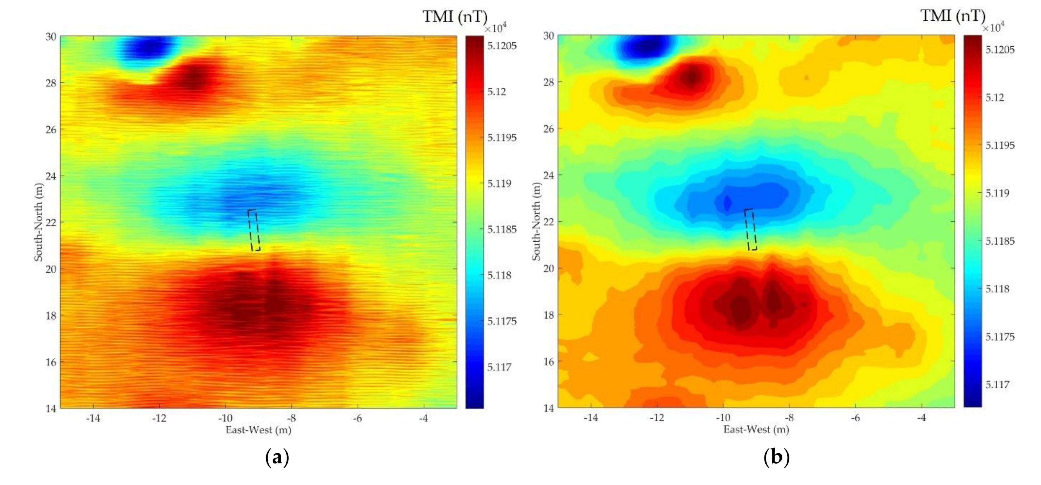
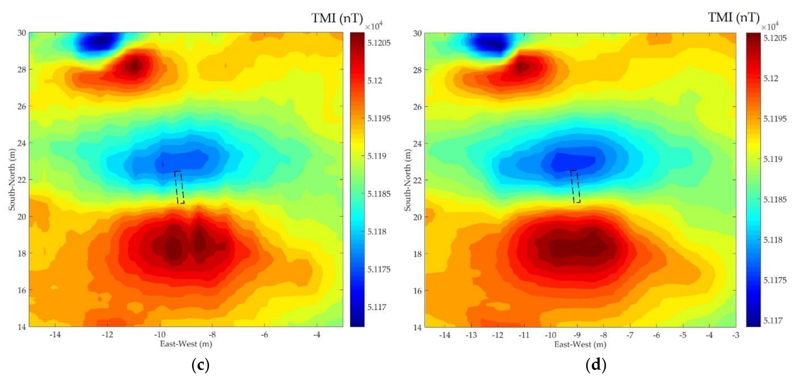
5. UAV Magnetic Survey Experiment Verification
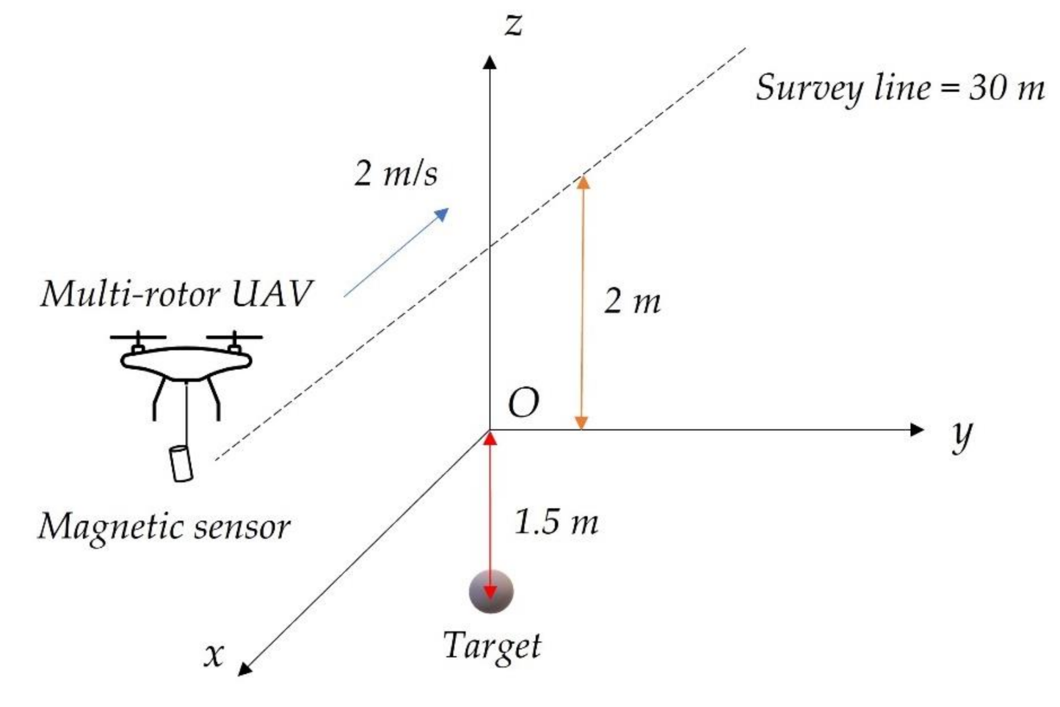
5.1. The Multi-Rotor UAV Magnetic Survey System
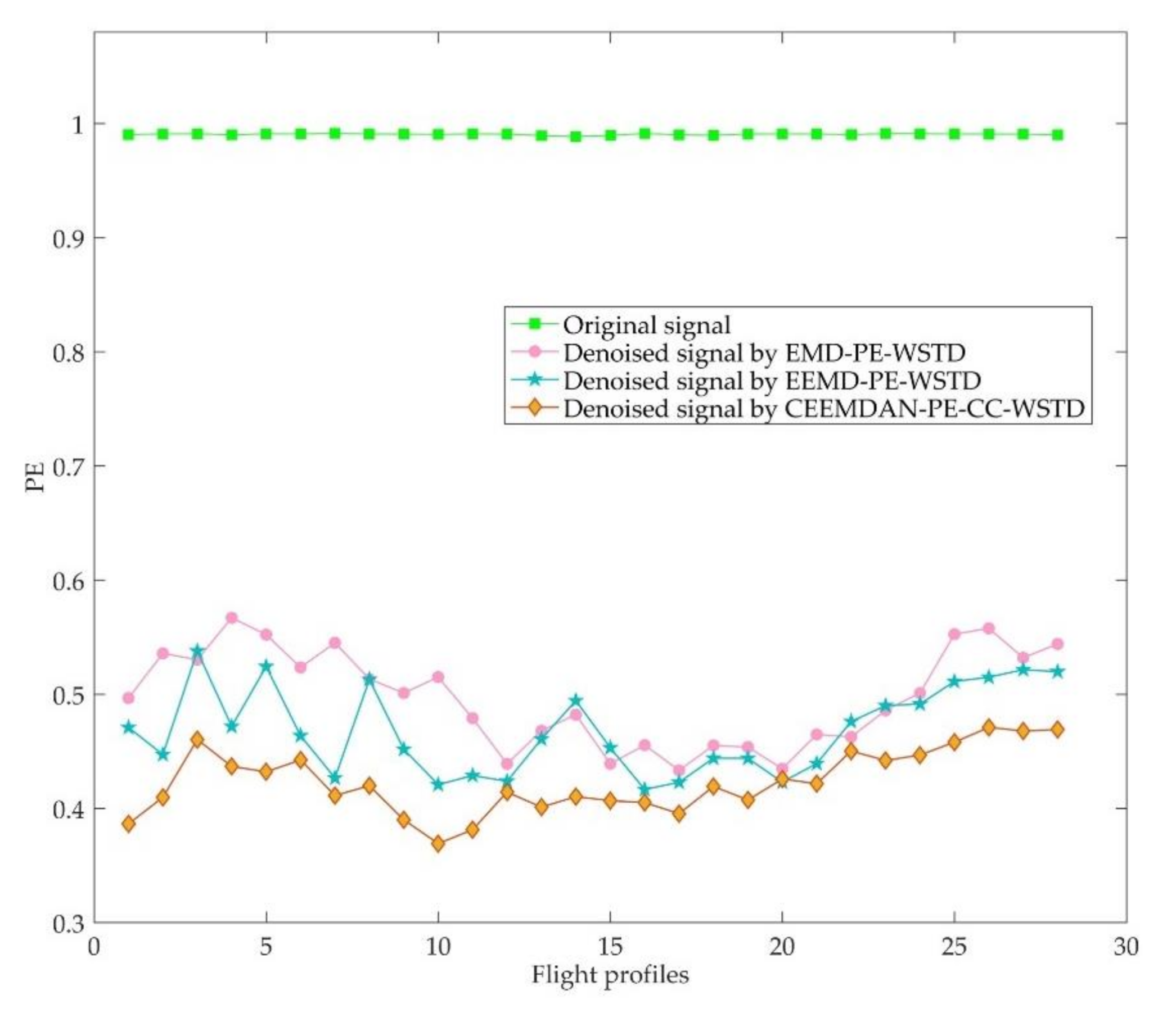
5.2. Evaluation of UAV-Borne Magnetic Survey Results after Denoising
6. Conclusions
Author Contributions
Funding
Institutional Review Board Statement
Informed Consent Statement
Data Availability Statement
Acknowledgments
Conflicts of Interest
Abbreviations
| AGL | Above ground level |
| CC | Correlation coefficient |
| CEEMDAN | Complete ensemble empirical mode decomposition with adaptive noise |
| EEMD | Ensemble empirical mode decomposition |
| EMD | Empirical mode decomposition |
| IGRF | International Geomagnetic Reference Field |
| IMF | Intrinsic mode function |
| OPMs | Optically pumped magnetometers |
| PE | Permutation entropy |
| PSNR | Peak signal-to-noise ratio |
| RMSE | Root mean square error |
| SNR | Signal-to-noise ratio |
| SSIM | Structural similarity |
| TMI | Total magnetic intensity |
| UAV | Unmanned aerial vehicle |
| UXO | Unexploded ordnance |
| VMI | Vector magnetic intensity |
| VTOL | Vertical take-off and landing |
| WSTD | Wavelet soft threshold denoising |
References
- Zheng, Y.; Li, S.; Xing, K.; Zhang, X. Unmanned Aerial Vehicles for Magnetic Surveys: A Review on Platform Selection and Interference Suppression. Drones 2021, 5, 93. [Google Scholar] [CrossRef]
- Vadim, T.; Alexander, P.; Vasily, A.; Dmitry, K. Unmanned airborne magnetic survey technologies: Present and future. In Recent Advances in Rock Magnetism, Environmental Magnetism and Paleomagnetism; Springer International Publishing: Cham, Switzerland, 2019; pp. 523–534. [Google Scholar]
- Døssing, A.; Silva, E.L.S.D.; Martelet, G.; Rasmussen, T.M.; Gloaguen, E.; Petersen, J.T.; Linde, J. A high-speed, light-weight scalar magnetometer bird for km scale UAV magnetic surveying: On sensor choice, bird design, and quality of output data. Remote Sens. 2021, 13, 649. [Google Scholar] [CrossRef]
- Hashimoto, T.; Koyama, T.; Kaneko, T.; Ohminato, T.; Yanagisawa, T.; Yoshimoto, M.; Suzuki, E. Aeromagnetic survey using an unmanned autonomous helicopter over Tarumae Volcano, northern Japan. Explor. Geophys. 2014, 45, 37–42. [Google Scholar] [CrossRef] [Green Version]
- Gailler, L.; Labazuy, P.; Régis, E.; Bontemps, M.; Souriot, T.; Bacques, G.; Carton, B. Validation of a new UAV magnetic prospecting tool for volcano monitoring and geohazard assessment. Remote Sens. 2021, 13, 894. [Google Scholar] [CrossRef]
- Malehmir, A.; Dynesius, L.; Paulusson, K.; Paulusson, A.; Johansson, H.; Bastani, M.; Wedmark, M.; Marsden, P. The potential of rotary-wing UAV-based magnetic surveys for mineral exploration: A case study from central Sweden. Lead. Edge 2017, 36, 552–557. [Google Scholar] [CrossRef]
- Walter, C.; Braun, A.; Fotopoulos, G. Spectral analysis of magnetometer swing in high-resolution UAV-borne aeromagnetic surveys. In Proceedings of the 2019 IEEE Systems and Technologies for Remote Sensing Applications Through Unmanned Aerial Systems (STRATUS), Rochester, NY, USA, 25–27 February 2019; pp. 1–4. [Google Scholar]
- Mu, Y.; Zhang, X.; Xie, W.; Zheng, Y. Automatic detection of near-surface targets for unmanned aerial vehicle (UAV) magnetic survey. Remote Sens. 2020, 12, 452. [Google Scholar] [CrossRef] [Green Version]
- Schmidt, V.; Becken, M.; Schmalzl, J. A UAV-borne magnetic survey for archaeological prospection of a Celtic burial site. First Break 2020, 38, 61–66. [Google Scholar] [CrossRef]
- Shahsavani, H. An aeromagnetic survey carried out using a rotary-wing UAV equipped with a low-cost magneto-inductive sensor. Int. J. Remote Sens. 2021, 1–14. [Google Scholar] [CrossRef]
- Liu, D.; Xu, X.; Huang, C.; Zhu, W.; Liu, X.; Yu, G.; Fang, G. Adaptive cancellation of geomagnetic background noise for magnetic anomaly detection using coherence. Meas. Sci. Technol. 2014, 26, 015008. [Google Scholar] [CrossRef]
- Wang, S.; Wang, J. Application of Higher-Order Statistics in Magnetotelluric Data Processing. Chin. J. Geophys. 2004, 47, 1046–1053. [Google Scholar] [CrossRef]
- Huang, N.E.; Shen, Z.; Long, S.R.; Wu, M.C.; Shih, H.H.; Zheng, Q.; Yen, N.-C.; Tung, C.C.; Liu, H.H. The empirical mode decomposition and the Hilbert spectrum for nonlinear and non-stationary time series analysis. Proc. R. Soc. Lond. Ser. A Math. Phys. Eng. Sci. 1998, 454, 903–995. [Google Scholar] [CrossRef]
- Campolo, M.; Labate, D.; La Foresta, F.; Morabito, F.C.; Lay-Ekuakille, A.; Vergallo, P. ECG-derived respiratory signal using empirical mode decomposition. In Proceedings of the 2011 IEEE International Symposium on Medical Measurements and Applications, Bari, Italy, 30–31 May 2011; pp. 399–403. [Google Scholar]
- Wu, Z.; Huang, N.E. Ensemble empirical mode decomposition: A noise-assisted data analysis method. Adv. Adapt. Data Anal. 2009, 1, 1–41. [Google Scholar] [CrossRef]
- Torres, M.E.; Colominas, M.A.; Schlotthauer, G.; Flandrin, P. A complete ensemble empirical mode decomposition with adaptive noise. In Proceedings of the 2011 IEEE international conference on acoustics, speech and signal processing (ICASSP), Prague, Czech Republic, 22–27 May 2011; pp. 4144–4147. [Google Scholar]
- Xu, Y.; Luo, M.; Li, T.; Song, G. ECG signal de-noising and baseline wander correction based on CEEMDAN and wavelet threshold. Sensors 2017, 17, 2754. [Google Scholar] [CrossRef] [PubMed] [Green Version]
- Yao, L.; Pan, Z. A new method based CEEMDAN for removal of baseline wander and powerline interference in ECG signals. Optik 2020, 223, 165566. [Google Scholar] [CrossRef]
- Zhang, W.; Qu, Z.; Zhang, K.; Mao, W.; Ma, Y.; Fan, X. A combined model based on CEEMDAN and modified flower pollination algorithm for wind speed forecasting. Energy Conv. Manag. 2017, 136, 439–451. [Google Scholar] [CrossRef]
- Liang, T.; Xie, G.; Fan, S.; Meng, Z. A Combined Model Based on CEEMDAN, Permutation Entropy, Gated Recurrent Unit Network, and an Improved Bat Algorithm for Wind Speed Forecasting. IEEE Access 2020, 8, 165612–165630. [Google Scholar] [CrossRef]
- Cao, J.; Li, Z.; Li, J. Financial time series forecasting model based on CEEMDAN and LSTM. Phys. A Stat. Mech. Appl. 2019, 519, 127–139. [Google Scholar] [CrossRef]
- Bai, L.; Han, Z.; Li, Y.; Ning, S. A hybrid de-noising algorithm for the gear transmission system based on CEEMDAN-PE-TFPF. Entropy 2018, 20, 361. [Google Scholar] [CrossRef] [Green Version]
- Kuai, M.; Cheng, G.; Pang, Y.; Li, Y. Research of planetary gear fault diagnosis based on permutation entropy of CEEMDAN and ANFIS. Sensors 2018, 18, 782. [Google Scholar] [CrossRef] [Green Version]
- Jiang, L.; Tan, H.; Li, X.; Chen, L.; Yang, D. CEEMDAN-based permutation entropy: A suitable feature for the fault identification of spiral-bevel gears. Shock Vib. 2019, 1, 1–13. [Google Scholar] [CrossRef]
- Li, Y.; Li, Y.; Chen, X.; Yu, J.; Yang, H.; Wang, L. A new underwater acoustic signal denoising technique based on CEEMDAN, mutual information, permutation entropy, and wavelet threshold denoising. Entropy 2018, 20, 563. [Google Scholar] [CrossRef] [Green Version]
- Li, G.; Guan, Q.; Yang, H. Noise reduction method of underwater acoustic signals based on CEEMDAN, effort-to-compress complexity, refined composite multiscale dispersion entropy and wavelet threshold denoising. Entropy 2019, 21, 11. [Google Scholar] [CrossRef] [Green Version]
- Mousavi, A.A.; Zhang, C.; Masri, S.F.; Gholipour, G. Structural damage localization and quantification based on a CEEMDAN Hilbert transform neural network approach: A model steel truss bridge case study. Sensors 2020, 20, 1271. [Google Scholar] [CrossRef] [PubMed] [Green Version]
- Li, X.; Li, C. Improved CEEMDAN and PSO-SVR modeling for near-infrared noninvasive glucose detection. Comput. Math. Method Med. 2016, 2016, 8301962. [Google Scholar] [CrossRef] [PubMed]
- Lu, P.; Ye, L.; Sun, B.; Zhang, C.; Zhao, Y.; Teng, J. A new hybrid prediction method of ultra-short-term wind power forecasting based on EEMD-PE and LSSVM optimized by the GSA. Energies 2018, 11, 697. [Google Scholar] [CrossRef] [Green Version]
- Zhang, T.; Wang, X.; Chen, Y.; Ullah, Z.; Ju, H.; Zhao, Y. Non-contact geomagnetic detection using improved complete ensemble empirical mode decomposition with adaptive noise and teager energy operator. Electronics 2019, 8, 309. [Google Scholar] [CrossRef] [Green Version]
- Tang, B.; Dong, S.; Song, T. Method for eliminating mode mixing of empirical mode decomposition based on the revised blind source separation. Signal Process. 2012, 92, 248–258. [Google Scholar] [CrossRef]
- Zhan, L.; Li, C. A comparative study of empirical mode decomposition-based filtering for impact signal. Entropy 2017, 19, 13. [Google Scholar] [CrossRef] [Green Version]
- Bandt, C.; Pompe, B. Permutation entropy: A natural complexity measure for time series. Phys. Rev. Lett. 2002, 88, 174102. [Google Scholar] [CrossRef]
- Cuesta Frau, D. Permutation entropy: Influence of amplitude information on time series classification performance. Math. Biosci. Eng. 2019, 16, 6842–6857. [Google Scholar] [CrossRef]
- Benesty, J.; Chen, J.; Huang, Y.; Cohen, I. Pearson correlation coefficient. In Noise Reduction in Speech Processing; Springer: Berlin/Heidelberg, Germany, 2009; pp. 1–4. [Google Scholar]
- Wang, X.; Xu, J.; Zhao, Y. Wavelet based denoising for the estimation of the state of charge for lithium-ion batteries. Energies 2018, 11, 1144. [Google Scholar] [CrossRef] [Green Version]
- Ling, Z.; Wang, P.; Wan, Y.; Li, T. Effective denoising of magnetotelluric (MT) data using a combined wavelet method. Acta Geophys. 2019, 67, 813–824. [Google Scholar] [CrossRef]
- Song, Q.; Ding, W.; Peng, H.; Gu, J.; Shuai, J. Pipe defect detection with remote magnetic inspection and wavelet analysis. Wirel. Pers. Commun. 2017, 95, 2299–2313. [Google Scholar] [CrossRef]
- Walter, C.; Braun, A.; Fotopoulos, G. High-resolution unmanned aerial vehicle aeromagnetic surveys for mineral exploration targets. Geophys. Prospect. 2020, 68, 334–349. [Google Scholar] [CrossRef]
- Sara, U.; Akter, M.; Uddin, M.S. Image quality assessment through FSIM, SSIM, MSE and PSNR—a comparative study. J. Comput. Commun. 2019, 7, 8–18. [Google Scholar] [CrossRef] [Green Version]


| Methods | IMF1 | IMF2 | IMF3 | IMF4 | IMF5 | IMF6 | IMF7 | IMF8 | IMF9 | IMF10 |
|---|---|---|---|---|---|---|---|---|---|---|
| EMD | 0.9977 | 0.8768 | 0.7172 | 0.5895 | 0.5004 | 0.4510 | 0.4247 | 0.4105 | 0.3720 | / |
| EEMD | 0.9958 | 0.8792 | 0.7162 | 0.5934 | 0.5030 | 0.4556 | 0.4218 | 0.4030 | 0.3793 | / |
| CEEMDAN | 0.9950 | 0.9156 | 0.8249 | 0.7149 | 0.5881 | 0.5066 | 0.4781 | 0.4386 | 0.4093 | 0.3444 |
| Methods | Noise IMFs | Noise-Dominant IMFs | Signal-Dominant IMFs | Signal IMFs |
|---|---|---|---|---|
| EMD | IMF1, IMF2 | IMF3, IMF4, IMF5 | IMF6, IMF7 | IMF8, IMF9 |
| EEMD | IMF1, IMF2 | IMF3, IMF4, IMF5 | IMF6, IMF7 | IMF8, IMF9 |
| CEEMDAN | IMF1, IMF2, IMF3 | IMF4, IMF5 | IMF6, IMF7, IMF8 | IMF9, IMF10 |
| Mode | IMF4 | IMF5 | IMF6 | IMF7 | IMF8 |
|---|---|---|---|---|---|
| Correlation Coefficient | 0.0232 | −0.0114 | 0.0048 | 0.0599 | 0.6502 |
| Synthetic Signal SNR (dB) | EMD-PE-WSTD | EEMD-PE-WSTD | CEEMDAN-PE-CC-WSTD | |||
|---|---|---|---|---|---|---|
| SNR (dB) | RMSE | SNR (dB) | RMSE | SNR (dB) | RMSE | |
| −15 | 1.8589 | 1.0292 | 2.2460 | 0.9763 | 5.0386 | 0.7119 |
| −10 | 4.6860 | 0.7414 | 6.3507 | 0.6089 | 8.9959 | 0.4501 |
| −5 | 9.7694 | 0.4209 | 10.1386 | 0.3929 | 11.7111 | 0.3348 |
| 0 | 15.8008 | 0.2060 | 16.0741 | 0.1989 | 18.0401 | 0.1596 |
| Synthetic Signal SNR (dB) | Parameter | Decomposition Level | ||||
|---|---|---|---|---|---|---|
| 3 | 4 | 5 | 6 | 7 | ||
| (a) | ||||||
| −15 | SNR (dB) | −9.0441 | −5.0242 | −1.8074 | −0.1183 | −2.5242 |
| RMSE | 3.5698 | 2.2473 | 1.5518 | 1.2801 | 1.9425 | |
| −10 | SNR (dB) | −5.1317 | −1.5402 | 0.5767 | 4.6652 | 2.5986 |
| RMSE | 2.2885 | 1.5221 | 1.2003 | 0.7631 | 0.9763 | |
| −5 | SNR (dB) | −0.1303 | 2.8317 | 5.2383 | 7.9447 | 5.9407 |
| RMSE | 1.2872 | 0.9214 | 0.7047 | 0.5235 | 0.6713 | |
| 0 | SNR (dB) | 6.4871 | 9.5743 | 12.3324 | 15.9599 | 14.2816 |
| RMSE | 0.5995 | 0.4217 | 0.3090 | 0.2056 | 0.2911 | |
| (b) | ||||||
| −15 | SNR (dB) | −9.0618 | −5.3393 | −1.7060 | −0.3396 | −2.2779 |
| RMSE | 3.5771 | 2.3302 | 1.5339 | 1.3131 | 1.6716 | |
| −10 | SNR (dB) | −4.8593 | −1.6571 | 1.1933 | 4.9753 | 2.7228 |
| RMSE | 2.2181 | 1.5437 | 1.1197 | 0.7329 | 0.9217 | |
| −5 | SNR (dB) | −0.5454 | 2.9740 | 4.9339 | 7.6819 | 5.5914 |
| RMSE | 1.3495 | 0.9066 | 0.7306 | 0.5450 | 0.7421 | |
| 0 | SNR (dB) | 6.5718 | 9.2495 | 12.5654 | 16.8108 | 14.4053 |
| RMSE | 0.5937 | 0.4379 | 0.3018 | 0.1897 | 0.2830 | |
| Module | Technical Index | Specifications |
|---|---|---|
| UAV | Flight speed | 14 m/s, maximum air speed; 2–4 m/s, recommend speed |
| Mass of payload | 10 kg, maximum payload; 5 kg, standard payload | |
| Takeoff weight | 19 kg, standard | |
| Endurance | 35 min with a payload of 5 kg | |
| Magnetic sensors | Cesium OPM | Operating range: 10,000 nT to 105,000 nT Noise sensitivity: 0.3 pT/sqrt (Hz) @ 1 Hz |
| Fluxgate magnetometer | Operating range: ± 100 Noise sensitivity: 4 pT/sqrt (Hz) @ 1 Hz | |
| Power | Data acquisition module | 3200 mAh lithium polymer batterie; voltage: 24 V |
| Parameters | Original Data | EMD-PE-WSTD | EEMD-PE-WSTD | CEEMDAN-PE-CC-WSTD |
|---|---|---|---|---|
| PSNR (dB) | 18.8058 | 29.2036 | 30.1307 | 33.6262 |
| SSIM | 0.5701 | 0.8600 | 0.8622 | 0.8766 |
Publisher’s Note: MDPI stays neutral with regard to jurisdictional claims in published maps and institutional affiliations. |
© 2021 by the authors. Licensee MDPI, Basel, Switzerland. This article is an open access article distributed under the terms and conditions of the Creative Commons Attribution (CC BY) license (https://creativecommons.org/licenses/by/4.0/).
Share and Cite
Zheng, Y.; Li, S.; Xing, K.; Zhang, X. A Novel Noise Reduction Method of UAV Magnetic Survey Data Based on CEEMDAN, Permutation Entropy, Correlation Coefficient and Wavelet Threshold Denoising. Entropy 2021, 23, 1309. https://doi.org/10.3390/e23101309
Zheng Y, Li S, Xing K, Zhang X. A Novel Noise Reduction Method of UAV Magnetic Survey Data Based on CEEMDAN, Permutation Entropy, Correlation Coefficient and Wavelet Threshold Denoising. Entropy. 2021; 23(10):1309. https://doi.org/10.3390/e23101309
Chicago/Turabian StyleZheng, Yaoxin, Shiyan Li, Kang Xing, and Xiaojuan Zhang. 2021. "A Novel Noise Reduction Method of UAV Magnetic Survey Data Based on CEEMDAN, Permutation Entropy, Correlation Coefficient and Wavelet Threshold Denoising" Entropy 23, no. 10: 1309. https://doi.org/10.3390/e23101309
APA StyleZheng, Y., Li, S., Xing, K., & Zhang, X. (2021). A Novel Noise Reduction Method of UAV Magnetic Survey Data Based on CEEMDAN, Permutation Entropy, Correlation Coefficient and Wavelet Threshold Denoising. Entropy, 23(10), 1309. https://doi.org/10.3390/e23101309