Abstract
Leading edge erosion is becoming increasingly important as wind turbine size and rainfall are predicted to increase. Understanding environmental conditions is key for laboratory testing, maintenance schedules and lifetime estimations to be improved, which in turn could reduce costs. This paper uses weather data in conjunction with a rain texture model and wind turbine RPM curve to predict and characterise rain erosion conditions across Ireland during rainfall events in terms of droplet size, temperature, humidity and chemical composition, as well as the relative erosivity, in terms of number of annual impacts and kinetic energy, as well as seasonal variations in these properties. Using a linear regression, the total annual kinetic energy, mean temperature and the mean humidity during impact are mapped geospatially. The results indicate that the west coast of Ireland and elevated regions are more erosive with higher kinetic energy. During rain events, northern regions tend to have lower temperatures and lower humidities and mountainous regions have lower temperatures and higher humidities. Irish rain has high levels of sea salt, and in recent years, only a slightly acidic pH. Most erosion likely occurs during winters with frequent rain infused with salt due to increased winds. After this analysis, it is concluded that Ireland’s largest wind park (Galway) is placed in a moderate-highly erosive environment and that RET protocols should be revisited.
Keywords:
wind turbine blade; erosion; leading edge; rain; kinetic energy; humidity; temperature; salt; pH 1. Introduction
To combat the effects of climate change, there is a global shift towards the development and integration of renewable energy, primarily solar panels and wind turbines. Wind park operators aim for their turbines to meet their expected life time (20+ years) with minimal repair work. However, this is highly dependent on the environmental conditions in which they are placed. One of the most prevalent factors is the presence of rain and the subsequent rain erosion of the leading edge of wind turbine blades (Figure 1). Damage caused by impacts from other projectiles, including hail [1,2,3], sand [4,5,6,7], insects [8,9] and birds, also contributes to the degradation. However, they are less understood and particularly site specific, with early research on hail erosion displaying little erosion damage [3], insects preferring warm humid air for flight [9], sand being mainly present in dry, arid areas or certain coastal sites [7] and turbine siting and development aiming to minimise bat or bird strikes. Extreme weather and rainfall have increased over recent years in northern latitudes [10]. With the increasing size of turbines and therefore tip speed, one can assume that rain erosion is set to become a dominating issue for the sector, highlighting the need to find a solution. In some cases, severe erosion (Figure 1b) can occur in as little as 2 years [11].
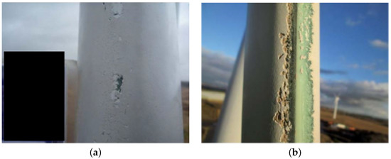
Figure 1.
Minor (a) and major (b) erosion damage on the leading edge of wind turbine blades (reprinted from [12]).
Typically, the leading edge of a wind turbine blade is protected using some form of polymeric coating or tape, referred to as a leading edge protection system (LEP). LEPs are susceptible to environmental conditions during erosion. Temperature sensitivities are particularly common in polyurethane (PU) coatings, with their low glass transition temperatures. In recent solid particle erosion tests, PU coatings have exhibited varying erosion behaviours at a range of temperatures (−30–100 °C) [5,13]. This performance is largely dependent on coating composition and, although some of the temperatures used were outside of typical operational values during rain events, these results exemplify their temperature sensitivities. Thermal cycling and ageing can also affect mechanical properties, further highlighting the need to understand the impact conditions [9,14,15,16,17,18,19].
During rain events, the relative humidity is often high. This atmospheric moisture can interact with polymers to a varying degree. Degradation from humidity fluctuations through water ingress and hydrolysis can temporarily or permanently change mechanical properties [14,15,18,19,20,21,22]. Hydrothermal ageing is well documented too within pure composites [23,24]. However, to the authors’ knowledge, there have been no investigating the influence of humidity or hydrothermal ageing. Furthermore, as wind turbine blade surfaces contain two or more different polymers (at least one LEP layer and the composite), even if the top layer is not affected by humidity, another LEP layer or the composite beneath may potentially absorb water, leading to swelling, which could delaminate or fatigue the interface between layers.
Impurities in rain can also lead to chemical reactions and, with the prevalence of acid rain in northern Europe and sea salt aerosols in coastal and offshore sites, this contribution to the erosion process requires further investigation. In northern Europe, sulphuric and nitric acids are the most common, typically from burning fossil fuels or agricultural sources, respectively. Sea salt aerosols are predominantly composed of chloride (Cl), sodium (Na), sulphate (SO), magnesium (Mg), calcium (Ca), and potassium (K). Salt concentrations are typically much higher than acidic pollutants and are of interest in situations where materials (including polymers) are prone to corrosion [15,16,24]. Recent evidence [12,25,26,27] suggests enhanced degradation due to the presence of sea salt, acidity or at sites in close proximity to quarries. The influence of salt will be more pronounced at sites near the coast or offshore. Exposure to other pollutant concentrations, such as particulate matter and air pollution, is irregular, site specific and changes over time in relation to the pollution from factories, vehicles and other sources. Without the appropriate data, addressing these other pollutant influences becomes difficult.
The recent DNVGL-RP-0171 recommended practice [28] for Rain Erosion Testing (RET) sought to standardise the reporting of these environmental conditions and other aspects. It recommends documenting chamber pressure and temperature, sample temperature and water temperature and quality, as well as the accelerated ageing parameters extreme temperatures, UV exposure, humidity and salt spray. However, exposure to these conditions occurs simultaneously and during rain erosion, creating synergistic effects that are yet to be properly documented. The resultant effects could be severe and further enhance degradation mechanisms [12,15,16,18,25,29,30,31,32,33].
This paper will focus on Ireland, where rain is predominantly orographic or stratiform. As noted by other authors [10,31,34], orography strongly influences rainfall in Ireland (compare Figure 2a,b). Wind from the west, south-west and south typically brings in wet Atlantic weather, with annual rainfall on the west and east coasts in the range of 1000 mm–1400 mm and ∼700 mm, respectively. Rainfall is highly seasonal with winter monthly precipitation on the west coast reducing from 150 mm to 50 mm in the summer. Conversely, monthly precipitation on the east coast remains ∼60 mm throughout the year [10,31]. Rain is typically characterised using rain intensity and exposure time, with size distributions (e.g., the Best distribution [35]) for droplet diameters at a given intensity. Rain intensity can be determined using empirical methods, such as rain gauges, at discrete locations. However, this is not feasible for determining rain intensity accurately over the island of Ireland with reasonable temporal resolution. Weather radars are much more appropriate. However, they suffer from artefacts produced by physical objects, such as buildings or wind turbines. One feature can also be obscured by another between it and the radar station and their accuracy degrades with distance from the station itself, requiring the creation of mosaics from multiple radar stations. Signal processing can reduce spurious data outputs and significantly clean the data and calibration using data from the few rain gauges available is effective and helps to remove artefacts [36,37]. The use of radar composites is therefore beneficial and at this present time the simplest, widely available method to generate rain intensity maps for large areas. Site specific rain intensity histograms can be generated from these data, and when coupled with wind data can provide an effective tool for rain erosion lifetime estimation (either by estimating the impact kinetic energy or by modelling material fatigue from impact numbers) [38] or instead can be used to implement methods such as the Erosion Safe Mode (ESM) [39]. However, further calibration work for the radar network in Ireland is required and, currently, the data available are insufficient.
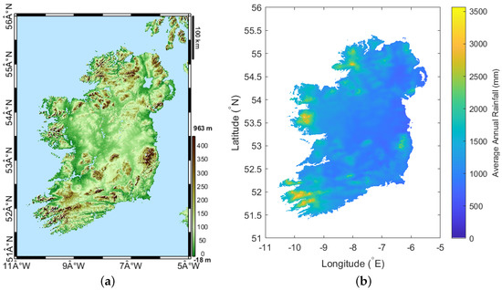
Figure 2.
Topographical data (a) obtained from NASA and average annual rainfall data for the 30 year period 1981–2010 (b) obtained from Met Éireann [40] were mapped using the READHGT function [41] and MATLAB’s [42] imagesc function, respectively.
This paper seeks to address knowledge gaps in the rain erosion process, particularly the approximate magnitude of impact numbers and annual impact kinetic energy, droplet size, temperature, humidity, ion concentrations (sodium and sulphate) and pH, as well as how these parameters vary geographically across the Island of Ireland and annually. Areas which are more prone to damage from rain erosion will be highlighted and site specific conditions can be characterised. Furthermore, seasonal variations in weather patterns may help to identify periods of enhanced or reduced erosion, as well as other degradation mechanisms. Results from this work will also seek to inform RET protocols. This will pave the way for future work to fully understand the influence of these conditions on the rain erosion phenomenon.
2. Methodology
2.1. Rain Erosion Modelling
Currently, rain erosion lifetime prediction uses two main models—either kinetic energy, , or the Springer/water-hammer/fatigue model. The kinetic energy model benefits from considering droplet diameter, without directly considering the aerodynamic influences on droplet shape, impact physics or material characteristics. However, it has had limited application, possibly due to the lack of knowledge on how energy is transferred, absorbed and dissipated. The Springer model [43] has had reasonable acceptance, with authors such as Eisenberg [44] reporting a good fit with reality. However, the model was developed for brittle and elastic materials, fails to consider droplet diameter and, in order to understand a material’s performance, it must first be characterised, which is cumbersome.
The Springer model states that impact pressure is given by the modified water hammer equation:
where the variables ρ, C and V are the density, speed of sound and velocity, with the subscripts L and S referring to liquid and solid, respectively. The impact pressure is linked to the acoustic impedance, Z:
which is in turn linked to a material’s stiffness. If the environmental conditions are known and one accepts the Springer model [43], as in Pugh et al.’s work [19], the lifetime of a specified turbine at a location can be estimated. However, in order to validate the model, rain erosion must be assumed to be a fatigue problem, with the endurance limit determined through a whirling arm RET program over a range of velocities. This maps the number of cycles to failure, N for a given impact pressure, S, generating an S-N curve. n will be used in this paper instead of N, accompanied by the following subscripts: A, meaning annually at a specified speed range; AR, meaning annually at rated speed; and R, meaning at rated speed over a specified time period.
According to Springer’s model, stiff materials, such as gelcoat materials (epoxy or polyester, tensile strength = ∼97 MPa [45] and ∼123 MPa [46], respectively), are more prone to damage, particularly if cracks or defects are present, with impact pressures often close or even higher than their tensile strengths (Figure 3). Softer, viscoelastic materials (e.g., PU) are preferred for their significantly reduced impact pressures. However, the model was not developed for this type of material, presenting further problems. In order to develop and validate models, further work must be carried out to compare inspection reports and failure rates with results computed using impact conditions and environmental data. The variation of impact pressure with impact velocity for a range of materials can be seen in Figure 3.

Figure 3.
Using Equation (1) and data obtained from Slot et al. [47], the impact velocity for droplets is plotted against the impact pressure for LEP coating materials (UP, unsaturated polyester; EP, epoxy and PU, polyurethane). Different plots of each polymer represent slight variations in composition, which lead to different acoustic impedances (given by Equation (2)).
In order to understand the influence and variation of droplet diameter, a size distribution must be used. The most common, termed the ‘Best distribution’, is generally accepted [35]; however, recent investigations [48,49] question its accuracy and applicability. As discussed by Herring et al. [48], Best’s work is the collation of data from two different manual methods. Both are subject to human error and had small data collection time periods, as consecutive droplets can interfere with one another, producing inaccuracies. These techniques also have a limited size resolution of 0.5 mm, reducing their applicability to low rain rates (<1 mmhr), where most droplets are between 0 mm and 2 mm. In spite of these disadvantages, the Best distribution is widely accepted and is relatively simple to implement, making it a good basis to build upon. Rain Erosion Testing (RET) programs commonly use worst-case scenario conditions of ∼25 mmhr, with a droplet size of ∼2 mm, as this is the respective mean size [28,43]. However, further work characterising the influence of droplet diameter on the erosion process is required as well as understanding the range of realistic droplet densities, , that appear in nature. A more detailed discussion of this is beyond the scope of this paper though. The recent development of a rain texture model now enables the prediction of number of impacts, n, and therefore lifetime of the leading edge [50].
Traditionally, interpolation methods such as kriging, have been used to create geospatial rainfall maps for large areas (Figure 2b). Weather processes are complex and these methods rely on relationships that are not fully understood. So, producing accurate, detailed maps for rain intensity with a high temporal resolution is not possible. However, reasonable annual and monthly rainfall maps can be produced. Although lacking the histographic rain intensity information, they do indicate areas that are more prone to rain erosion. Instead, until more data are available, mathematical models must be developed to predict erosion.
The probability of an extreme weather event is identified using return period rainfalls, indicating the maximum rainfall experienced at a site within a specified return or time period. Developed by Fitzgerald [51] and currently used by the Irish Meteorological office (Met Éireann), the model covers the island of Ireland. It not only determines the maxima, but acts to scale what is considered an extreme event for a location. Sites with higher values experience higher intensity rain more often, as confirmed by comparing Figure 2 and Figure 4. Fitzgerald [51] confirms this, noting the distinct correlation between average annual rainfall (Figure 2b) and median yearly maximum 24 h rainfall (Figure 4b).
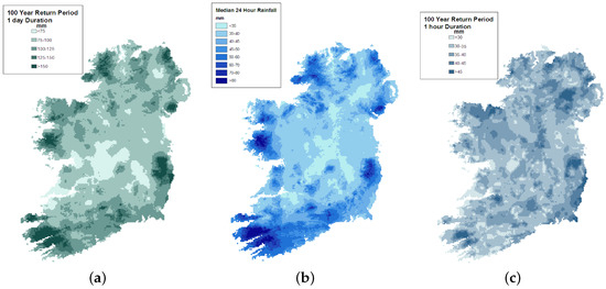
Figure 4.
Rainfall return period mapped for (a) 100 year return, 1 day duration; (b) 1 year return, 1 day duration; (c) 100 year return, 1 h duration. Mapped by Fitzgerald for Met Éireann for the island of Ireland. Reprinted from [51].
As higher intensities produce higher densities, they cause more damage, regardless of whether the damage process is dictated by impact force or kinetic energy. As will be discussed later, if the damage process is controlled by kinetic energy, larger droplets would also cause more damage from a single impact and the compounded effect of both more droplets and larger droplets would accelerate deterioration further.
2.2. Rain Texture Model
The rain texture model proposed by Amirzadeh et al. [50] will be used here. The model uses the relationship first proposed by Best (Figure 5) [35]. As stated by Best, droplet diameters, d, are considered to be accurate above the 10th percentile, , and below the 95th percentile, . So, and were truncated.
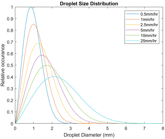
Figure 5.
Droplet size distribution for different rainfall intensities, produced using the Best distribution.
Amirzadeh states the droplet density (droplets m) has a Poisson distribution about the equation:
As Equation (1) is exponential, initial increases in rain intensity lead to proportionally higher densities than at higher intensities. Figure 4c highlights that intensities of >30 mmhr are improbable during the life time of a wind turbine for more than 1 h, and that even intensities >10 mmhr only occur at most for 25 h a year in few locations [37]. Using Equation (3), realistic densities would be in the range of 35 droplets m ( mmhr)–69 droplets m (10 mmhr). As in Amirzadeh et al.’s work, a stochastic spatial droplet distribution is assumed. The result of the model is a 3D distribution of rain droplets.
2.3. Weather Station Data Analysis
Hourly station data obtained from 23 of Met Éireann’s synoptic weather stations located around the island of Ireland will be discussed (Table 1 and Figure 6) [40]. All measurements were recorded at ground level, except for wind speed, which was measured using a 10 m wind mast. For simplicity, each of the weather stations will be assumed as though they were a 100 m diameter wind turbine, with the recorded measurements at hub height and the RPM curve taken from Letson et al. (Figure 7) [38]. Finally, it was assumed the tip of the wind turbine blade is a 10 cm × 10 cm flat plate [52], with all impacts occurring perpendicularly when the blade is horizontal. The influence of wind on the droplet, falling velocity and, due to a lack of data, impact efficiency will all be ignored.

Table 1.
List of stations, country, station type (W—weather, C—rain chemistry), latitude (X), longitude (Y), sample collection height (add 10 m for wind data, Z) and period of time series.
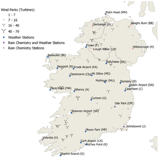
Figure 6.
A map of Ireland with all known wind turbine parks in both the Republic of Ireland (ROI) and Northern Ireland (NI), marked. The 23 weather stations and the 8 rain chemistry stations used in this paper are also marked.
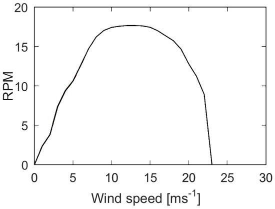
Figure 7.
Wind turbine RPM curve adapted from [38]. The turbine rotates at an approximately rated speed over the wind speed range of 9 ms–16 ms.
It is possible that the wake of upwind turbines influence droplet impact pathways, as well as some level of deflection caused by the boundary layer surrounding the wind turbine blade, which may lead to droplet break up or other effects not considered here [43,53]. Furthermore, the threshold diameter below which droplet deflection due to inertia begins is ∼0.2 mm and the lowest droplet diameter projected is 0.2 mm due to the selected size resolution [44]. The actual influence of blade curvature on impact kinematics is generally considered to be low and it is only significant for larger droplets and in smaller wind turbine blades [54]. This may, however, present a bigger issue for the highly curved samples used in RET. The rain gauges used here were only able to measure precipitation and not, type (hail, snow, etc.) and so for the sake of simplicity, all precipitation will be assumed to be rain. Certain stations did note different weather events; however, detail was limited and so this was not considered.
The data were filtered to remove any data points with missing sensor outputs for either temperature, humidity, wind speed or rain. All data, where the wind speed sensor output was 0 ms, above the cut off speed or where there was no rain, were then removed.
To generate the tip speed, the wind speed was taken and, using the relationship below (Figure 7), an RPM was calculated. The tip speed was then given by:
where is the RPM and D is the wind turbine diameter in meters. A 3D droplet distribution was generated using the rain texture model for each hourly rain data point. Using , the number of revolutions per hour was then generated and combined with the swept volume, v, of the blade tip per revolution:
where A is the frontal area of the wind turbine blade tip. This gives the swept volume per hour. This volume was then combined with the 3D distributions to produce a distribution of droplets impacted over that hour, with their respective impact speeds. The data were then either compiled over the time duration for each station and normalized giving annual results or compiled monthly across all stations and averaged, giving an average month at an average station. Due to the limited resolution of the wind speed measurement apparatus (nearest ms), the bin size for impact velocity was much larger than desired.
As other authors have reported that the wet weather primarily comes from the Atlantic and that the wind direction is predominantly westerly, south westerly and southerly, a series of least squares linear regression models were developed as a basis to investigate the relationship between geographical parameters (longitude, X, latitude, Y, and altitude, Z) and rainfall characteristics (impacts at each speed bin, , total annual kinetic rnergy, , mean temperature, T, and mean humidity, H) with and without MATLAB’s ‘Robust’ option [42]. In each case, coefficients of determination were then calculated. The resulting models were then mapped over the island of Ireland geospatially.
Due to the wealth of data generated, data from three stations will also be presented—A, MA and N. They were selected as they surround the Galway Wind Farm. It is the largest onshore wind farm in Ireland and is on the west coast of Ireland and so, is subjected to higher winds and rain, and therefore erosion. This will be followed by a brief profile of the park using the regression models.
2.4. Rainwater Composition
During the period 2010–2018, there were eight stations sampling precipitation chemistry in Ireland—three sites in Northern Ireland (NI) and five in the Republic of Ireland (ROI) (Figure 6). The NI sites were sampled on a multi-day basis, ranging from 6 days to 29 days. The ROI sites were sampled daily. All sites contribute data to the co-operative programme for monitoring and evaluation of the long-range transmission of air pollutants in Europe (EMEP) [55], except Hillsborough and Beaghs Burn. All three sites in NI contribute to the UK Eutrophying & Acidifying Network (UKEAP) and the five sites in ROI additionally contribute to Ireland’s Atmospheric Composition and Climate Change Network [56]. Data for the respective sites were available from EBAS (provided by EPA (Ireland) [57], Met Éireann [40]) and UK-AIR [58].The NI sites are operated by Ricardo Energy & Environment on behalf of the UK Department for Environment, Food and Rural Affairs. The sites within ROI are all operated by the EPA, except Valentia which is operated by Met Éireann. The pH of rainwater collected from these sites, as well as sodium and sulphate ions (representing sea salts) present within the samples will be analysed. Acidity and ion content were initially investigated month by month. With no apparent variation in acidity month by month, annual results are instead reported. Due to the limited number of stations, understanding a clear geographical pattern proved too difficult and was unreliable.
3. Results
In the following sections, temperature and humidity results for the model that included rain intensity as well as median droplet sizes, temperatures and humidities were not included. Droplet size resolution was too low, and therefore median results were considered unsuitable. For temperature, there was no appreciable difference for the model that included rain intensity as opposed to just rain events. Median temperatures were in good agreement with mean values. There were, however, some differences between mean and median RH values, but not enough to have significant consequences. The differences were more pronounced for monthly humidity standard deviations, with standard deviations being smaller for the model when considering rain intensity, However, these were not considered significant enough to be included here as they mostly affected spring and summer months at nonrated tip speeds.
3.1. Wind
3.1.1. Geographical Variation
All locations received between and rated speed impacts, annually (Figure 8). MH had the highest of any station, with 99 million impacts. Most stations displayed an increasing with tip speed. Across all stations, the lowest speed bin had the lowest .

Figure 8.
at each site for each impact speed bin, as calculated.
Even stations, such as BA and MP, with relatively few hours at rated speed still managed to receive ∼ impacts (Figure 8 and Figure 9). N had the most rain hours of all stations with 2375 h. However, surprisingly MH had the highest (∼670 kJ) with only 1768 h.
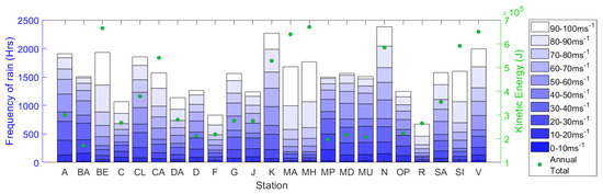
Figure 9.
Number of rain hours and for each impact speed bin, at each station.
The highest (0.48) for both and regression models was for two predictor variables, X and Y. There was little correlation (<=0.30) between and other geographical parameters. In this case, the RMSE was particularly high (∼132 kJ), equal to ∼20% of . Interestingly, the largest (0.57) was for and all three predictor variables.
Using the regression estimates, is given by:
Using the model, Galway wind park would have an of ∼585 kJ. By extrapolating the models, the three wind parks with the highest would be Clydaghroe (∼673 kJ), Kilgarven (∼662 kJ) and Coomacheo (∼658 kJ).
Maximum droplet diameters for most stations across all velocities were in the range of 3 mm–4 mm, (Figure 10a–c, with the exception of a few stations with larger droplet sizes in the lower velocity ranges such as N. Generally, intensities greater than 6 mmhr were uncommon, occurring for <1 h, across all speed bins and stations (Figure 10d–f). Most events were concentrated around the lowest intensity bin (0 mmhr–0.5 mmhr). Of the three stations selected, N had the highest droplet diameter with 5 mm (Figure 10c).
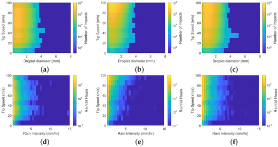
Figure 10.
Annual impact distributions for the sites: A (a), MA (b) and N (c) for each given speed bin. Total annual number of rainfall hours at a given rain intensity, for a given speed bin for A (d), MA (e) and N (f).
Across all stations, the mean and standard deviation of droplet size increased with velocity (Figure 11). In the rated bin, all stations displayed a mean droplet size in the range of 0.95 mm–1 mm, with a large standard deviation in the range of 0.8 mm–0.9 mm.
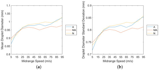
Figure 11.
The variation of mean seen in (a) and standard deviation in (b) for droplet diameter with the midrange tip speed of each bin for stations A, MA and N, as calculated by the model.
3.1.2. Annual Variation
Throughout the year, there was a pronounced cyclical pattern in the high velocity impacts. was highest during January and December, with ∼ impacts, and lowest during July with ∼ impacts (Figure 12).
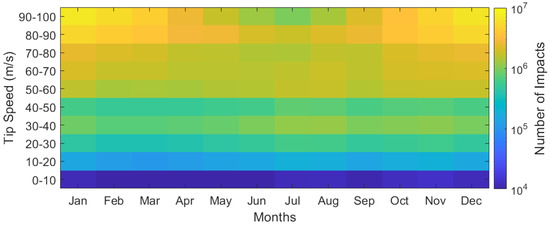
Figure 12.
for each month, for each speed bin, as calculated.
Rated wind speeds during rainfall occurred ∼10 times more often in winter than in summer (Figure 13), with more rain events during winter months (October–March) than summer months (April–September), particularly at higher speeds. This results in considerably more in winter months. December averaged the highest of any month (∼63 kJ), compared to July, which had the lowest (∼22 kJ). Interestingly, the fewest hours occurred during June and not July, with 99 h. On average annually, there were 1552 h of rainfall.

Figure 13.
The number of rain hours and for each impact speed bin for each month.
Droplet size distributions varied significantly between the summer and winter months. There were more events at high speeds during winter and higher intensity events at lower speeds during summer. During winter, rated speed events on average had higher intensities, increasing the average droplet diameter. The increased high intensity events during summer at lower speeds increased the maximum droplet diameter observed. Summer also had fewer rated speed rain events, resulting much fewer impacts (Figure 14).
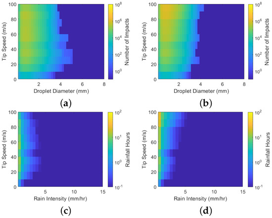
Figure 14.
The average impact distributions during the months July (a) and December (b), respectively, for each given speed bin. (c,d) show the total number of rain hours for a given speed bin during the same periods.
The highest rain intensity was recorded in July, with an intensity of ∼41 mmhr. The event occurred when the tip speed was between 20 ms and 30 ms. In fact, the highest intensity event at rated speed across all data analysed was ∼21 mmhr, during September, which, when normalised and averaged, occurred for 0.002 h. Most high intensity events occurred during summer months, when turbine speed was suboptimum. This is illustrated by the elongation of the size distribution at speeds below 60 ms on Figure 14a. Diameters mm were infrequent at rated speed (<1000 per year) (Figure 14a,b). As in Section 3.1.1, rain intensities much higher than 6 mmhr rarely occurred, with most rain events concentrated around the lowest rainfall intensity bin.
As in Section 3.1.1, in all months the mean and standard deviation of droplet size showed an increase with velocity (Figure 15). For all months at rated speed, mean droplet size was between 0.95 mm and 1.05 mm, with a smaller standard deviation range of 0.8 mm–0.88 mm. Interestingly, mean and standard deviation curves were steeper for winter months, whereas summer month curves were flatter.
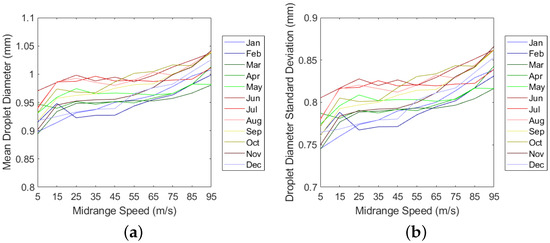
Figure 15.
The variation of mean (a) and standard deviation (b) for droplet diameter with the midrange tip speed of each bin for each month, as calculated by the model.
3.2. Temperature
3.2.1. Geographical Variation
At low rain intensities, temperatures during rain events were well distributed. Common temperatures (≥1 h) at the lowest rain intensity bin ranging between 5 °C and 15 °C (Figure 16). Mean temperatures started at just below 10 °C and, in contrast to standard deviation, as rain intensity increases, it skewed upwards (Figure 17). Precipitation events with temperatures below zero or exceeding 20 °C occurred very rarely (Figure 16).

Figure 16.
Average annual temperature/rainfall (a–c), temperature/rainfall/tip speed (d–f) and temperature//tip speed (g–i) distributions for stations A, MA and N, respectively.
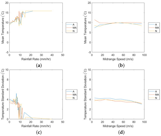
Figure 17.
Mean (a,b) and standard deviations (c,d) of data presented in Figure 16 against the midrange tip speed of each bin, for the respective stations.
Temperatures between 5 °C and 15 °C were relatively common across all velocities (Figure 16). There was little temperature variation with tip speed; however, standard deviation had a decreasing trend (Figure 17). K had the lowest mean temperature across many of the speed bins, whereas SI and V mostly had the highest. Even temperatures as low as ∼1–3 °C had relatively frequent impacts ∼105–106 at some stations. In total, 77% of stations had mean and median temperatures within 8–10 °C across all speeds. This tightened when reducing the scope to just rate speed values (Table 2).
Table 2.
Distributions of mean and median temperatures for rainfall hours and across all stations.
Using the mean temperature at a given speed and its respective , the model with the highest value was found to be for the predictor variables, Y and Z, and the response variable, T, at rated speed, at 0.73. T is given by:
Using the model (Equation (7)) to estimate T for Galway wind park would give ∼7.6 °C, with the same wind parks described in Section 3.1.1 with T = 6.7 °C, 7.2 °C and 6.9 °C, respectively.
3.2.2. Annual Variation
In contrast to Section 3.2.1, at low rain intensities, the temperature distribution is much narrower (Figure 18). In July, common temperatures at the lowest rain intensity bin range between 13 °C and 16 °C. However, in December, this range is between 5 °C and 10 °C. Mean temperatures during each month are much flatter with rain intensity (Figure 19). During July and December, the distribution profiles still skew during higher intensity events downward and upward, respectively (Figure 18). However, temperatures during summer events displayed an increasing mean with intensity (Figure 19). The standard deviation does reduce too, with increasing rain intensity (Figure 19).

Figure 18.
Average annual temperature/rainfall (a,d), temperature/rainfall/tip speed (b,e) and temperature//tip speed (c,f) distributions for July and December, respectively.

Figure 19.
Mean (a,b) and standard deviations (c,d) of data presented in Figure 18 against the midrange tip speed of each bin for the respective months.
During summer months, rain events were reasonably distributed across all of the speed bins, with temperatures between 10 °C and 15 °C (Figure 18). However, during winter, most rain events occurred close to or at rated speed (>80 ms), with cooler temperatures ranging between 5 °C and 11 °C. Subzero temperatures were infrequent (<1 h) for all speed bins. In summer months, rated speed impacts (>10) were common at the narrow temperature range of 12–15 °C and rarely exceeded 20 °C (<1 h). However, during winter, rated speed impacts (>10) occurred over a much broader range of 2–12 °C.
As one would expect, average temperatures during summer rain events were higher than winter. Interestingly, mean temperatures increased with turbine speed during winter months. Standard deviations across all speed bins were lower in summer months than winter.
3.3. Humidity
3.3.1. Geographical Variation
During rain events, the relative humidity was predominantly >90% at all stations (Figure 20). This is highlighted for rain intensities of >5 mmhr. RH was particularly skewed towards a value of around 95–96%. Generally, mean RH increased with rain intensity; however, the standard deviation (Figure 21) and minimum/maximum range (Figure 20) decreased. As discussed earlier, some of these decreases in standard deviation will be due to the reduced number of events.
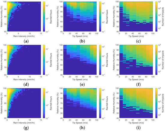
Figure 20.
Average annual humidity/rainfall (a–c), humidity/rainfall/tip speed (d–f) and humidity//tip speed (g–i) distributions for the stations A, MA and N, respectively.
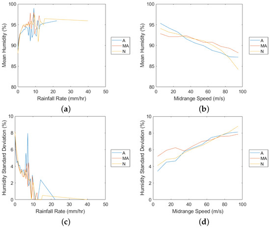
Figure 21.
Means (a,b) and standard deviations (c,d) of data presented in Figure 20 against the midrange tip speed of each bin, for the respective stations.
At most stations, the RH minimum/maximum range increased with tip speed (Figure 20), largely because of a decreasing minimum RH value. Most stations reported RH values as low as ∼75% for at least 1 h. Across all speeds, stations mostly reported mean values above 90% (Figure 21). However, in contrast to rain intensity, with increasing tip speed mean RH decreased whereas standard deviation increased (Figure 21). This meant most rated speed mean values were less than 90% (Table 3).
Table 3.
Mean and median RH distributions for rainfall hours and across all 23 stations.
Using mean RH values for rain events and for , the model with the highest R value was found to be for the predictor variables, Y and Z, and the response variable, H, at rated speed, at 0.52. H was given by:
Using the above model, Galway wind park would have an H = ∼94%, with the wind parks mentioned in Section 3.1.1 having a mean RH of 103, 101 and 102%, respectively.
3.3.2. Annual Variation
Rain intensity varied with RH in the same manner as in Section 3.3.1. There was no discernible seasonal pattern and most characteristic trends were the same. The main difference was the increased number of events during winter compared to summer months (Figure 22).
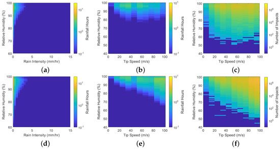
Figure 22.
Average annual humidity/rainfall (a,d), humidity/rainfall/tip speed (b,e) and humidity//tip speed (c,f) distributions for July and December, respectively.
There was, however, a seasonal variation in RH with tip speed (Figure 22). During summer months, there were fewer events at higher tip speeds. RH values were typically higher in upper speed bins and the range covered was significantly reduced. Mean RH values had a more gentle gradient compared to winter months (Figure 23). Interestingly, spring months had lower mean and median values at nearly all speeds, with higher standard deviations in April and May in most speed bins. During winter months, as in Section 3.3.2, the RH range increased with tip speed, with this mainly being due to a decreasing minimum RH value (Figure 22). The mean RH gradient is the steepest for winter months, interestingly having the highest mean RH in the lowest speed bin and almost the lowest mean RH in the highest speed bin (Figure 23). The standard deviation during summer months has a gentler slope in contrast to the rest of the months. In contrast to Section 3.1 and Section 3.2, the influence of including rain intensity is more pronounced. This increased the mean RH in almost all cases (118/120). The highest increase was in April in the highest speed bin with an RH of 0.7%. All cases except one (119/120) had higher standard deviations when excluding rain intensity. The highest increases were in April (30 ms–40 ms) and July (40 ms–50 ms) at 1.6% in both cases.
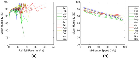
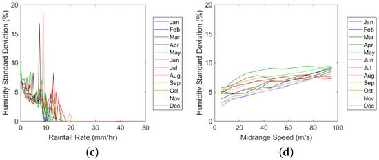
Figure 23.
Mean (a,b) and standard deviations (c,d) of data presented in Figure 22 against the midrange tip speed of each bin for the respective stations.
3.4. Composition
3.4.1. Acidity
Overall, stations mostly displayed an increase in annual mean pH when comparing 2018 with 2010 (Table 4). However the increase was slight in four out of five ROI stations (1.5–8.1%) and there was a decrease in one out of five (−3.2%). All NI stations displayed an increasing trend, with typically larger increases (6.9–18.1%). The range of values in annual mean pH in NI was also higher (5.5–6.5) than ROI (5–6), indicating that NI is less acidic than ROI.
Table 4.
Mean pH values at year station across the selected years 2010–2018. Empty cells in the table are due to unavailable data.
All stations had a reasonably low standard deviation of approximately 0.5 across all years. The median values also tracked the mean values very closely, with the minimum value across all stations for all years reported as ∼3.73 (J, 2014). No seasonal variation or correlation with precipitation volume was found.
3.4.2. Salinity
The ratio of mean sodium to sulphate concentrations was ∼10 (Figure 24), indicating that sea salts dominate rainwater chemistry. The mean sulphate concentration trends generally follow that of sodium concentration, with peaks at the start of the year, decreasing through summer, then rising back up towards the end. The standard deviations are very high (larger than some of the mean values) at ROI stations for some months in both sodium and sulphate. The sites closest to the west coast (MH and V) have particularly high sea salt concentrations. All stations in the ROI had larger maximum concentrations for both ions than stations from NI (Figure 25).
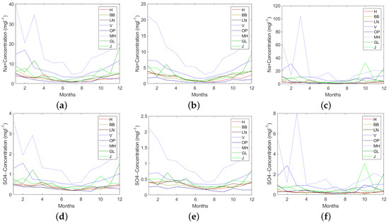
Figure 24.
Annual variations in the mean (a,d), median (b,e) and standard deviation (c,f) of sodium and sulphate ion concentrations, respectively, in rainwater collected at each site.
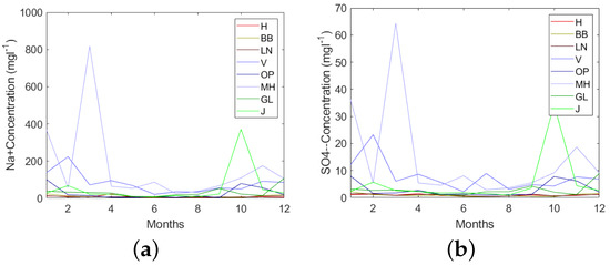
Figure 25.
Maximum values reported by the stations of sodium (a) and sulphate (b) ion concentrations in rainwater collected at each site.
4. Discussion
4.1. Wind
The data presented here broadly support the consensus that rainfall across the west coast is considerably higher. Most rain events had low intensities, with most stations (13/23) reporting a trend of increasing rainfall hours with tip speed. In all instances, the lowest speed bin (0 ms–10 ms) had the lowest number of rainfall hours. The rated speed bin usually had either close to or the highest across all stations, with the same increasing trend as rainfall hours. These are likely due to two reasons: firstly, the 90 ms–100 ms tip speed bin covers a larger wind speed range than any other and, secondly, during rated speed operation, the RPM is higher, meaning more impacts per minute. Other authors have noted the synergistic nature of rain and wind [59,60]. The exact reason that some stations did not display the trend of increasing rainfall hours with tip speed is unknown as they did not display reduced rainfall nor mean wind speeds [61].
The influence of rated speed rainfall hours on kinetic energy is quite apparent (Figure 9) when comparing stations such as MP, MD, and MU with SA. All four stations had similar rainfall hours, yet SA experienced significantly more hours in the 80 ms–90 ms and 90 ms–100 ms bins, leading to an increase in kinetic energy of 44–59%. Overall, the equation and data (Figure 26) support evidence reported by others that westerly winds carry much of the wet weather and that orographic enhancement plays a significant role, in increasing rain kinetic energy. However, the inclusion of latitude into the equation reduced , conflicting with the hypothesis that there is a significant southerly component. This indicates that the mountains on the west coast and areas exposed to the wet Atlantic weather are more affected by rain erosion [10,60]. An value of 0.48 shows that the regression model poorly reflects reality. It is likely that relationships between the geographical parameters and kinetic energy are nonlinear, with other factors such as micro-climates influencing localised weather patterns. The limited number of weather stations investigated here will also have some influence. Furthermore, it is problematic in applying this model to mountainous regions where significant variation is expected and data are limited [31,34,37] or in extrapolating it above kinetic energies reported here.
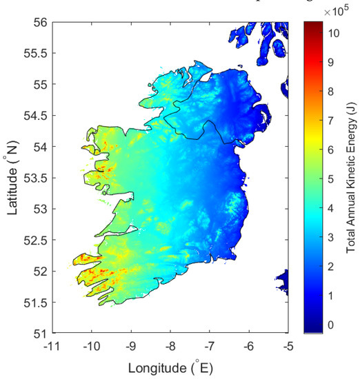
Figure 26.
A total annual kinetic energy map of the island of Ireland, generated using Equation (6), using topographical data obtained from NASA and processed with the READHGT function [41].
When comparing the total annual kinetic energy of sites in Ireland and that produced by Letson et al. [38], the results here display significantly more energy in rain, compared to the sites investigated in the USA, Jm– Jm vs. Jm– Jm, respectively. One reason for this will be the temporal resolution of the data. One should consider two separate cases, a 10 min interval (10 mmhr) and two 5 min consecutive intervals (20 mmhr and 0 mmhr). Calculated droplet concentrations, using Equation (3), differ significantly and average out to be ∼69 droplets m and ∼38 droplets m, respectively. Just in this one instance, the same volume of water would have accumulated, but the second case had an average droplet concentration and therefore n equal to 55% of the first case. If a turbine with the same specifications as outlined here, but with = 15, the from the first and second cases would be 769 Jm and 699 Jm, respectively. Therefore, the reduced temporal resolution of the data here will likely lead to an overestimation of the total kinetic energy at each site as well as the n.
The wind speed data are also limited to hourly resolution and so are the average wind speeds throughout that hour and as is capped to rated speed, the total kinetic energy inside the rated speed bin will be overestimated. This is justified as there will be periods during that hour where is suboptimal, meaning that the impact speeds will be lower, also reducing . There was no attempt made here to convert to the wind speed at hub height. Hub height wind speed is highly dependent on site specific characteristics (i.e., local topology, obstructions, wind direction, etc.), and so mapping erosion potential with this conversion would have added considerable complexity [62].
Upon reviewing wind speed data from Letson et al. [38], the selected wind turbine rarely reaches rated speed, although there were sites here with suboptimal wind conditions, such as BA, where rated speed occurred for just 1.6% during rainfall. The total annual impact energy per m is still approximately 20,000 KJm. Assuming for 1 h , A = 0.01 m, D = 100 m and the rain intensity is such that λ = 50 (∼1 mmhr), with all droplets having a uniform diameter of 1 mm. This would give a kinetic energy concentration of 22,800 Jm, far higher than reported by Letson et al. (0.3 Jm–50 Jm).
The wind turbine RPM curve and blade diameter used should also be considered. Most RPM curves are quite similar in shape but have different rated speed ranges/profiles. The RPM curve taken from Letson et al. may also be for a smaller turbine and, as kinetic energy per impact is proportional to D, this would substantially reduce the tip speed, and therefore impact speed, as well as the kinetic energy compared to that reported here [63]. Their model of impact speed (noted as closing velocity), which includes droplet velocity and blade position, could account for some of the difference too, although it would likely lead to an increase in kinetic energy. However, in spite of the limitations of the model produced here, the ability to compare and contrast each site using the rain kinetic energy provides a useful tool in analyzing the relative erosivity.
The data presented here demonstrate no discernible geographical variation in mean or standard deviation of rain droplet diameter. A clear pattern, however, emerged between mean droplet diameter and tip speed. As the lowest mean diameter occurs during the lowest turbine speed (<10 ms), it implies that very low intensity rain is often accompanied by mild wind and that its presence decreases with wind speed. Two potential reasons for the increase in standard deviation of droplet diameter (Figure 11b) could be a broader range of common intensities at higher tip speeds and that the tails of the distributions become shorter. Mean droplet sizes (∼1 mm, across all velocities) reported here are 50% lower than those typically used in RET or droplet impact simulations (∼2 mm). During RET, samples are subjected to 25 mmhr, high intensity rain, which in nature has a mean droplet diameter of ∼2 mm (as given by the Best distribution). As given by the data, if we accept a mean droplet diameter of ∼1 mm with a standard deviation of ∼0.8 mm, then this would cover ∼68% of the total data. This would imply most RET is conducted under unrealistic conditions, especially when considering rain intensities beyond 10 mmhr very rarely occur at rated speed.
There is strong annual variation in weather characteristics. Winters are characterized by stronger more consistent winds coupled with significantly more rain. Summers tend to be calmer and, on average, dryer. Interestingly, the majority of high intensity events (>10 mmhr) occur during summer months (Figure 27), a phenomenon noted by others [59,64]. As the model specifically looks at tip speed, rather than wind speed, it makes it difficult to understand whether these high intensity events occur during high (greater than max rated wind speed, ∼16 ms) or low winds (less than min rated wind speed, ∼9 ms). On further inspection of the raw data, it can be seen that the majority occurred during low wind (0.75 h), fewer during rated speed wind (0.15 h) and a small fraction occurring during high wind (0.01 h).
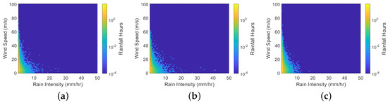
Figure 27.
Frequency distribution of wind vs. rain data for the months of June (a), July (b) and December (c).
The differences in and kinetic energy between summer and winter months can be explained by the following three reasons: the rated speed bin covers a broader range of wind speeds, the wind speeds are more consistently reaching rated wind speeds during rainfall events and there is significantly more rain. This is supported by other authors, reporting strong annual variations in wind speed and capacity factor [65,66], coupled with the change in rainfall [59,64,67]. Upon investigating the frequency of each droplet diameter during December and July, the comparison revealed the influence that winter months have on the droplet size distribution, skewing it upwards. During rated speed events, mean droplet diameters across all months were ∼1 mm. The pattern observed in mean droplet diameter implies that, during summer months, rainfall is somewhat similar across all speeds, whereas, during winter, rainfall intensity becomes heavier on average with increased tip speed. The exact reasoning for this is unclear; however, it is likely in part due to a change in the hydrological cycle. Furthermore, it can be seen that the majority of the larger droplet sizes (>3.5 mm, Figure 14) that exist are unlikely to occur during high speed operation. This is particularly important for modelling droplet impacts, in order to understand the upper limit of what is commonly observed in reality. Overall, the data presented here indicate that the kinetic energy of rain is much higher in winter than in summer and that high intensity events are unlikely to contribute significantly to the rain erosion process.
Erosion mitigation strategies, such as ESM, assume that rain erosion is predominantly caused by a limited number of rated speed, high intensity events [62,68,69]. By comparing the results here and the results of Bech et al. [68], the ∼9 min a year of high intensity rain (>10 mmhr) forecasted would be insufficient for the onset of coating loss at rated speed (79 h at 10 mmhr, stated by Bech). Most rain erosion tests typically last longer than an hour at intensities of 25 mmhr before the incubation period is completed. However, the time resolution of data used here is very limited and erosion is site specific. As stated by Bech et al., the rain intensity of a 1 h period can vary as much as 10 times for convective rainfall, which although infrequent in and around the British isles, provides some context. Work on rain radars carried out by Fairman et al. [36,37] for the British Isles would also suggest that high intensity rainfall rates are more common than observed here (as much as 25 h per year in some locations). So, it is reasonable to assume that higher intensities occur, but are effectively averaged out. Further work must be carried out to investigate site specific rainfall rates using higher time resolution methods such as radar, the results of which should be compared to field data.
Not considered here is the influence of the wind itself on the terminal velocity of the droplet and the direction/impact angle of the droplet onto the blade. Wind acting on a droplet would increase droplet velocity, possibly with horizontal components as high as vertical and impact angles relative to the ground of up to 45° [43,70]. This effect is likely to be of some importance, considering a droplet velocity of up to ∼10 ms, which could increase rated speed impacts by up to ∼10% and the kinetic energy by up to ∼23%.
The model and results here are primarily focused around Ireland; however, the concept of generating mathematical models to characterise erosion could be applied to other countries/geographical regions. It is likely that regions with less exposure to marine environments or large water bodies would produce simpler, more accurate linear regression models. Consequently, with reduced exposure to water, there would likely be less rain erosion.
4.2. Temperature
Mean and median temperatures during rainfall events across most stations displayed a general trend to increase with rainfall intensity. As explained above, higher intensity events typically occur during summer when temperatures are consistently higher. This caused a skew in the overall distribution of the data and the increasing mean/median temperature with rainfall intensity. High intensity weather events usually occur due to an increased air temperature, increasing the amount of water vapour it can contain. This means high intensity events occur due to more specific conditions, which do not usually occur during winter. The standard deviation reduces as these high intensity events require a more selective set of conditions that are atypical for the Irish climate. However, this is beyond the scope of this paper.
The mean and median impact/rainfall temperatures remained relatively constant across all speeds at all stations, although with a slight decreasing gradient as tip speed increased. This is to be expected, as most summer events occurred at lower tip speeds and the converse is true during winter, as discussed above. As expected, there was a reduced temperature at rated tip speed and a higher temperature at lower tip speeds, which can be seen when viewing the differences in minimum and maximum values in the mean. Excluding tip speeds of 0 ms–10 ms−1, the minimum/maximum differences range from 0.4–1.9 °C and 0.4–2.0 °C, for n and Hrs, respectively.
Stations at higher latitudes and altitudes experienced colder events, leading to a lower mean, as displayed by Equation (7) and Figure 28. However, mean rainfall temperatures ranged between 7.9 °C and 11.9 °C for rainfall events between 0 mmhr −1C and 5 mmhr −1C, which is mostly due to Ireland’s location, size and orography (<1040 m). As sites closer to the west coast, with higher altitudes and which are more southerly, experienced more rainfall events, their distributions were more populated. Temperature variations were moderated by proximity to the marine environment, with few regions far from the sea [71], and the linear equation here fails to capture this.
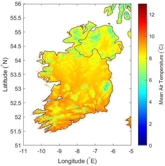
Figure 28.
A mean air temperature map of the island of Ireland, generated using Equation (7), using topographical data obtained from NASA and processed with the READHGT function [41].
The seasonal variation in temperature during rainfall events was to be expected. However, during winter, the trend of a slight increase with rainfall intensity is likely due to the capacity of the air, when warmer, to hold more moisture. This, in turn, leads to heavier rainfall events occurring during warmer temperature periods [72,73].
During autumn and winter, the trend of increasing temperature with tip speed is due to warmer (relatively) sea temperatures, which cause westerly, south westerly and southerly winds travelling over the Atlantic to heat up [60]. Higher temperature gradients, occurring during winter, lead to stronger winds. This can be seen in Figure 27, with wind speed data skewed upwards, meaning that rated speed observations are more common, explaining the increase in temperature with wind speed. Typically, in summer, wind speeds are lower because of reduced temperature gradients [71]. This would also explain the increase in standard deviation for winter months, as wind speeds higher than rated speed are more frequent, especially in the decreasing gradient portion of the RPM curve. This in turn means air temperatures are more likely to have more distributed data points in winter than in summer.
Temperature strongly influences the mechanical properties of temperature sensitive polymers [17,19]. Impacts generating localized heating and fluctuations in air temperature during rainfall may well lead to accelerating the aging process. As discussed by Pugh et al. [19], Polymeric materials typically used as coatings may have glass transition temperatures in the range of 0–30 °C. In practice, this means the behaviour of coatings will change over the operational range of a wind turbine.
Temperature stated here is the air temperature and as previously discussed, all precipitation is assumed to be rain. There are a limited number of events in the data, where the temperature falls below 0 °C and, as noted by others, snowfall is a small proportion of overall precipitation in Ireland [59]. This assumption, therefore, did not skew the results.
4.3. Humidity
Higher intensity rainfall events tend to occur when atmospheric humidity is increased, as is shown by the data. This is in part because higher intensity events require increased levels of water vapour in the air, but also partly because when rain falls, evaporation begins, increasing ground level humidity. The data presented show a strong latitude and altitude influence (Figure 29) and, as above, humidity is strongly influenced by proximity to the coast. These factors mean that the linear regression model (Equation (8)) failed to capture the nonlinear geospatial variance of humidity, which explains the low coefficient of determination (0.52). This failure is highlighted with mountainous regions finding poor representation, leading to humidities of above 100%.

Figure 29.
A mean relative humidity map of the island of Ireland, generated using Equation (8), using topographical data obtained from NASA and processed with the READHGT function [41].
It was expected that RH data reported at stations would decrease with tip speed, partially due to rainfall seasonality, with summers having higher rain intensities at lower wind or tip speeds. These high intensity events would also explain the increased standard deviation in summer months at lower speeds compared to winter. The trends observed in Figure 23 of a decreasing mean humidity with tip speed conflict with the results of Figure 15 as they indicate that mean rain intensity decreases with tip speed. According to the Penman evaporation potential theory, evaporation rates are dependent on humidity, wind speed and air temperature [74]. Summers are characterised by increased temperatures, reduced RH and lower wind speeds, whereas winters are characterised by reduced temperatures, higher RH and higher wind speeds, with more rain events at the rated speed [75]. It is possible that this complex process of evaporation may account for the variations experienced here; however, investigating this is beyond the scope of this paper.
During impacts from projectiles, heat is generated in the target material. Humidity can enhance the heat transfer from materials into the surrounding air, influencing the erosion process, particularly with high impact rates [76]. Humidity is a problem for polymers, causing degradation through hydrolysis and water ingress. This process can be catalysed by salts, reducing the mechanical properties of wind turbine blade materials and enhancing erosion damage [15,16,27].
4.4. Composition
Due to the limited number of stations available, no reliable geographical correlation was attainable for either pH or ion concentration. Ahern and Farrell [31] reported an increase in anthropogenic pollutants towards mainland Europe with mean pH values in the range 4.62–5.25, with a weighted mean of 4.98, for the 1994–1998 period. The values reported here are far higher and over the last 22 years, emission compositions across Europe have significantly changed, making their results incomparable. All stations here reported only slightly acidic pH levels, meaning any influence is likely to be limited. There was no apparent seasonal variation in pH levels nor was there a discernible year on year trend in ion concentration.
As most sodium within rainwater is of marine origin, and the ratio of sodium to sulphate ions is quite large, this indicates precipitation chemistry is dominated by marine ions. The stations are also all relatively close to the sea. This limits the applicability of the results to inland regions. However, it highlights the significance for onshore parks in coastal countries such as Ireland, the UK, Denmark, etc., as well as offshore parks. The saline content, across all stations, is much higher during the winter than summer when precipitation levels are much higher. Sea salt aerosol generation is controlled by the wind, which generates waves, splashing onto rocks and breaking. This forms bubbles and foam, which in turn generates aerosols. A more detailed explanation is available from Tryso et al. [32].
Malin Head and Valentia typically have higher sea salt concentrations, likely explained by their proximity to the west coast. During the winter months, the westerly Atlantic winds begin to pick up, driving sea salt production. All ROI stations had larger maximum values than NI stations, largely due to data collection methods. In NI, data are collected over multi-day periods compared to ROI, where data are collected on a daily basis. Therefore, the NI data average out any large peaks that would otherwise occur, which explains why the mean and median values are of the same magnitude.
As noted by Rasool et al. [27], data from RET experiments show enhanced degradation in both the presence of saline and acidic solutions. Pugh et al. [25,26] supports this, noting that the presence of salt within the working fluid appears to enhance rain erosion through the crystallisation of salts on the surface. The data presented by Law and Koutsos [12] support this with wind parks closer to the coast displaying more severe damage in a shorter period than those in remote regions. Law and Koutsos also investigated sites with nearby quarries, which displayed enhanced erosion. This could be due to the high particulate matter air pollution present in areas with operating quarries. Networks such as the EMEP are unsuitable for determining these relationships with their reduced station numbers, remotely located from strong pollution or particulate sources.
Research indicates that lower humidities lead to increased levels of pollen, PM2.5 and PM10 particulates in the air and that deposition is far higher during rainfall events. Therefore, the results here imply more chemical and particulate depositions occur during lower wind speed rainfall events [77,78,79].
With this observation network and the concerted effort over the past 50 years to reduce acid rain prevalence within Europe, rain pH is likely to remain constant or increase. Salt content, however, probably will not change and the influence and prevalence of particulates and other pollutants require further investigation.
Currently, there is a lack of understanding of synergistic effects between chemical components, temperature, humidity and other testing parameters. To the authors’ knowledge, there have been no RET studies which have sought to monitor the combined influence of water composition, temperature and humidity on rain erosion, with only a few studies investigating acid rain or artificial seawater. This highlights the lack of understanding of these synergistic effects. With the expansion into offshore in and around the UK as well as elsewhere, further work is required.
4.5. Galway Wind Park
Using the model data presented here, Galway wind park is placed in a moderate-highly erosive environment, with a total annual rain kinetic energy of ∼585 kJ and, during rated speed impacts (>90 ms), a mean humidity and temperature of ∼94% and ∼7.6 °C, respectively. Based on the results, this would also likely receive 10–10 impacts, but it was not possible to develop a model and give a prediction. Without field data, model validation is not possible. Further work on temperature and humidity effects is required to understand their relationship to erosion.
5. Conclusions
Presented here is the first attempt to geospatially map erosion environments and erosivity over the island of Ireland. The models developed here suggest that the western region of Ireland is a particularly erosive environment, especially in the mountainous regions west of Cork, i.e., Kerry and Galway, where kinetic energy was predicted to be the highest. Common impact numbers estimated using the rain texture model and RPM curve ranged between 10 and 10. The warmer southern regions are much less susceptible to cold weather events (0–5 °C) compared to the northern and elevated regions, which will likely lead to differences in the erosion performance of some materials. The more humid, mountainous regions imply that chemical deposition may be less likely during rainfall events, but also indicate that material performance may be reduced. Coastal regions are much more susceptible to chemical attacks, with blade materials and coatings potentially undergoing enhanced hydrolysis. Acid rain is likely to be of limited influence due to the neutrality of pH values observed over ireland. Overall, the results here indicate that mountainous regions are the most likely to experience severe erosion, especially in the west/south-west of Ireland. However, further work is required in order to confirm this.
Importantly, the results of this paper suggest that RET protocols, such as [28,80], should be revisited. The influence of using unrealistic rain intensities and droplet diameters is unknown and, with the time dependent nature of viscoelastic materials, this could be key to further understanding rain erosion. The test chamber humidity should be recorded and further work investigating the influences of rain intensity, temperature, humidity, composition as well as droplet diameter should be undertaken. Complex architectures of viscoelastic materials layered in coating systems mean these factors should not be overlooked. Future RET studies should also focus on understanding the influence of synergistic effects of the environment on rain erosion.
Seasonal variations in both rain kinetic energy, temperature, humidity and chemical composition indicate that erosion occurs differently depending on the time of year. Rainfall amounts are significantly reduced in the summer and enhanced in the winter in terms of rain events. Rainfall intensities peak in the summer; however, this is usually with suboptimal wind speeds. The majority of rainfall intensities are low and, according to the analysed data, rated speed, high intensity events, at >10 mmhr, are unlikely to occur, especially in winter. At rated speed, temperatures and humidities are often much lower during winter than summer, which will influence material performance. Sea salt aerosols are much more prevalent during winter months, which, when combined with the decreased humidity at rated speeds, could lead to increased depositions and therefore enhance damage processes. The results here indicate that the erosion process is much more severe during winter.
The limitations of the study can be summarised as follows:
- Limited data time resolution likely led to over estimates in both rain kinetic energy and impact numbers, which in some cases could be 10 and 82% higher, respectively.
- The reduced number of stations reduced the accuracy of the models and monthly estimates. There was also a lack of weather station data from higher altitudes, which created bigger uncertainties for extrapolating the models.
- Data were measured at ground height or at 10m for wind speed. In future, it would be desirable to either use a conversion to estimate hub height parameters or to measure data at closer altitudes to hub height.
- The wind turbine RPM curve used was not necessarily applicable. As RPM curves are highly dependent on wind characteristics, this may cause more or less degradation than predicted here, producing uncertainty in the model.
- The limited number of chemical analysis stations meant that understanding geographical and annual variations proved difficult. More stations or the use of a chemical deposition model would have improved the understanding of rain composition and how this varies.
- Linear regression was likely unsuitable for modelling these impact condition parameters. In future, either nonlinear regression models or the use of RADAR or numerical weather prediction models to estimate erosion would provide a better understanding of impact conditions geospatially and annually.
Future work should seek to improve the rain texture model by finding the most appropriate droplet size distribution and droplet density equation, as well as the inputs to the model, either through using a numerical weather prediction model or radar data, making sure to adjust for hub height differences. The geospatial modelling of rain erosion will be key in understanding which turbines require more protection than others and which sites are more prone. Laboratory work aiming to understand the influence of impact conditions on RET results could explain the variation in lifetime seen in the field. Finally, combining these two areas of research would provide a useful tool in determining and ultimately increasing the lifetimes of wind turbine blade materials.
Author Contributions
Conceptualization, M.M.S. and J.W.K.N.; methodology, J.W.K.N.; software, J.W.K.N.; validation, J.W.K.N.; formal analysis, J.W.K.N.; investigation, J.W.K.N.; resources, M.M.S.; data curation, J.W.K.N.; writing—original draft preparation, J.W.K.N.; writing—review and editing, M.M.S., J.W.K.N. and I.Z.; visualization, J.W.K.N.; supervision, M.M.S.; project administration, M.M.S. and I.Z.; funding acquisition, M.M.S. All authors have read and agreed to the published version of the manuscript.
Funding
This research was funded by Interreg (Northern Ireland–Ireland–Scotland) Special EU Programs Grant No SPIRE2_INT—VA—049 “Storage Platform for the Integration of Renewable Energy (SPIRE 2)” and EPSRC CAMREG, Grant No. EP/P007805/1.
Institutional Review Board Statement
Not applicable.
Informed Consent Statement
Not applicable.
Data Availability Statement
Data, unless otherwise specified, were obtained from Copyright Met Éirann. Source: www.met.ie. Data presented here have been modified, as described in this article. This data are published under a Creative Commons Attribution 4.0 International (CC BY 4.0). https://creativecommons.org/licenses/by/4.0/. Met Éireann does not accept any liability whatsoever for any error or omission in the data, their availability, or for any loss or damage arising from their use. (accessed on 7 August 2020). Composition data for specified stations in the Republic of Ireland were obtained from the Environmental Protection Agency, Ireland. EPA data can be downloaded directly via Envision using the Data Download option or can be downloaded using the EPA Database download section of the GeoPortal. Data that are produced directly by the EPA are free for use under the conditions of under the conditions of Creative Commons Attribution license 4.0. Composition data for Northern Ireland stations were obtained from the Department for Environment, Food and Rural Affairs (DEFRA), UK and are available from © Crown 2021 copyright Defra via uk-air.defra.gov.uk, licenced under the Open Government Licence (OGL).
Acknowledgments
The authors would like to thank Paul Moore (Met Éireann) for his help and support. The authors acknowledge Met Éireann, The Environmental Protection Agency (Ireland), Ricardo Energy & Environment, the UK Department for Environment Food & Rural Affairs, the UK Devolved Administrations and the Chemical Co-ordinating Centre of EMEP for providing data. The authors would like to acknowledge the support of the Interreg (Northern Ireland–Ireland–Scotland) Special EU Programmes Grant No SPIRE2_INT-VA-049 ‘‘Storage Platform for the Integration of Renewable Energy (SPIRE 2)’’.
Conflicts of Interest
The authors declare no conflict of interest. The funders had no role in the design of the study; in the collection, analyses, or interpretation of data; in the writing of the manuscript, or in the decision to publish the results.
Abbreviations
The following abbreviations are used in this manuscript:
| RET | Rain Erosion Test |
| RH | Relative Humidity |
| EMEP | European Monitoring and Evaluation Programme |
| NI | Northern Ireland |
| ROI | Republic of Ireland |
| R | Coefficient of Determination |
| RPM | Revolutions per Minute |
| UP | Unsaturated Polyester |
| EP | Epoxy |
| PU | Polyurethane |
| A | Athenry |
| BA | Ballyhaise |
| BE | Belmullet |
| C | Casement |
| CL | Claremorris |
| CA | Cork Airport |
| DA | Dublin Airport |
| D | Dunsany |
| F | Finner |
| G | Gurteen |
| J | Johnstownii |
| KA | Knock Airport |
| MA | Mace Head |
| MH | Malin Head |
| MP | Moore Park |
| MD | Mt Dillon |
| MU | Mullingar |
| N | Newport |
| OP | Oak Park |
| R | Roches Point |
| SA | Shannon Airport |
| SI | Sherkin Island |
| V | Valentia |
| P | Impact Pressure (Pa) |
| Density of water (kgm) | |
| Density of the Target Material (kgm) | |
| Speed of Sound in water (ms) | |
| Speed of Sound in the Target Material (ms) | |
| V | Tip Speed/Impact Velocity (ms) |
| Acoustic Impedance (Pa s m) | |
| n | Number of impacts |
| Number of impacts at a given speed range, annually | |
| Number of impacts at rated speed, annually | |
| Number of impacts at rated speed, over a specified period | |
| Expected rain droplet density at a given rain intensity (Droplets m) | |
| I | Rain Intensity (mmhr) |
| Wind turbine Revolutions per Minute | |
| D | Wind Turbine Diameter (m) |
| v | Swept Volume (m) |
| A | Blade Tip Frontal area (m) |
| Kinetic Energy (J) | |
| T | Mean Temperature (°C) |
| H | Mean Relative Humidity (%) |
| X | Longitude (°E) |
| Y | Latitude (°N) |
| Z | Altitude (m) |
References
- Macdonald, H.; Infield, D.; Nash, D.H.; Stack, M.M. Mapping hail meteorological observations for prediction of erosion in wind turbines. Wind Energy 2016, 19, 777–784. [Google Scholar] [CrossRef] [Green Version]
- Macdonald, J.; Stack, M. Some thoughts on modelling hail impact on surfaces. J. Bio- Tribo-Corros. 2021, 7, 1–7. [Google Scholar] [CrossRef]
- Macdonald, H.; Nash, D.; Stack, M.M. Repeated impact of simulated hail ice on glass fibre composite materials. Wear 2019, 432, 102926. [Google Scholar] [CrossRef]
- Zidane, I.F.; Swadener, G.; Ma, X.; Shehadeh, M.F.; Salem, M.H.; Saqr, K.M. Performance of a wind turbine blade in sandstorms using a CFD-BEM based neural network. J. Renew. Sustain. Energy 2020, 12, 053310. [Google Scholar] [CrossRef]
- Godfrey, M.; Siederer, O.; Zekonyte, J.; Barbaros, I.; Wood, R. The effect of temperature on the erosion of polyurethane coatings for wind turbine leading edge protection. Wear 2021, 476, 203720. [Google Scholar] [CrossRef]
- Liu, G.; Cen, H.; Zeng, Q.; Tian, W.; Li, L. Erosion Mechanism and Simulation Analysis of Wind Turbine Blade Coating. In Proceedings of the 2019 4th International Conference on Mechanical, Control and Computer Engineering (ICMCCE), Hohhot, China, 24–26 October 2019; pp. 1036–10364. [Google Scholar]
- Keegan, M.H.; Nash, D.; Stack, M. Wind Turbine Blade Leading Edge Erosion: An Investigation of Rain Droplet and Hailstone Impact Induced Damage Mechanisms. Ph.D. Thesis, University of Strathclyde, Glasgow, UK, 2014. [Google Scholar]
- Fiore, G.; Selig, M.S. Simulation of damage for wind turbine blades due to airborne particles. Wind Eng. 2015, 39, 399–418. [Google Scholar] [CrossRef]
- Dalili, N.; Edrisy, A.; Carriveau, R. A review of surface engineering issues critical to wind turbine performance. Renew. Sustain. Energy Rev. 2009, 13, 428–438. [Google Scholar] [CrossRef]
- Kiely, G. Climate change in Ireland from precipitation and streamflow observations. Adv. Water Resour. 1999, 23, 141–151. [Google Scholar] [CrossRef]
- Wood, K. Blade Repair: Closing the Maintenance Gap. Compos. Technol. 2011, 9. Available online: https://www.compositesworld.com/articles/blade-repair-closing-the-maintenance-gap (accessed on 23 July 2021).
- Law, H.; Koutsos, V. Leading edge erosion of wind turbines: Effect of solid airborne particles and rain on operational wind farms. Wind Energy 2020, 23, 1955–1965. [Google Scholar] [CrossRef]
- Ashrafizadeh, H.; Mertiny, P.; McDonald, A. Evaluation of the effect of temperature on mechanical properties and wear resistance of polyurethane elastomers. Wear 2016, 368, 26–38. [Google Scholar] [CrossRef]
- Bartolomé, L.; Teuwen, J. Prospective challenges in the experimentation of the rain erosion on the leading edge of wind turbine blades. Wind Energy 2019, 22, 140–151. [Google Scholar] [CrossRef] [Green Version]
- Speight, J.G. Chapter 14—Monomers, Polymers, and Plastics. In Handbook of Industrial Hydrocarbon Processes, 2nd ed.; Gulf Professional Publishing: Houston, TX, USA, 2019. [Google Scholar]
- Padsalgikar, A. Plastics in Medical Devices for Cardiovascular Applications; William Andrew: Norwich, NY, USA, 2017. [Google Scholar]
- Prime, R.B. Dynamic Mechanical Analysis of Thermosetting Materials. 2005. Available online: https://ruc.udc.es/dspace/bitstream/handle/2183/11489/CC-80%20art%2013.pdf?sequence=1 (accessed on 23 July 2021).
- Storm, B.K. Surface protection and coatings for wind turbine rotor blades. In Advances in Wind Turbine Blade Design and Materials; Woodhead Publishing: Cambridge, UK, 2013; pp. 387–412. [Google Scholar]
- Pugh, K.; Nash, J.; Reaburn, G.; Stack, M. On analytical tools for assessing the raindrop erosion of wind turbine blades. Renew. Sustain. Energy Rev. 2020, 137, 110611. [Google Scholar] [CrossRef]
- Boubakri, A.; Elleuch, K.; Guermazi, N.; Ayedi, H. Investigations on hygrothermal aging of thermoplastic polyurethane material. Mater. Des. 2009, 30, 3958–3965. [Google Scholar] [CrossRef]
- Yang, X.F.; Li, J.; Croll, S.; Tallman, D.; Bierwagen, G. Degradation of low gloss polyurethane aircraft coatings under UV and prohesion alternating exposures. Polym. Degrad. Stab. 2003, 80, 51–58. [Google Scholar] [CrossRef]
- Frank, O. Material wear and erosion at the surface of plastics caused by weathering. Die Angew. Makromol. Chem. Appl. Macromol. Chem. Phys. 1990, 176, 43–53. [Google Scholar] [CrossRef]
- Alessi, S.; Pitarresi, G.; Spadaro, G. Effect of hydrothermal ageing on the thermal and delamination fracture behaviour of CFRP composites. Compos. Part B Eng. 2014, 67, 145–153. [Google Scholar] [CrossRef]
- Oğuz, Z.; Erkliğ, A.; Bozkurt, Ö. Effects of Hydrothermal Seawater Aging on the Mechanical Properties and Water Absorption of Glass/Aramid/Epoxy Hybrid Composites. Int. Polym. Process. 2021, 36, 79–93. [Google Scholar] [CrossRef]
- Pugh, K.; Rasool, G.; Stack, M.M. Some thoughts on mapping tribological issues of wind turbine blades due to effects of onshore and offshore raindrop erosion. J. Bio- Tribo-Corros. 2018, 4, 50. [Google Scholar] [CrossRef] [Green Version]
- Pugh, K.; Stack, M.M. Rain erosion maps for wind turbines based on geographical locations: A case study in Ireland and Britain. J. Bio-Tribo-Corros. 2021, 7, 34. [Google Scholar] [CrossRef]
- Rasool, G.; Middleton, A.C.; Stack, M.M. Mapping Raindrop Erosion of GFRP Composite Wind Turbine Blade Materials: Perspectives on Degradation Effects in Offshore and Acid Rain Environmental Conditions. J. Tribol. 2020, 142, 061701. [Google Scholar] [CrossRef]
- DNVGL. DNVGL-RP-0171: Testing of Rotor Blade Erosion Protection Systems. Recommended Practice 2018. Available online: https://rules.dnv.com/docs/pdf/DNV/RP/2018-02/DNVGL-RP-0171.pdf (accessed on 22 October 2018).
- Beltman, B.; Rouwenhorst, G.; Whilde, A.; Cate, M.T. Chemical composition of rain in western Ireland. Ir. Nat. J. 1993, 24, 267–274. [Google Scholar]
- O’Hogain, S.; Reid, A.; McCarton, L.; Pender, J.; McNtyre, N. Water Savings and Rainwater Harvesting–Pilot Project in Ireland. In Proceedings of the European Water and Wastewater Management (EWWM) Conference, Newcastle, UK, 12–14 September 2007; Technological University Dublin: Dublin, Ireland, 2007. [Google Scholar]
- Aherne, J.; Farrell, E. Deposition of sulphur, nitrogen and acidity in precipitation over Ireland: Chemistry, spatial distribution and long-term trends. Atmos. Environ. 2002, 36, 1379–1389. [Google Scholar] [CrossRef]
- Tsyro, S.; Aas, W.; Soares, J.; Sofiev, M.; Berge, H.; Spindler, G. Modelling of sea salt concentrations over Europe: Key uncertainties and comparison with observations. Atmos. Chem. Phys. 2011, 11, 10367–10388. [Google Scholar] [CrossRef] [Green Version]
- Simpson, D.; Benedictow, A.; Berge, H.; Bergström, R.; Emberson, L.D.; Fagerli, H.; Flechard, C.R.; Hayman, G.D.; Gauss, M.; Jonson, J.E.; et al. The EMEP MSC-W Chemical Transport Model-Technical Description 2012. Available online: https://doi.org/10.5194/acp-12-7825-2012 (accessed on 22 June 2020).
- Georgiou, S.; Gaussiat, N.; Lewis, H.; Georgiou, S. Dynamic modelling of the orographic enhancement of precipitation in the UK. In Proceedings of the 6th European Conference on Radar in Meteorology and Hydrology, Sibiu, Romania, 6–10 September 2010. [Google Scholar]
- Best, A. The size distribution of raindrops. Q. J. R. Meteorol. Soc. 1950, 76, 16–36. [Google Scholar] [CrossRef]
- Fairman, J.G., Jr.; Schultz, D.M.; Kirshbaum, D.J.; Gray, S.L.; Barrett, A.I. A radar-based rainfall climatology of Great Britain and Ireland. Weather 2015, 70, 153–158. [Google Scholar] [CrossRef] [Green Version]
- Fairman, J.G., Jr.; Schultz, D.M.; Kirshbaum, D.J.; Gray, S.L.; Barrett, A.I. Climatology of size, shape, and intensity of precipitation features over Great Britain and Ireland. J. Hydrometeorol. 2017, 18, 1595–1615. [Google Scholar] [CrossRef]
- Letson, F.; Barthelmie, R.J.; Pryor, S.C. RADAR-derived precipitation climatology for wind turbine blade leading edge erosion. Wind Energy Sci. 2020, 5, 331–347. [Google Scholar] [CrossRef] [Green Version]
- Tilg, A.M.; Hasager, C.B.; Kirtzel, H.J.; Hummelshøj, P. Brief communication: Nowcasting of precipitation for leading-edge-erosion-safe mode. Wind Energy Sci. 2020, 5, 977–981. [Google Scholar] [CrossRef]
- Copyright Met Éirann. Data Presented Here Has Been Modified, as Described in This Article. This Data is Published under a Creative Commons Attribution 4.0 International (CC BY 4.0). Met Éireann Does Not Accept Any Liability Whatsoever for Any Error or Omission in the Data, Their Availability, or for Any Loss or Damage Arising from Their Use. Available online: https://creativecommons.org/licenses/by/4.0/ (accessed on 7 August 2020).
- Beauducel, F. READHGT: Import/Download NASA SRTM Data Files (.HGT). 2021. Available online: https://www.mathworks.com/matlabcentral/fileexchange/36379-readhgt-import-download-nasa-srtm-data-files-hgt (accessed on 19 March 2021).
- MATLAB. Version 9.7.0.1190202 (R2019b); The MathWorks Inc.: Natick, MA, USA, 2019. [Google Scholar]
- Springer, G.S. Erosion by Liquid Impact; John Wiley and Sons: New York, NY, USA, 1976. [Google Scholar]
- Eisenberg, D.; Laustsen, S.; Stege, J. Wind turbine blade coating leading edge rain erosion model: Development and validation. Wind Energy 2018, 21, 942–951. [Google Scholar] [CrossRef]
- MatWeb. Overview of Materials for Epoxy Cure Resin. Available online: http://www.matweb.com/search/datasheet.aspx?matguid=956da5edc80f4c62a72c15ca2b923494 (accessed on 14 January 2021).
- MatWeb. Overview of Materials for Polyester (Thermoset)-Rigid. Available online: http://www.matweb.com/search/datasheet.aspx?matguid=1d92ed366503454ba49b8a44099f90de (accessed on 14 January 2021).
- Slot, H.; Gelinck, E.; Rentrop, C.; Van Der Heide, E. Leading edge erosion of coated wind turbine blades: Review of coating life models. Renew. Energy 2015, 80, 837–848. [Google Scholar] [CrossRef]
- Herring, R.; Dyer, K.; Howkins, P.; Ward, C. Characterisation of the offshore precipitation environment to help combat leading edge erosion of wind turbine blades. Wind Energy Sci. 2020, 5, 1399–1409. [Google Scholar] [CrossRef]
- Thurai, M.; Bringi, V.; Gatlin, P.N.; Petersen, W.A.; Wingo, M.T. Measurements and modeling of the full rain drop size distribution. Atmosphere 2019, 10, 39. [Google Scholar] [CrossRef] [Green Version]
- Amirzadeh, B.; Louhghalam, A.; Raessi, M.; Tootkaboni, M. A computational framework for the analysis of rain-induced erosion in wind turbine blades, part I: Stochastic rain texture model and drop impact simulations. J. Wind Eng. Ind. Aerodyn. 2017, 163, 33–43. [Google Scholar] [CrossRef] [Green Version]
- Fitzgerald, D. Estimation of Point Rainfall Frequencies; Technical Report; Met Éireann: Dublin, Ireland, 2007. [Google Scholar]
- Hu, W.; Wang, X.; Chen, W.; Wang, Y.; Liu, Z.; Tan, J.; Pryor, S.; Barthelmie, R. A computational model of wind turbine blade erosion induced by raindrop impact. J. Phys. Conf. Ser. 2020, 1452, 012048. [Google Scholar] [CrossRef]
- Field, J.; Seward, C.; Pickles, C.; Coad, E.; Watt, M. Studies of Rain Erosion Mechanisms in a Range of IR Transmitting Ceramics-Including Coated Samples; Technical Report; Cambridge Univ (United Kingdom) Cavendish Lab.: Cambridge, UK, 1994. [Google Scholar]
- Verma, A.S.; Castro, S.G.; Jiang, Z.; Hu, W.; Teuwen, J.J. Leading edge erosion of wind turbine blades: Effects of blade surface curvature on rain droplet impingement kinematics. J. Phys. Conf. Ser. 2020, 1618, 052003. [Google Scholar] [CrossRef]
- Tørseth, K.; Aas, W.; Breivik, K.; Fjæraa, A.M.; Fiebig, M.; Hjellbrekke, A.G.; Lund Myhre, C.; Solberg, S.; Yttri, K.E. Introduction to the European Monitoring and Evaluation Programme (EMEP) and observed atmospheric composition change during 1972–2009. Atmos. Chem. Phys. 2012, 12, 5447–5481. [Google Scholar] [CrossRef] [Green Version]
- Martin, D.; O’Dowd, C. Ireland’s Atmospheric Composition and Climate Change Network; Climate Change, Irish Environmental Protection Agency: Johnstown Castle, Ireland, 2020. [Google Scholar]
- Environmental Protection Agency (EPA), Ireland. EPA Data Can Be Downloaded Directly via Envision Using the Data Download Option, Or Can Be Downloaded Using the EPA Database Download Section of the GeoPortal. Data That Is Produced Directly by the EPA Is Free for Use under the Conditions of under the Conditions of Creative Commons Attribution License 4.0. Available online: https://gis.epa.ie/ (accessed on 5 August 2020).
- Department for Environment, Food and Rural Affairs (DEFRA). © Crown 2021 Copyright Defra. Licenced under the Open Government Licence (OGL). Available online: uk-air.defra.gov.uk (accessed on 5 May 2020).
- Wilby, R.L.; Noone, S.; Murphy, C.; Matthews, T.; Harrigan, S.; Broderick, C. An evaluation of persistent meteorological drought using a homogeneous Island of Ireland precipitation network. Int. J. Climatol. 2016, 36, 2854–2865. [Google Scholar] [CrossRef] [Green Version]
- Fealy, R.; Mills, G. Deriving Lamb weather types suited to regional climate studies: A case study on the synoptic origins of precipitation over Ireland. Int. J. Climatol. 2018, 38, 3439–3448. [Google Scholar] [CrossRef]
- Global Wind Atlas 3.0, a Free, Web Based Application Developed, Owned and Operated by the Technical University of Denmark (DTU). The Global Wind Atlas 3.0 Is Released in Partnership with the World Bank Group, Utilizing Data Provided by Vortex, Using Funding Provided by the Energy Sector Management Assistance Program (ESMAP). Available online: https://globalwindatlas.info (accessed on 23 July 2021).
- Hasager, C.; Vejen, F.; Bech, J.; Skrzypiński, W.; Tilg, A.M.; Nielsen, M. Assessment of the rain and wind climate with focus on wind turbine blade leading edge erosion rate and expected lifetime in Danish Seas. Renew. Energy 2020, 149, 91–102. [Google Scholar] [CrossRef]
- Keegan, M.H.; Nash, D.; Stack, M. Modelling rain drop impact on offshore wind turbine blades. In Proceedings of the ASME Turbo Expo 2012, Copenhagen, Denmark, 11–15 June 2012. [Google Scholar]
- Ledingham, J.; Archer, D.; Lewis, E.; Fowler, H.; Kilsby, C. Contrasting seasonality of storm rainfall and flood runoff in the UK and some implications for rainfall-runoff methods of flood estimation. Hydrol. Res. 2019, 50, 1309–1323. [Google Scholar] [CrossRef]
- Sinden, G. Characteristics of the UK wind resource: Long-term patterns and relationship to electricity demand. Energy Policy 2007, 35, 112–127. [Google Scholar] [CrossRef]
- Baker, R.; Walker, S.; Wade, J. Annual and seasonal variations in mean wind speed and wind turbine energy production. Sol. Energy 1990, 45, 285–289. [Google Scholar] [CrossRef]
- Met Eirann. Climate of Ireland. Available online: https://www.met.ie/climate/climate-of-ireland (accessed on 21 January 2021).
- Bech, J.I.; Hasager, C.B.; Bak, C. Extending the life of wind turbine blade leading edges by reducing the tip speed during extreme precipitation events. Wind Energy Sci. 2018, 3, 729–748. [Google Scholar] [CrossRef] [Green Version]
- Hasager, C.; Bech, J.I.; Kusano, Y.; Sjöholm, M.; Mikkelsen, T.; Bak, C.; Skrzypinski, W.; Fæster, S.; DTU, A.M.T.; DMI, F.V.; et al. Rain and Erosion on Turbine Blades. Science Meets industry Bergen. 2018. Available online: http://www.norcowe.no/doc//konferanser/2018/SMIBergenPres/1320%20Charlotte%20Hasager%20-%20Rain%20and%20erosion%20on%20turbine%20blades.pdf (accessed on 26 June 2021).
- Met Eirann. Rainfall Climate of Ireland. Available online: https://www.met.ie/climate/what-we-measure/rainfall (accessed on 21 January 2021).
- Wind Logger. How Does Cold Weather Affect Wind Speed? 2019. Available online: https://www.windlogger.com/blogs/news/how-does-cold-weather-affect-wind-speed (accessed on 23 June 2021).
- Huang, D.; Yan, P.; Xiao, X.; Zhu, J.; Tang, X.; Huang, A.; Cheng, J. The tri-pole relation among daily mean temperature, atmospheric moisture and precipitation intensity over China. Glob. Planet. Chang. 2019, 179, 1–9. [Google Scholar] [CrossRef]
- Ali, H.; Mishra, V. Contributions of dynamic and thermodynamic scaling in subdaily precipitation extremes in India. Geophys. Res. Lett. 2018, 45, 2352–2361. [Google Scholar] [CrossRef] [Green Version]
- Valiantzas, J.D. Simplified versions for the Penman evaporation equation using routine weather data. J. Hydrol. 2006, 331, 690–702. [Google Scholar] [CrossRef]
- Brimblecombe, P. Temporal humidity variations in the heritage climate of South East England. Herit. Sci. 2013, 1, 3. [Google Scholar] [CrossRef] [Green Version]
- Still, M.; Venzke, H.; Durst, F.; Melling, A. Influence of humidity on the convective heat transfer from small cylinders. Exp. Fluids 1998, 24, 141–150. [Google Scholar] [CrossRef]
- Kluska, K.; Piotrowicz, K.; Kasprzyk, I. The impact of rainfall on the diurnal patterns of atmospheric pollen concentrations. Agric. For. Meteorol. 2020, 291, 108042. [Google Scholar] [CrossRef]
- Zalakeviciute, R.; López-Villada, J.; Rybarczyk, Y. Contrasted effects of relative humidity and precipitation on urban PM2. 5 pollution in high elevation urban areas. Sustainability 2018, 10, 2064. [Google Scholar] [CrossRef] [Green Version]
- Csavina, J.; Field, J.; Félix, O.; Corral-Avitia, A.Y.; Sáez, A.E.; Betterton, E.A. Effect of wind speed and relative humidity on atmospheric dust concentrations in semi-arid climates. Sci. Total Environ. 2014, 487, 82–90. [Google Scholar] [CrossRef] [PubMed] [Green Version]
- ASTM International. ASTM G73-10(2017) Standard Test Method for Liquid Impingement Erosion Using Rotating Apparatus; ASTM International: West Conshohocken, PA, USA, 2017. [Google Scholar]
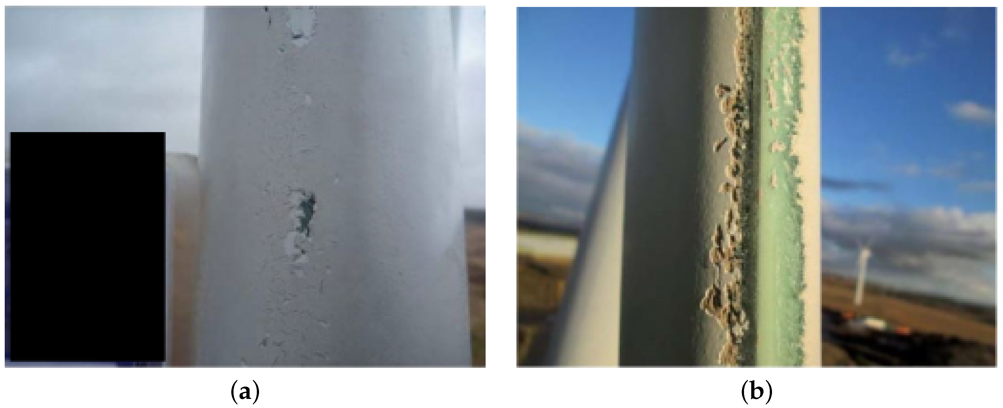

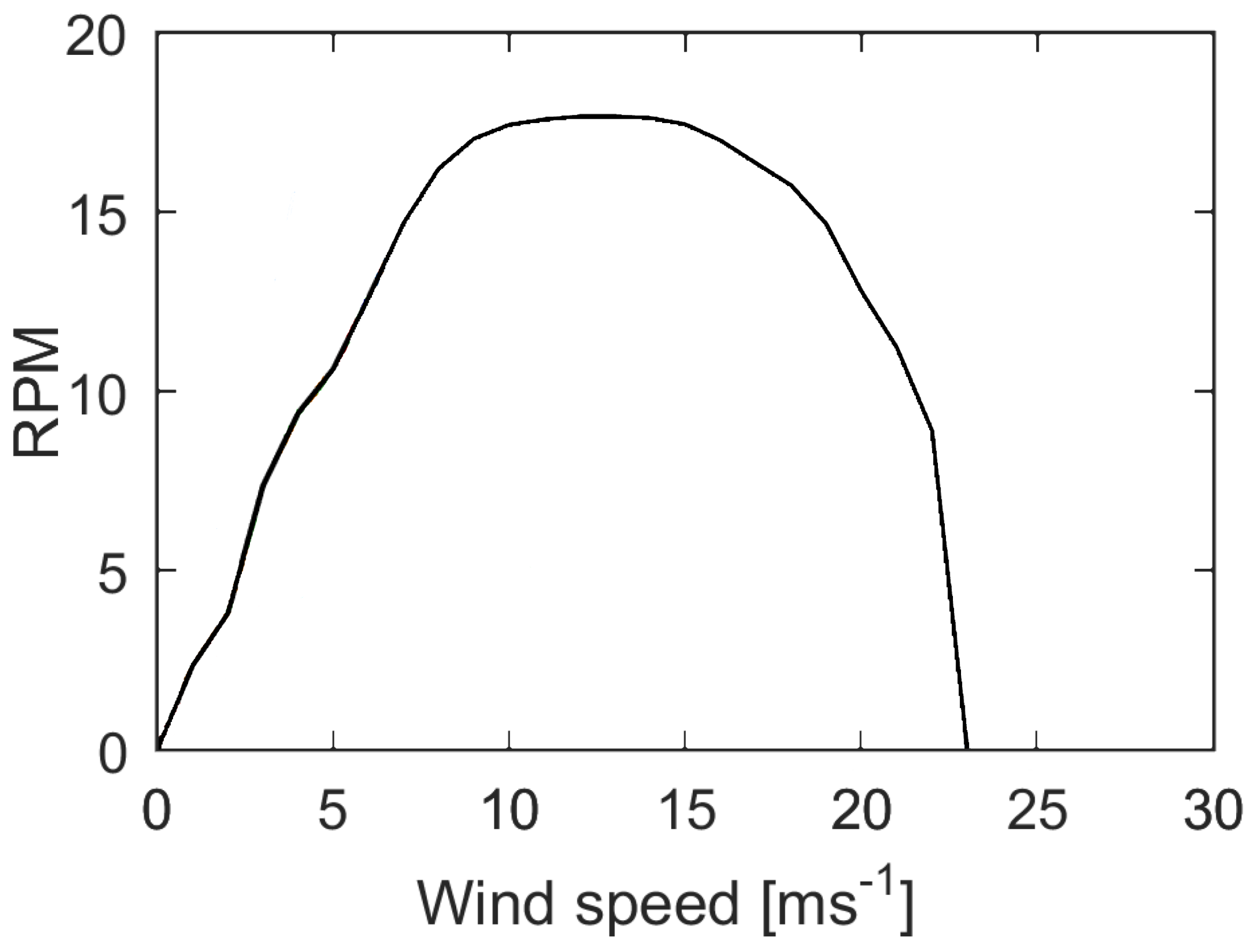
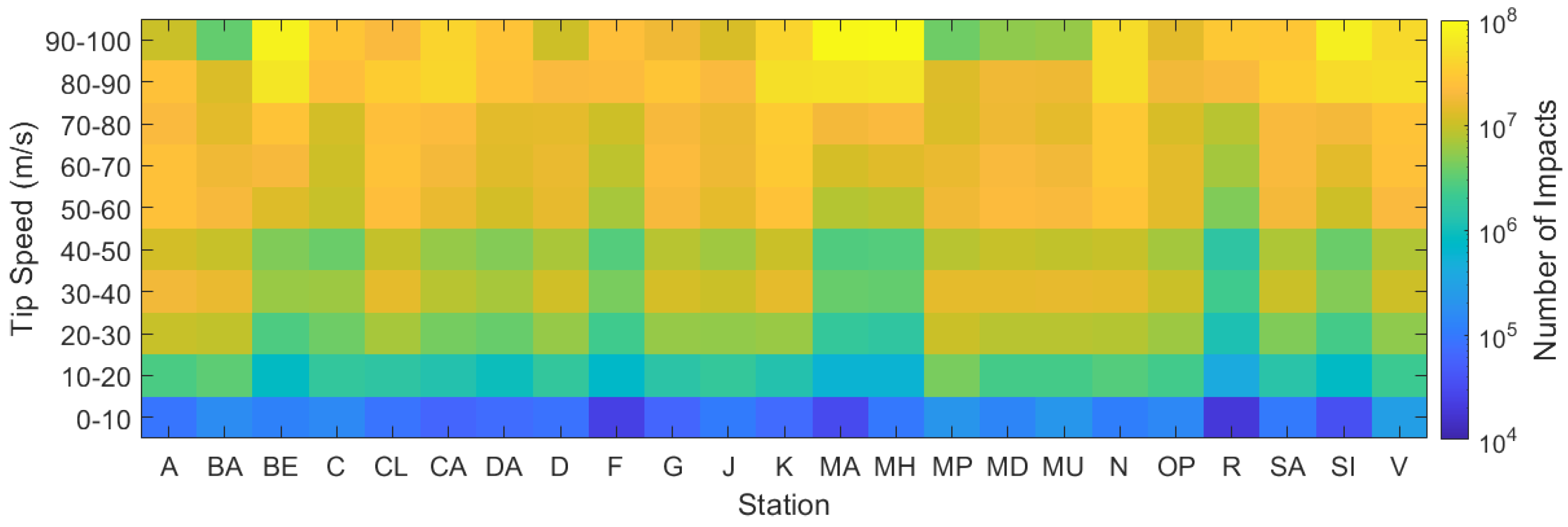
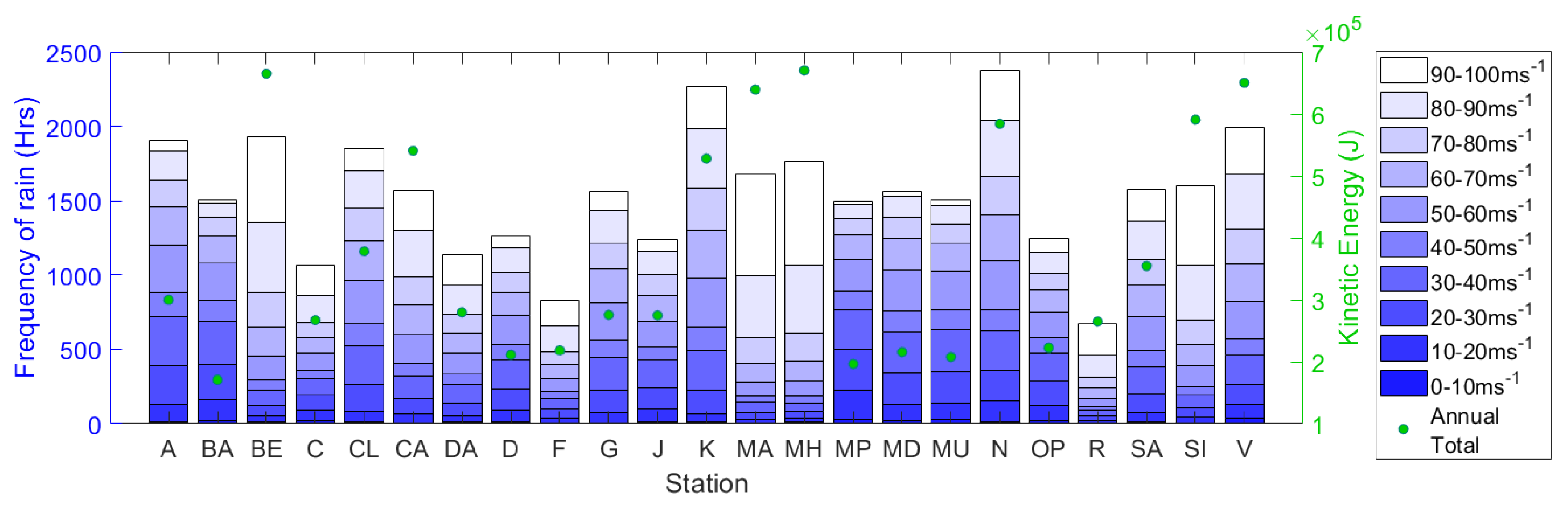
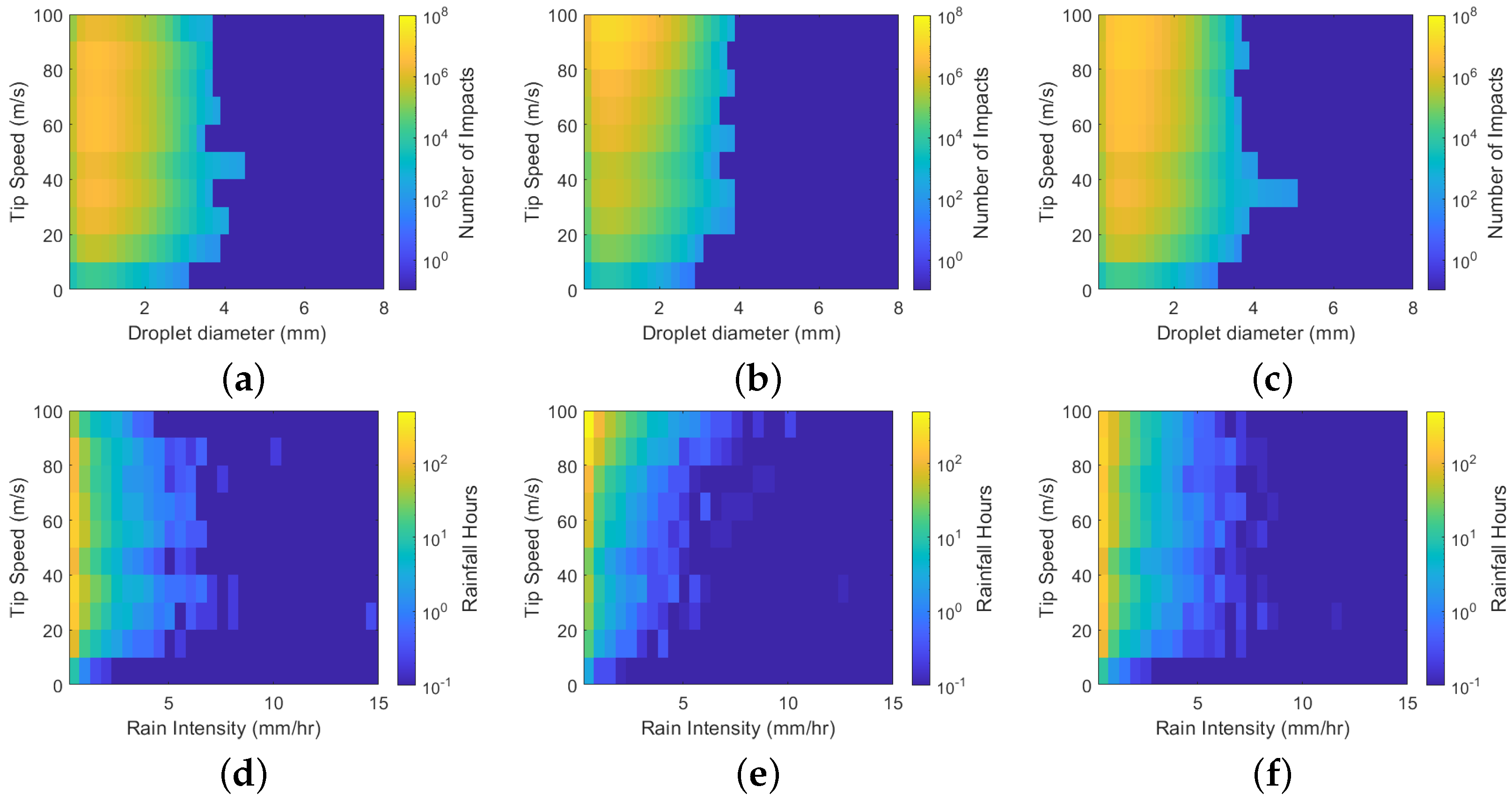
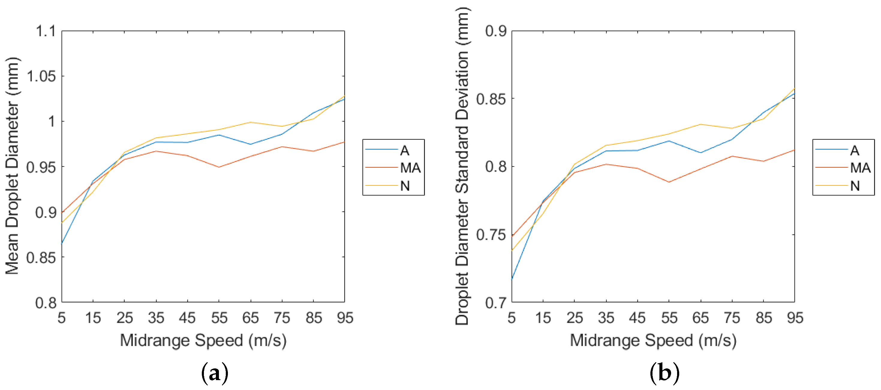
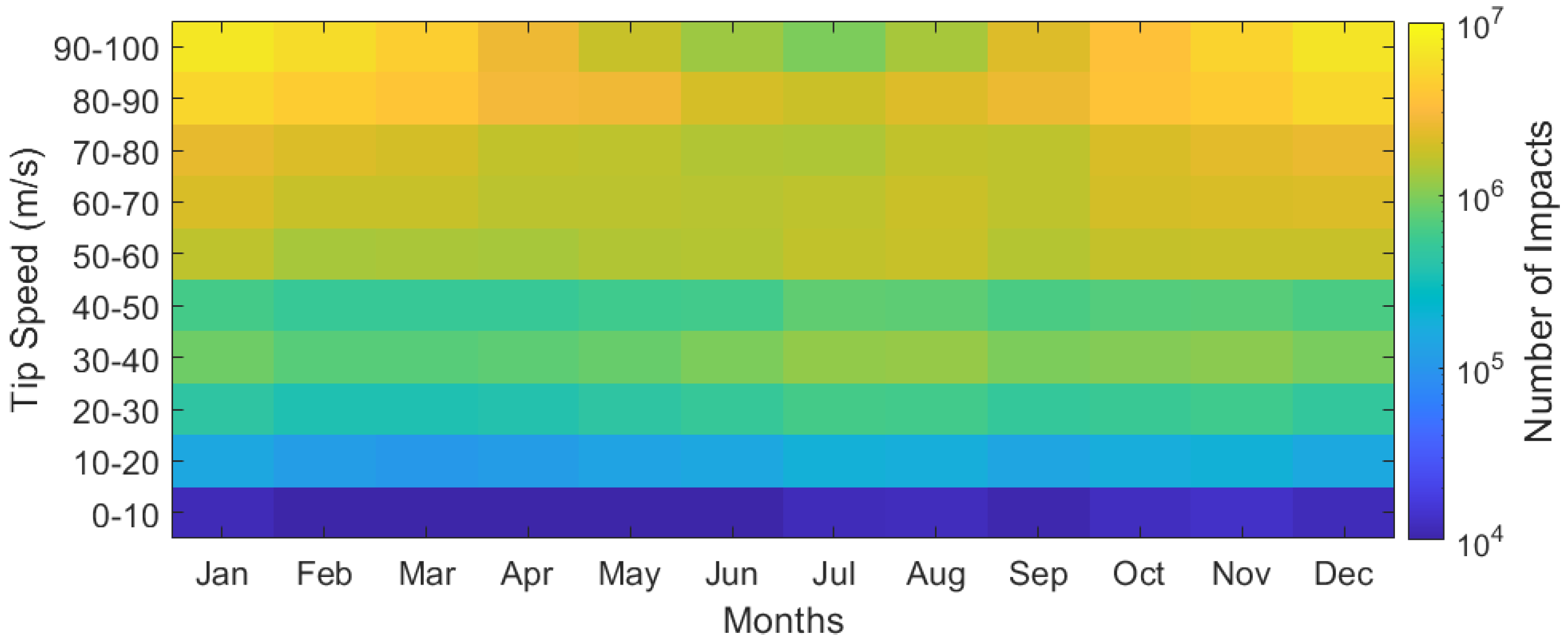
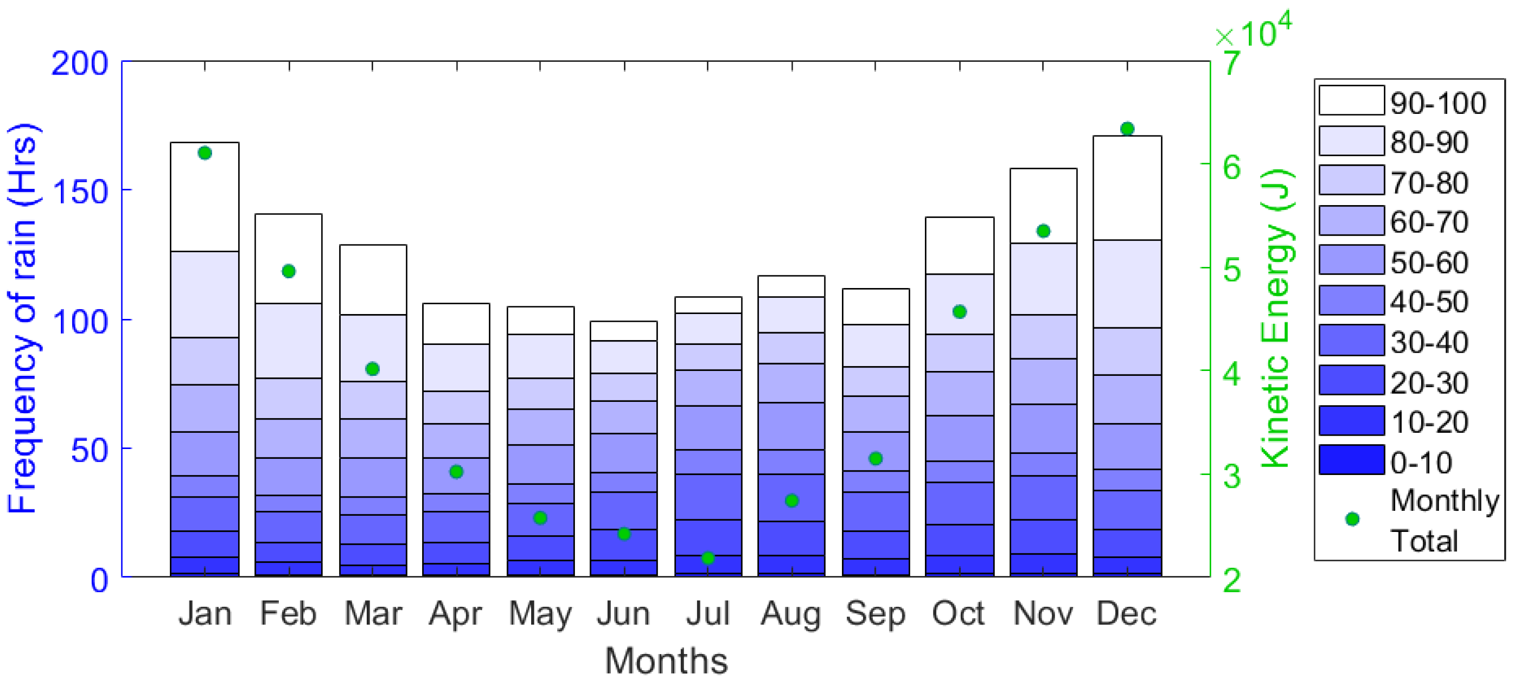
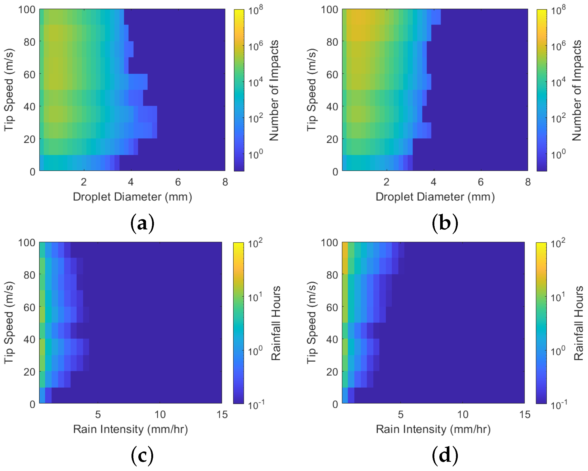
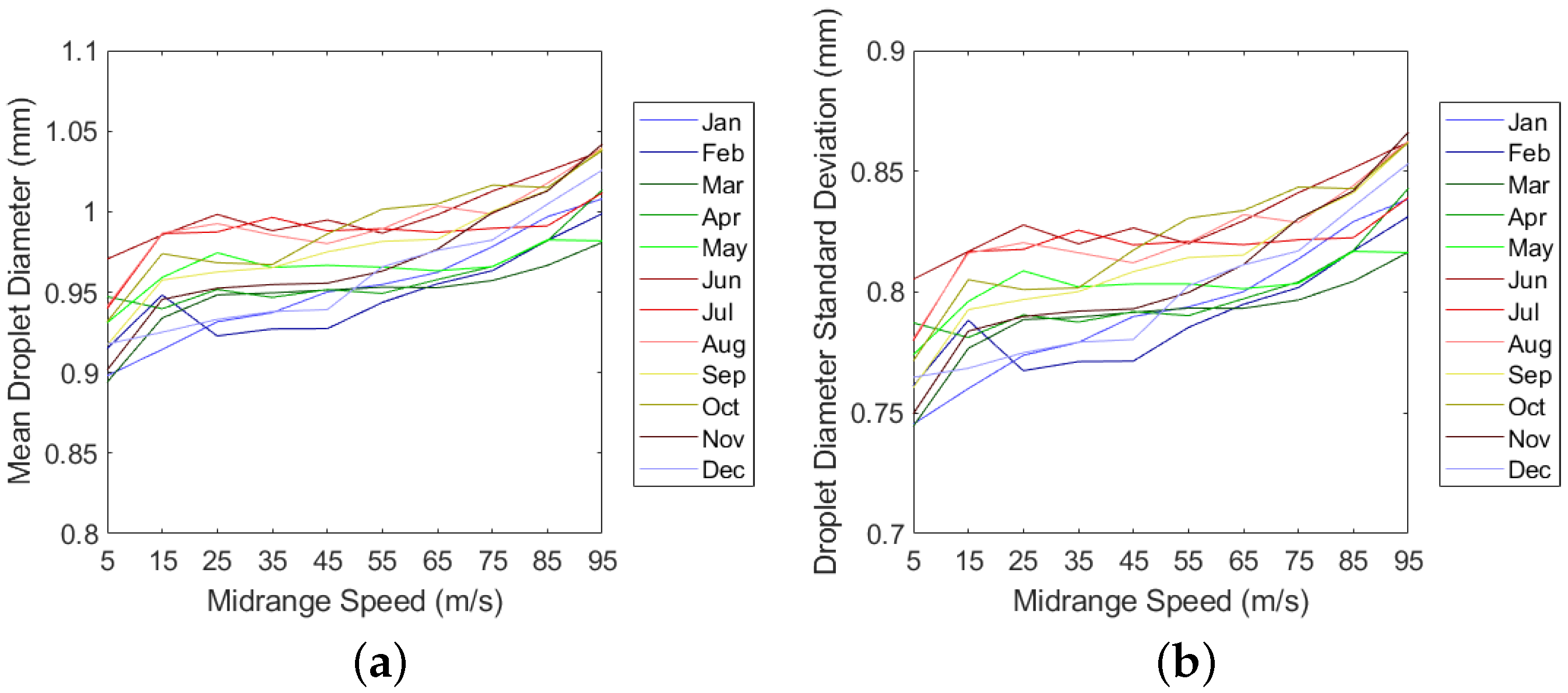
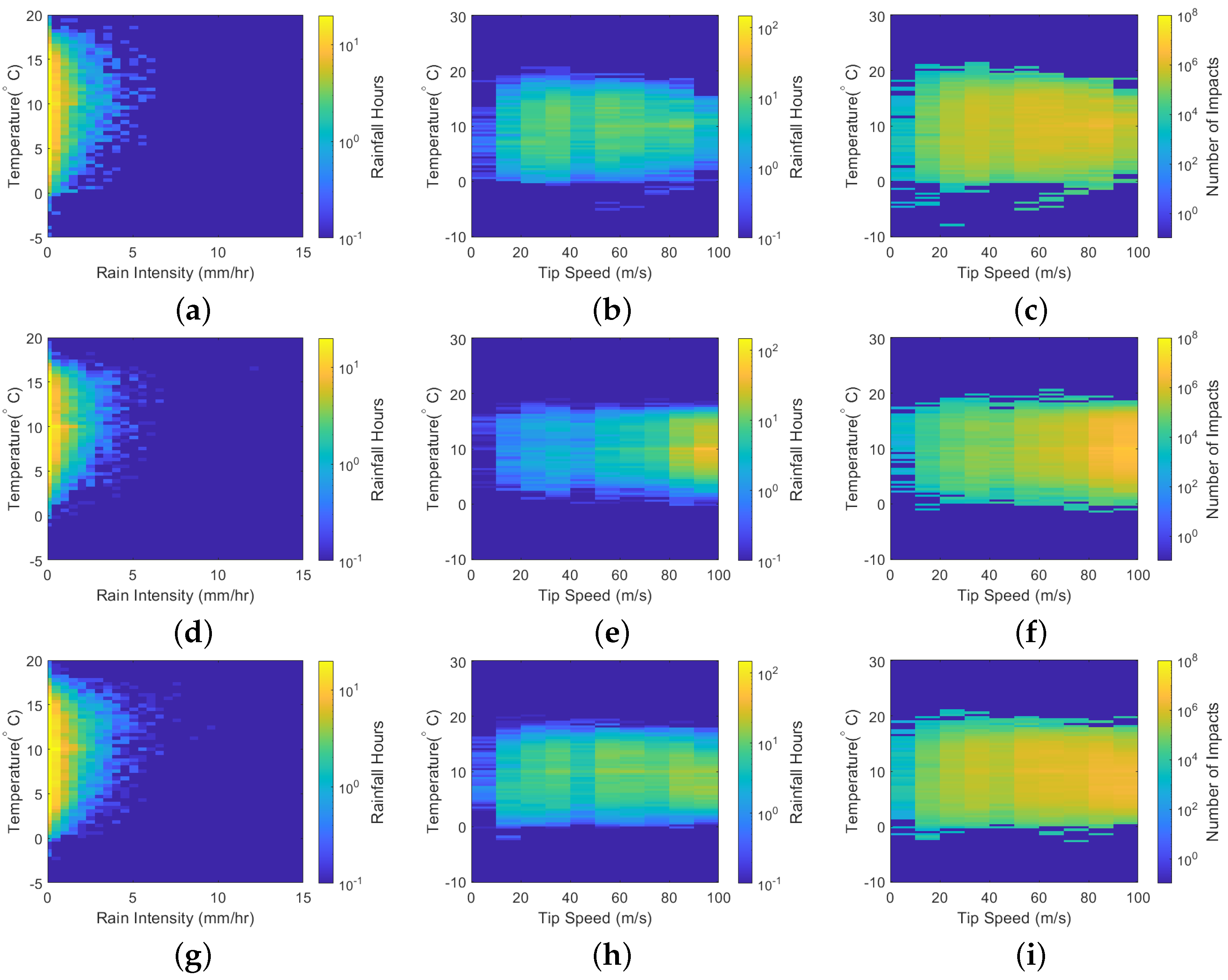

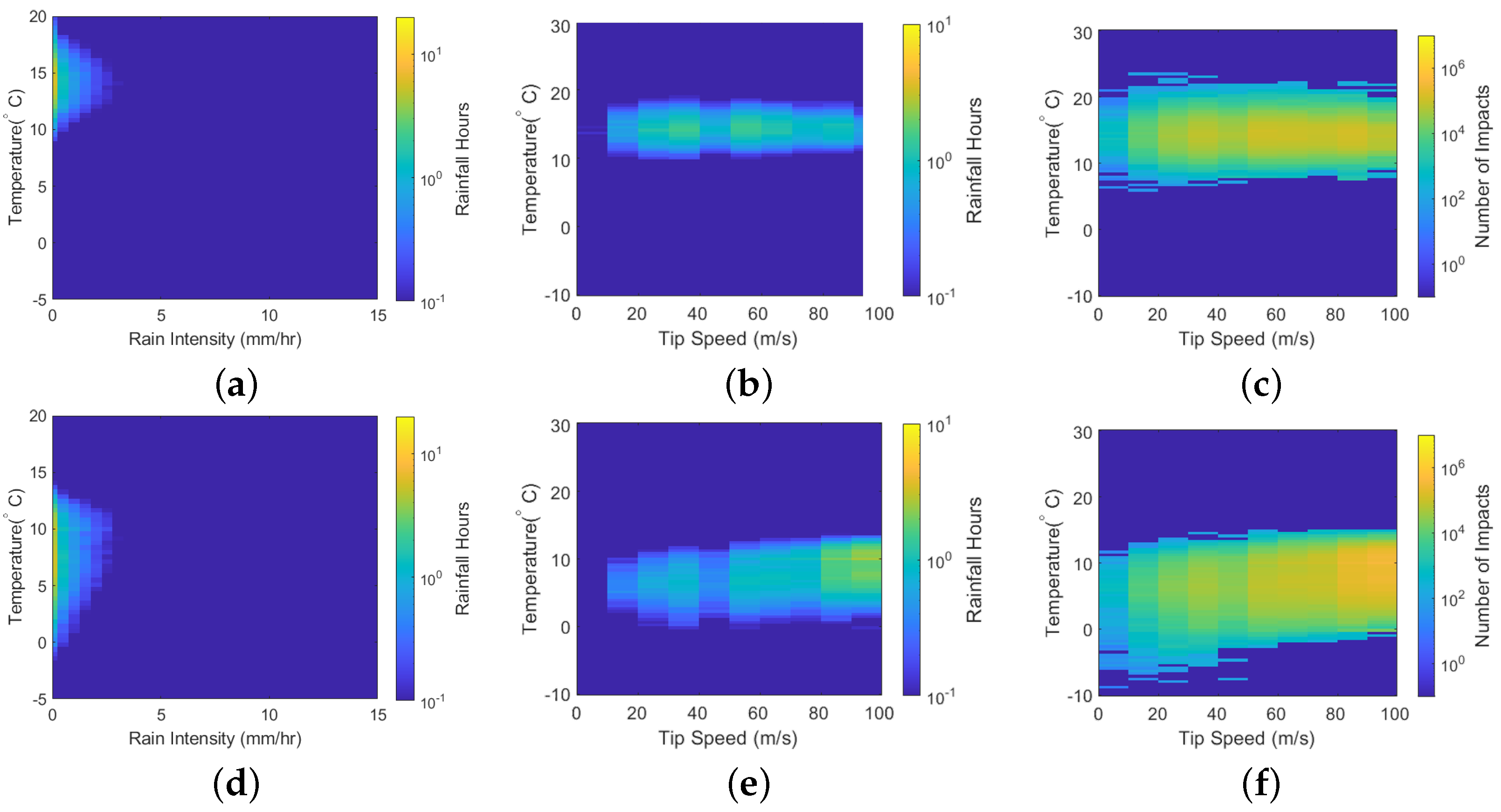
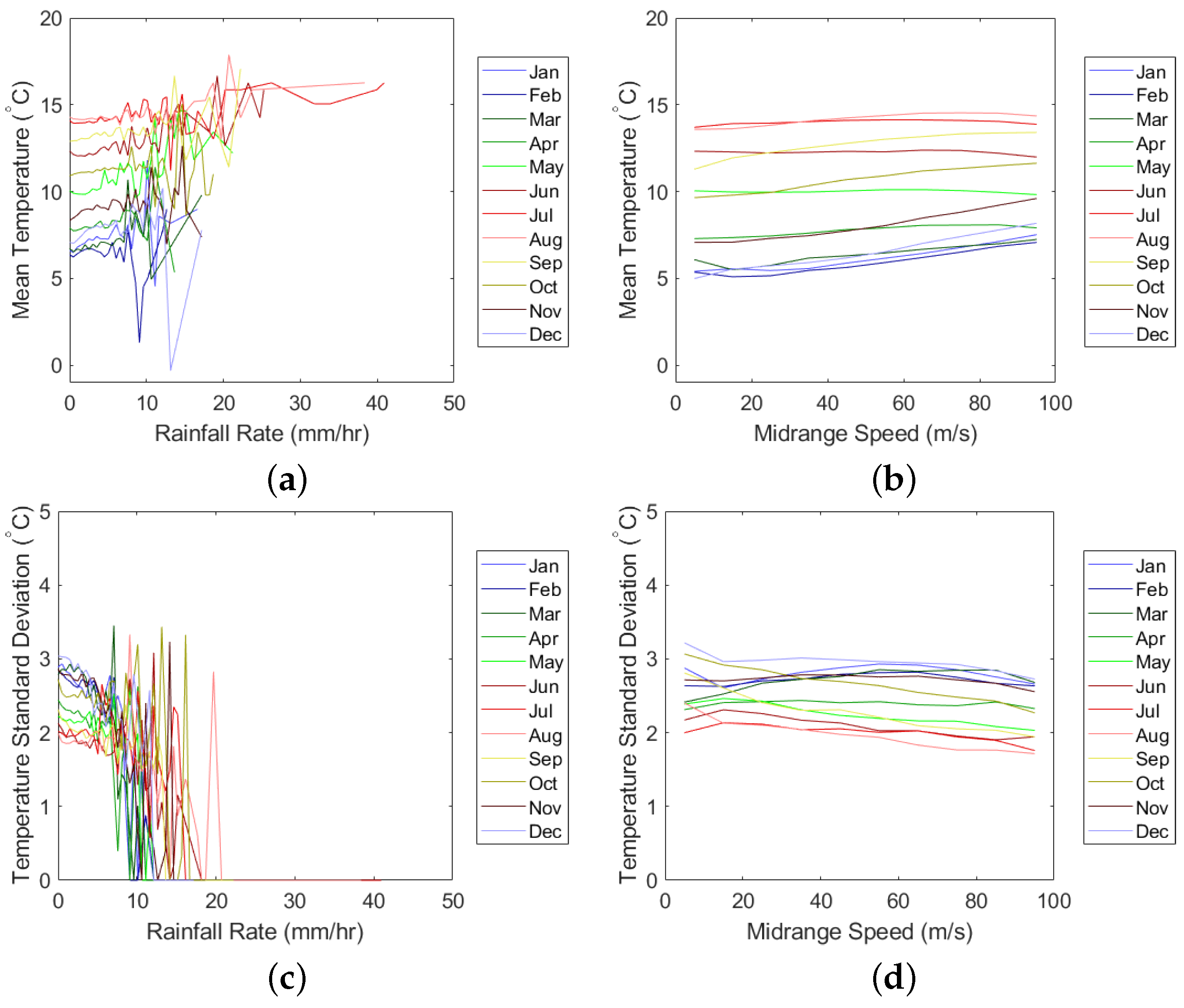
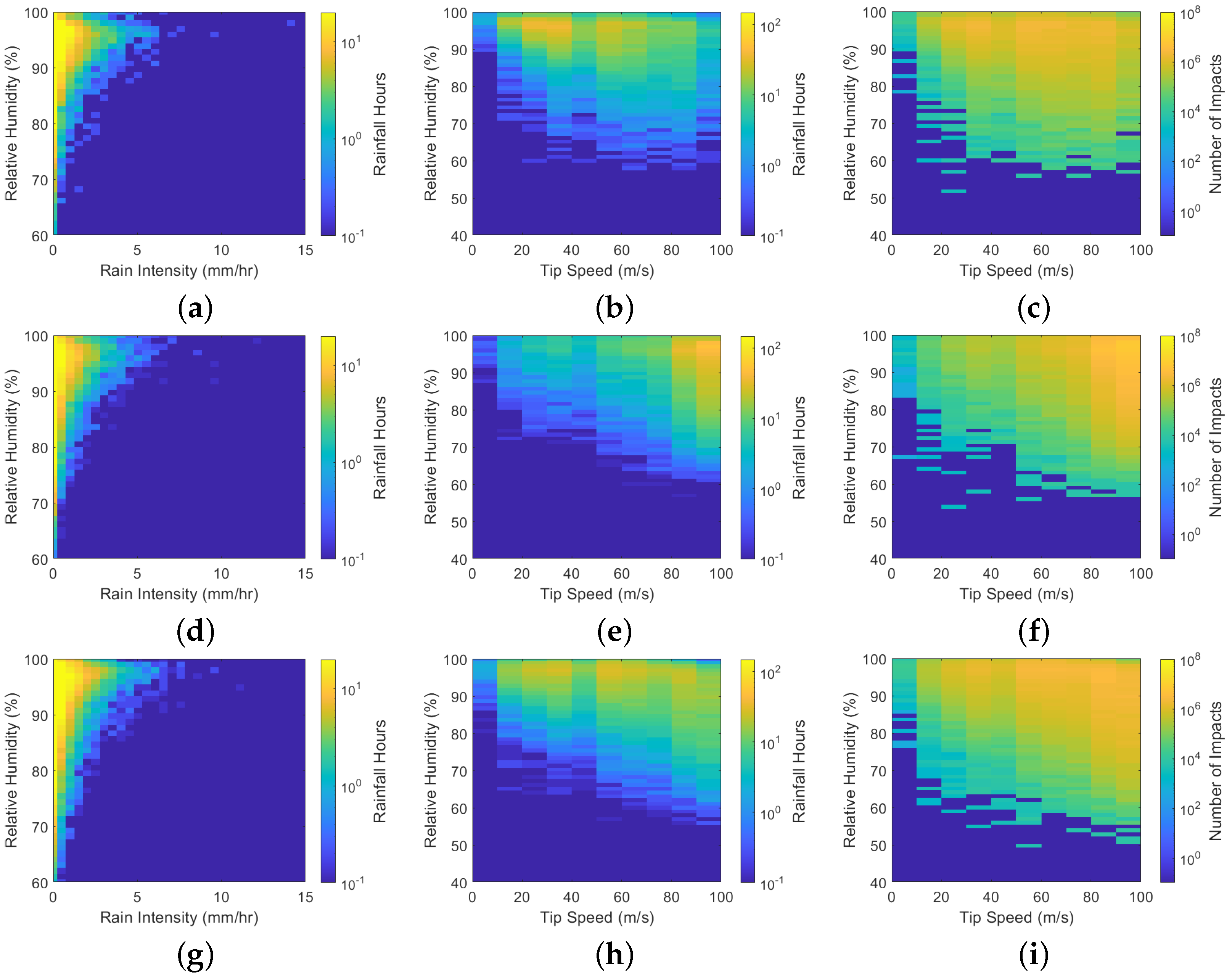
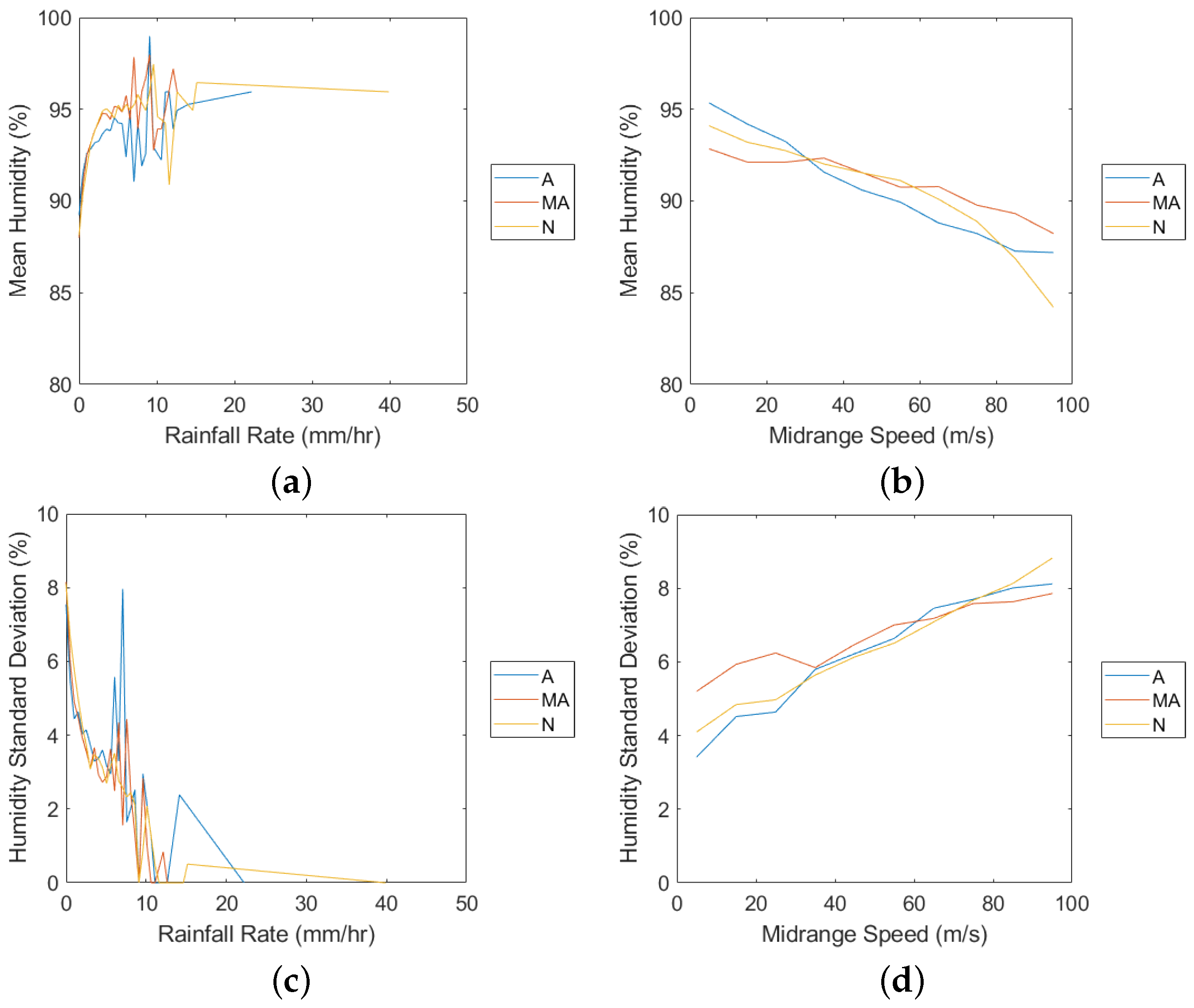
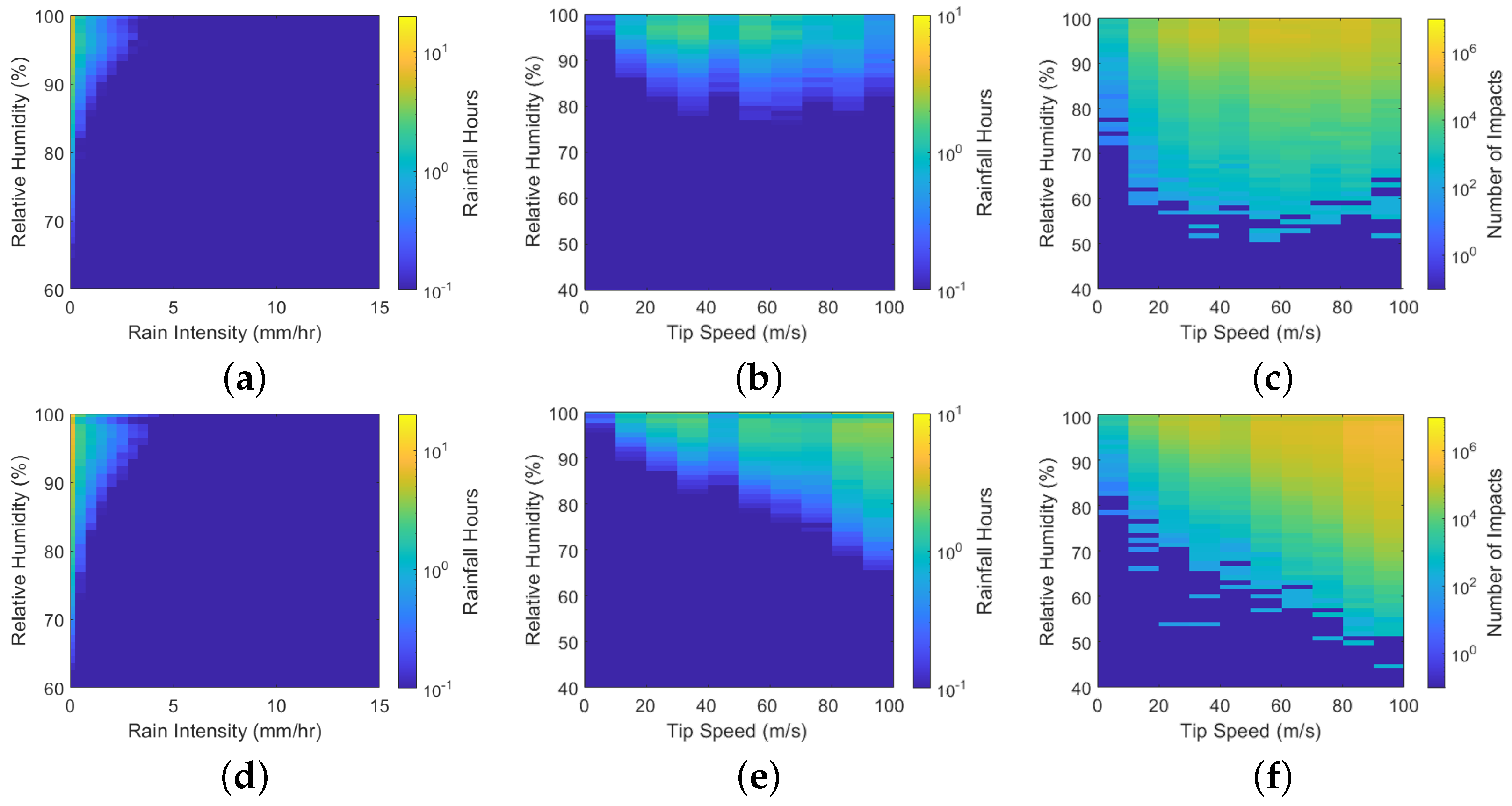

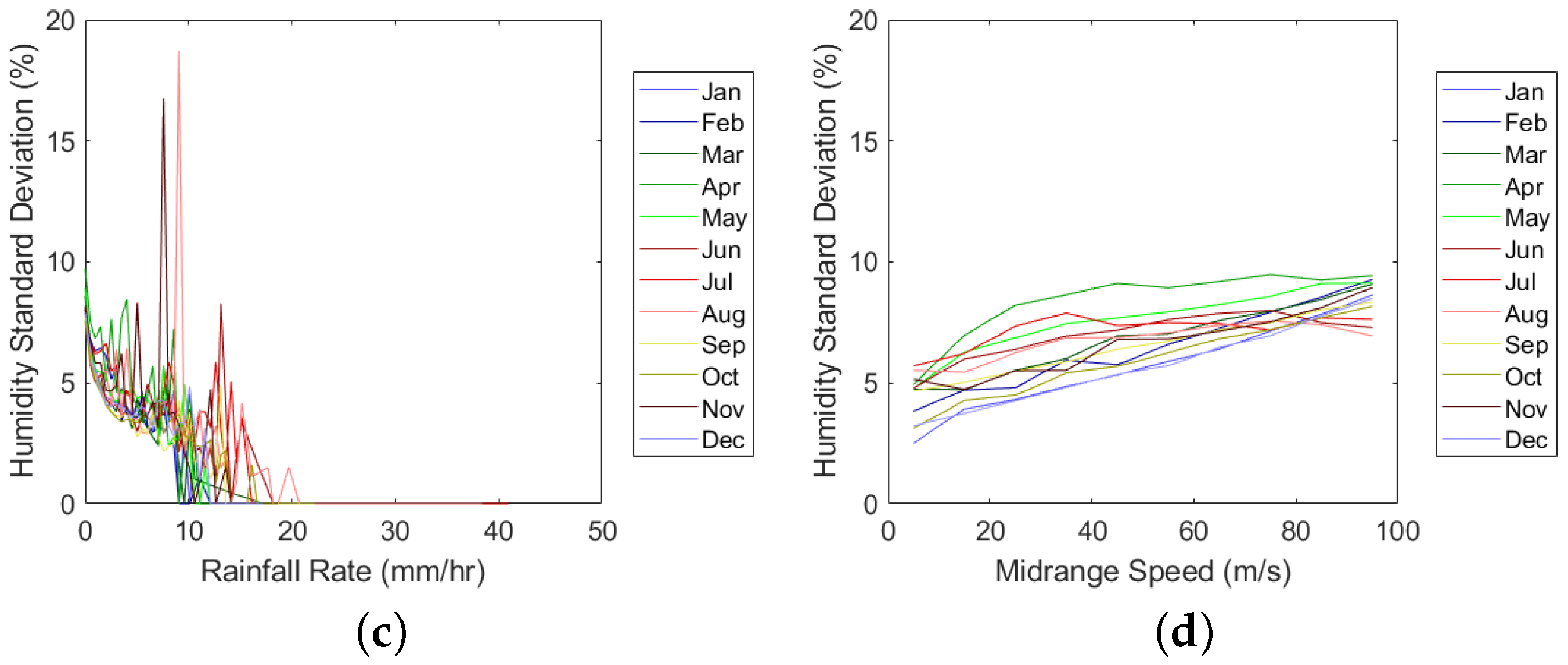
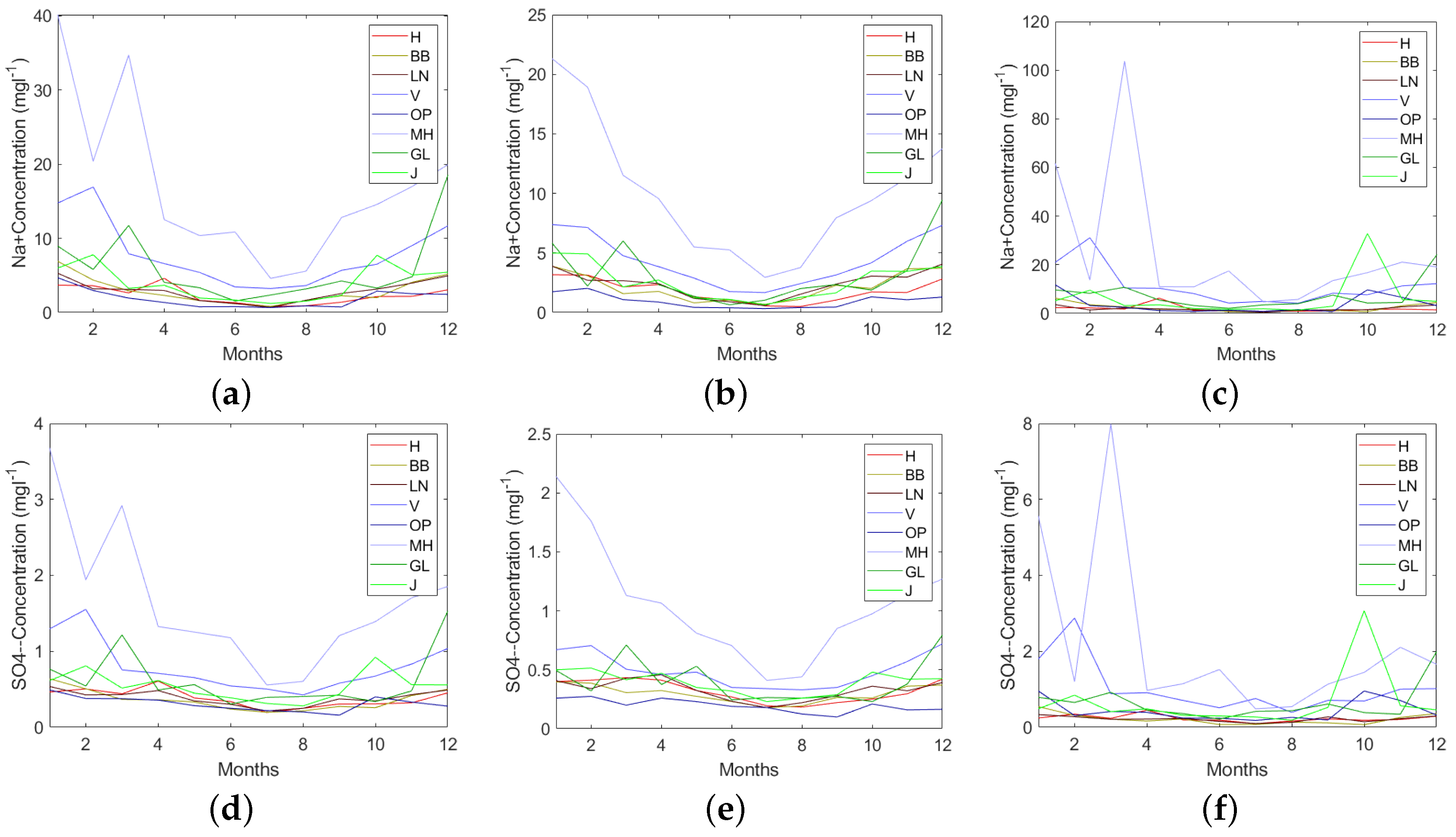
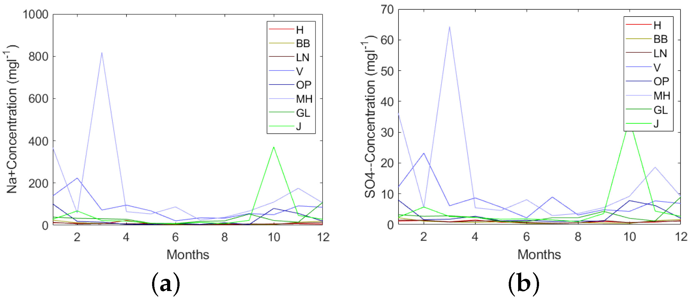

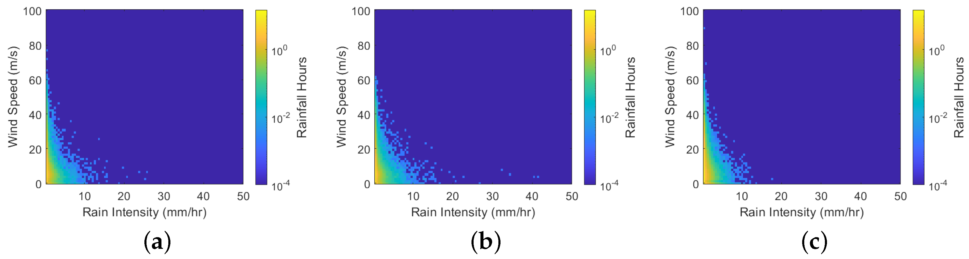

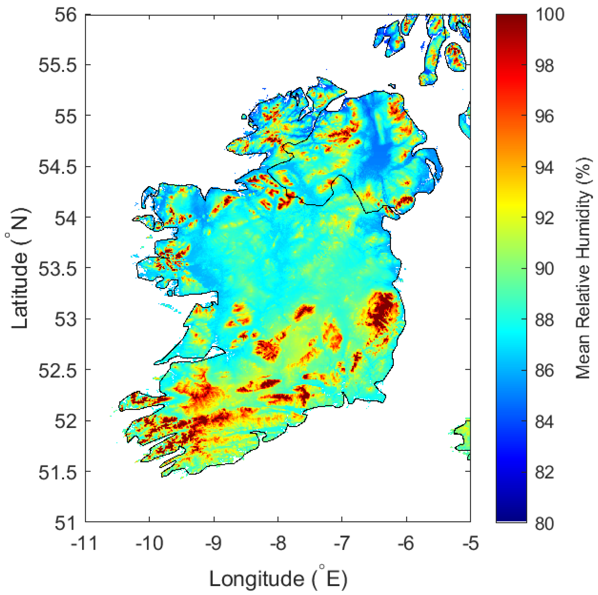
Publisher’s Note: MDPI stays neutral with regard to jurisdictional claims in published maps and institutional affiliations. |
© 2021 by the authors. Licensee MDPI, Basel, Switzerland. This article is an open access article distributed under the terms and conditions of the Creative Commons Attribution (CC BY) license (https://creativecommons.org/licenses/by/4.0/).