The proposed GRASP approach is presented as Algorithm 1.
and
are initialized to ensure the minimum time and the best attained TSP-D solution found so far, respectively. In line 3, the optimal TSP tour is obtained using the Concorde TSP solver. The following steps are repeated
times. The output of
is passed to
, in order to construct an initial TSP-D solution. This is explained in detail in
Section 2.2.1. Following that,
is used to improve the acquired TSP-D solution, which is detailed in
Section 2.2.2.
then computes the cost (objective function) of the current TSP-D solution as
(
Section 2.3). If there are positive savings in cost, with respect to
, the current TSP-D solution is saved as the best solution found thus far,
.
| Algorithm 1: The GRASP algorithm |
- 1
; - 2
; - 3
; - 4
; - 5
while () do - 6
; - 7
; - 8
; - 9
if () then - 10
minTime=currentTime; - 11
bestTour=tspd; - 12
end - 13
; - 14
end - 15
returnbestTour,minTime;
|
2.2.1. Building the Randomized Initial TSP-D Tour
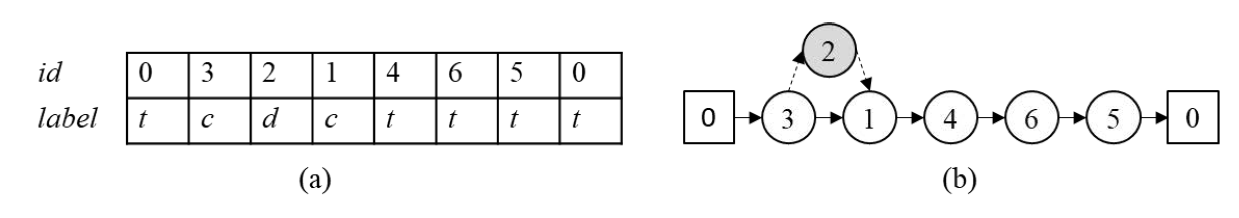
The main function of the initial TSP-D procedure (Algorithm 2) is to perform the initial partitioning of the available truck route into a truck route and a drone route, using the restricted candidate list (RCL).
First, the time saving obtained for all nodes (except the depot) when a node
j is transformed from a truck node to a drone node is computed. The procedure identifies the minimum amount of saved time for all nodes
, the maximum amount of saved time among all nodes
, and an array
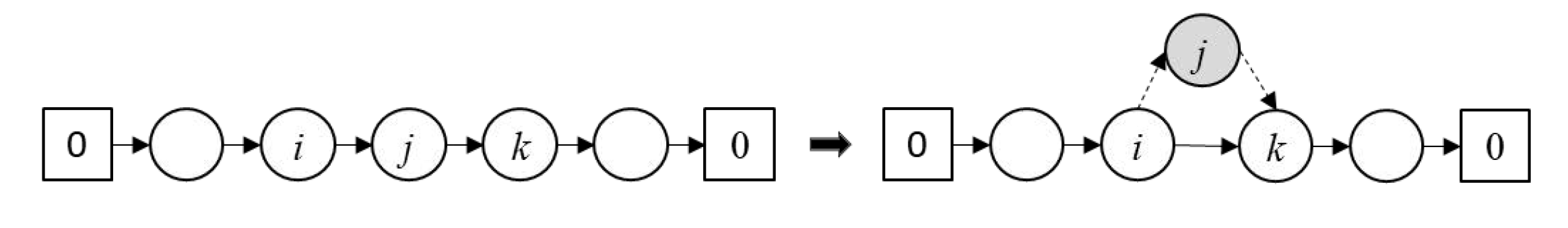
which contains the time saved by each node. The saved time is computed using Equation (
1) and illustrated in
Figure 3, where
i is the node ID of the launch node,
j is the node ID of the drone node, and
k is the node ID of the rendezvous node. Calculating the time savings obtained for all nodes takes
time.
| Algorithm 2: Algorithm |
- 1
; - 2
Generate value, ; - 3
; - 4
; - 5
; - 6
while () do - 7
; - 8
end
|
The threshold value,
, is computed using Equation (
2) [
41], where
is a randomly generated value,
. The RCL is accordingly built by adding the customers that may be serviced by the drone; that is, all nodes
i with
. The
procedure requires
time. Next, nodes are iteratively and randomly selected and removed from the RCL to be transformed into drone nodes, using the
algorithm explained in Algorithm 3.
was inspired by the greedy partitioning heuristic presented by Agatz et al. [
10]. In that method, one of the three moves (
, which converts a truck node to a drone node,
, and
) is randomly selected in each iteration. The selected move is applied to an unprocessed node. However, in this implementation, as presented in Algorithm 3, a candidate node,
, is chosen randomly and removed from the RCL, in order to be converted into a drone node.
can be a drone node if it has a predecessor and a successor, meaning that it is not a boundary node. In addition, it must not lie in a sortie. Once this move is successful, the feasibility of the
and
moves for the sortie under consideration is examined. If both moves can be feasibly implemented while improving the cost, then one of them is greedily selected, such that the cost saving is maximized. Otherwise, the feasible move is applied if it improves the cost.
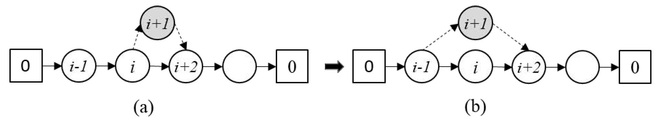
inserts the truck node to the left of the launch node into the sortie, as shown in
Figure 4. The move is only feasible if the node preceding the launch node is a truck node other than the depot and is not part of a sortie. The time taken by the sortie before applying
,
, is calculated using Equation (
3). Equation (
4) computes the time taken by the sortie after applying
,
. The time saved is computed by taking the difference between
and
. If the procedure results in time savings greater than zero, the move is accepted. The
operator is symmetric with respect to
. Converting the
into a drone node in lines 4–10 of Algorithm 3 requires
time. The complexity of both moves, including the work required to compute the savings obtained by the moves, is
time. However, the time required by the
step at line 1 of the algorithm is
(
Section 2.3), resulting in a time of
for
. The
algorithm is called a number of times equal to the length of the RCL as in line 6 from Algorithm 2. Accordingly, the time complexity required by the
algorithm is
.
| Algorithm 3: algorithm |
- 1
; - 2
=randomly select an element from RCL; - 3
Find the position i of in ; - 4
if ( can be a drone node) then - 5
; - 6
; - 7
; - 8
Set labels for nodes , , and to , , and , respectively; - 9
- 10
end - 11
if (both and are feasible) then - 12
Greedily select and apply the move that maximizes cost savings to ; - 13
else - 14
if ( is feasible) then - 15
Apply to ; - 16
else - 17
if ( is feasible) then - 18
Apply to ; - 19
end - 20
end - 21
end - 22
returnRCL, tspd
|
2.2.2. Optimizing the Obtained Solution with Local Search
The LS procedure helps to improve the initial TSP-D solution by applying two different moves:
and
[
10]. The LS procedure is explained, followed by a description of the two moves.
A general structure for the LS procedure is shown in Algorithm 4. After the initialization step, an iterative process starts. In each iteration, either the
or
move is selected in a self-adaptive manner, based on the move probability,
, as follows (lines 7–12). A random number,
, is generated. If the value of
is less than
, the
move is selected; otherwise, the
move is selected. The selected move is applied to the current solution,
. If the resulting neighbor has a lower cost, the move is accepted. Otherwise, the acceptance criterion is tested. The success ratio of the chosen move is updated. The procedure is repeated until the termination condition or
is reached.
| Algorithm 4: Algorithm |
- 1
; - 2
initialize loop control parameters; - 3
while(termination condition not satisfied and ) do - 4
if ( iterations have elapsed) then - 5
update based on Equation ( 5); - 6
end - 7
=generate a random number ; - 8
if () then - 9
apply swap move to and update its success ratio; - 10
else - 11
apply twoOpt move to and update its success ratio; - 12
end - 13
examine move acceptance criteria and accept move accordingly; - 14
if (the move was not successful) then - 15
increment j; - 16
else - 17
reset j; - 18
end - 19
update iteration control parameters; - 20
end
|
The move selection probability,
, is updated consistently after a certain number of iterations,
, based on the success ratio of the
and
moves:
and
, respectively (lines 4–6 in Algorithm 4). The success ratio is computed as the number of times that the move is successfully applied, divided by the total number of times that the move was applied during the past
. If
is better than
,
is updated such that
has a higher probability of being chosen and vice versa, as shown in Equation (
5), where
is a learning rate parameter.
Moreover, in order to control the computational time, the convergence is examined and the LS procedure is stopped if it fails to improve the solution after a specific number of iterations (), as shown in lines 1 and 14–18.
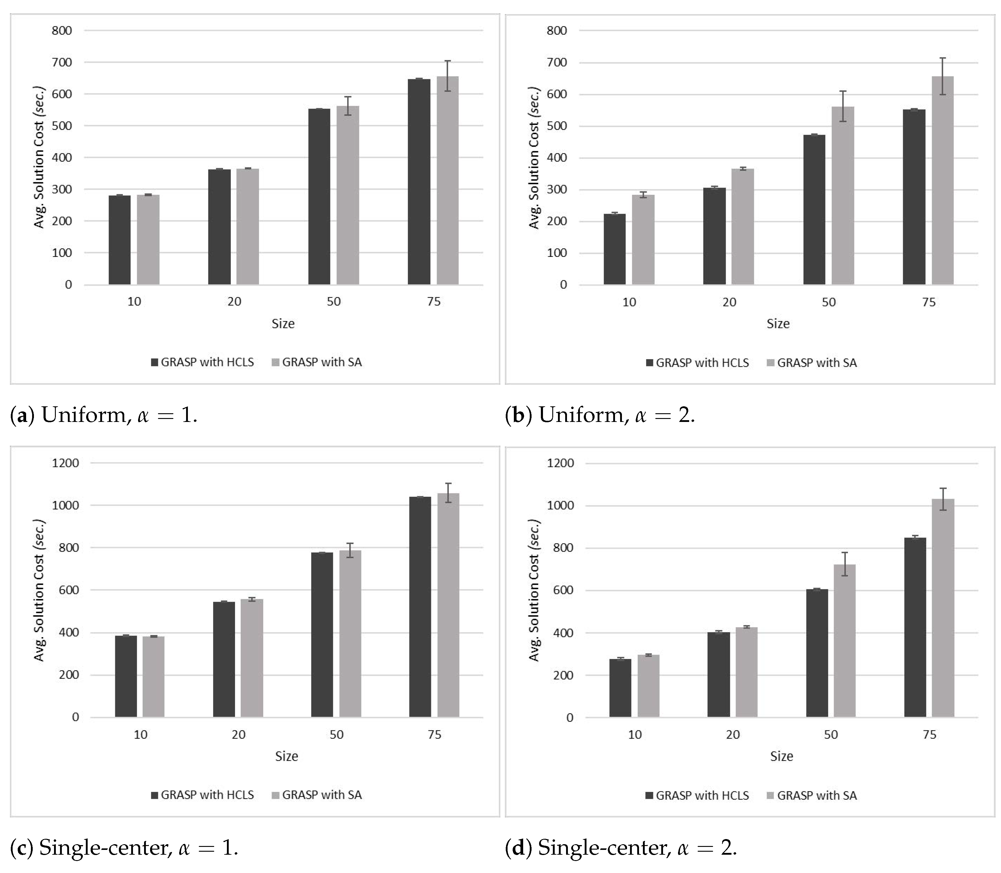
Two variants of GRASP were considered, according to the LS procedure used: hill-climbing local search (HCLS) [
42] and LS with simulated annealing (SA) [
26]. These variants differ in terms of the initialization step and the acceptance criteria (lines 2 and 13 in Algorithm 4, respectively). In the HCLS variant, the loop control parameter is a simple loop counter
i, which is initialized to zero. The termination condition is satisfied when
i reaches the maximum number of allowed iterations,
. In this variant, a move is accepted only if the resulting neighbor has a lower cost than that of the current solution.
In the second variant, SA, the loop is controlled by a temperature parameter,
.
is initialized to an initial temperature,
, and updated using a geometric cooling schedule, as shown in Equation (
6), where
[
26]. The acceptance criterion in SA differs from that in the HCLS variant for inferior moves. A sub-optimal move can be accepted, based on a certain probability
that it follows the Boltzmann distribution, as shown in Equation (
7), where
represents the difference between the objective function (cost) of the current solution and that of the resulting neighbor. A random number,
, is generated. If the value of
is less than the probability
, the move is accepted; otherwise, the move is not accepted. The termination condition in the SA variant is satisfied when the temperature
exceeds the final temperature
.
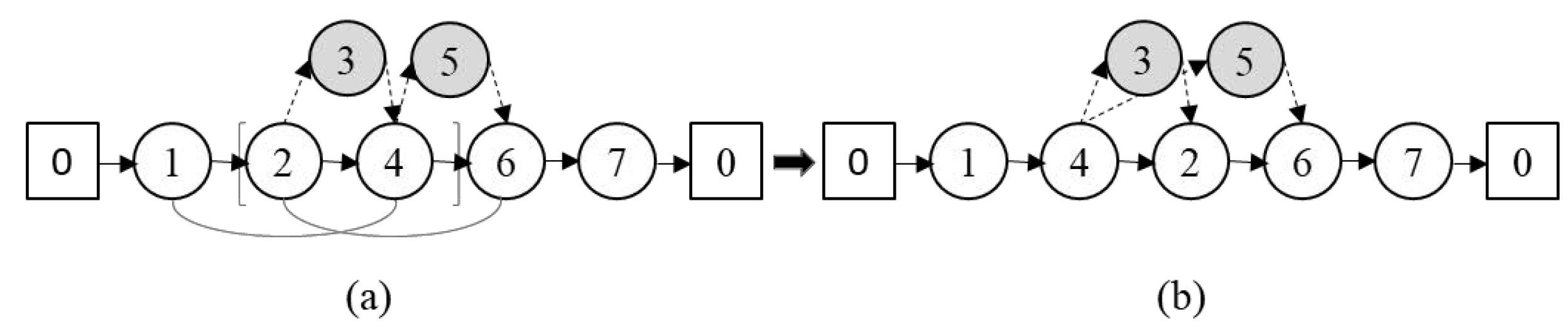
The
Move: In the
move, two distinct nodes are randomly selected and swapped (
Figure 5). A swapped node may be a truck node, a drone node, or a combined node, but it cannot be the depot [
22].
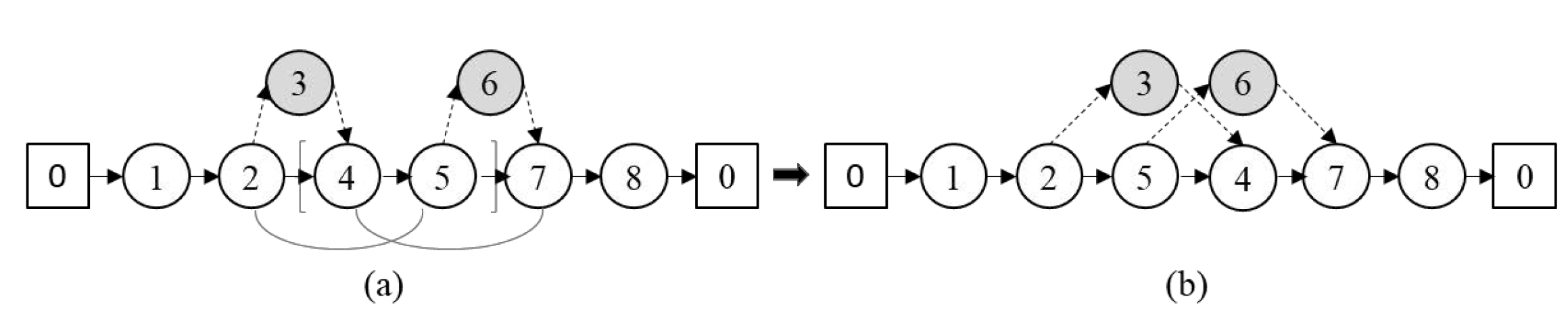
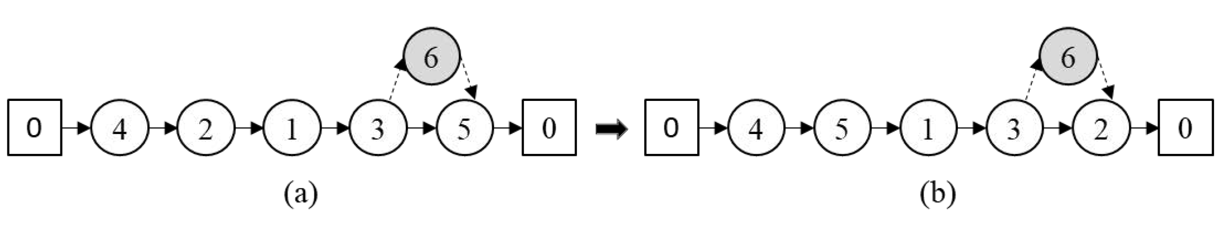
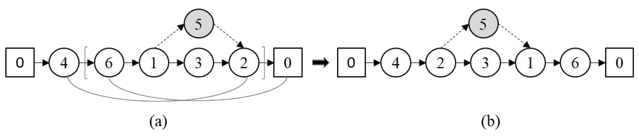
The
Move: In the
move, two edges are removed from the tour and replaced with another set of edges, in order to obtain a valid tour. The removed edges must be between truck or combined nodes [
22]. The first step in applying
is to select the two origin nodes of the selected edges randomly. In
Figure 6a, nodes 4 and 2 are selected. Two edges are thus removed:
and
. Then, two new edges are created, as shown in
Figure 6b:
and
. As a result, the sortie path is reversed, as shown in
Figure 6b.
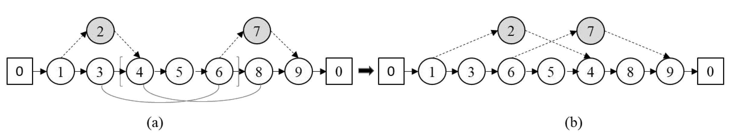
As twoOpt randomly selects two edges, there are several invalid cases that must be taken into consideration, as follows:
- 1.
If the selected origin node or its destination node happen to be inside a sortie, as shown in
Figure 7;
- 2.
If both selected origin nodes are launch nodes and their destinations are rendezvous nodes, as shown in
Figure 8;
- 3.
If the selected origin or its destination node happens to be a common node between different sorties, as shown in
Figure 9.
The complexity of and moves, including the work required to compute the savings obtained by the moves, is .


 ,
, 


