Huanglongbing Model under the Control Strategy of Discontinuous Removal of Infected Trees

Abstract

By using differential equations with discontinuous right-hand sides, a dynamic model for vector-borne infectious disease under the discontinuous removal of infected trees was established after understanding the transmission mechanism of Huanglongbing (HLB) disease in citrus trees. Through calculation, the basic reproductive number of the model can be attained and the properties of the model are discussed. On this basis, the existence and global stability of the calculated equilibria are verified. Moreover, it was found that different $I_0$ in the control strategy cannot change the dynamic properties of HLB disease. However, the lower the value of $I_0$, the fewer HLB-infected citrus trees, which provides a theoretical basis for controlling HLB disease and reducing expenditure.

1. Introduction

Vector-borne disease is an infectious disease spread by media. These diseases do not only occur in the population, but also affect tree populations. Huanglongbing disease is a kind of vector-borne disease in plant populations. As an infectious disease affecting plants, citrus Huanglongbing (HLB) disease results in inestimable profit loss in terms of the production of citrus fruit. Therefore, the disease is regarded as a cancer in the citrus orchard. The transmission of citrus HLB disease has a history of nearly 100 years in China. However, the transmission of the disease was not reported until the early 20th century, when first identified in south China (in Guangdong and Fujian provinces as well as the Guangxi Zhuang autonomous region). During the 1970s and 1980s, citrus HLB disease spread to multiple provinces (including Jiangxi, Yunnan, and Sichuan provinces) in China, affecting the production of citrus fruit and damaging the agricultural economy in local areas. Moreover, the disease tended to spread to surrounding provinces [1]. As expected, among 19 provinces of China where citrus trees were planted, more than two thirds suffered HLB disease after several years. To date, the HLB disease mainly occurs in more than 50 countries and regions in five continents (except for Europe and Antarctica) [2]. Through investigation, Psyllidae is the main transmitting vector of HLB disease, which leads to an extremely rapid rate of transmission. Moreover, with fruit pulp of poor quality, the yield from HLB-infected citrus trees decreases and the longevity of such trees declines. As a result, the citrus industry fails to develop, which leads to a huge economic loss for local agricultural production. To guarantee the normal growth of citrus trees and the increase in profits from agricultural production, it is essential to explore the development of HLB disease and effectively prevent and control it. To date, citrus species have no real resistance to HLB disease, and there is no effective treatment for this disease. Mathematical models play an important role in analyzing the epidemiology of vector-borne plant pathogens. Van der Plank [3] and Kranz [4] first used the mathematical dynamics model to study the dynamics of plant diseases. In 1998, J. Jeger et al. established in the literature [5] the kinetic model of vector transmission of the African cassava mosaic disease with constant coefficients. The HLB model can be established with similar methods. There are currently several HLB mathematical models to analyze how HLB spreads among individual trees, citrus groves, or forests [6]. Chiyaka et al. [7] first proposed a mathematical model to describe and analyze the transmission of HLB in trees, and studied the effect of flushing on the dynamics of psyllids. Vilamiu et al. [8] proposed a model of HLB transmission between citrus plants, including delay time and continuous human intervention.

In recent decades, an integrated management strategy for diseases has become widely used in treating plant diseases: this includes replanting, removing inferior plants, introducing natural enemies, genetic modification, and the spraying of pesticides. At present, numerous scholars have applied an integrated management strategy for diseases to an epidemic dynamics model. In addition, obtaining the solution of a differential equation is an important means to investigate its dynamic behavior. The common methods of approximate analytical solution are: homotopy perturbation method [9,10,11,12,13]; homotopy analysis method [14,15]; variational iteration method [16,17,18]; Taylor series method [19]; etc. [20,21,22]. The impulsive differential equation is the most widely employed, based on which many scholars (for example, Jin Zhen [23], Gao Shujing [24], S.Y. Tang, Y.N. Xiao [25] et al.) have drawn fruitful conclusions. Moreover, Meng and Li [26] discussed a type of infectious disease model for plants under fixed-time pulse removal and planting. The threshold $R_1$ for discriminating the development of the disease was proposed and it showed that the infection-free periodic solution of the system is stable on condition that $R_1<1$; however, for $R_1>1$, the disease will be permanent. Nevertheless, the strategy of implementing planting and fixed-time removal is baseless. For the management of disease, it is necessary to utilize multi-stage control measures according to the degree of infection. The multi-stage control strategy is mathematically discontinuous. Discontinuous power systems existed in large numbers in real life. Due to the limitation of analytical tools, the development of the theory of differential equations with a discontinuous right-hand side is relatively lagging and rather slow. Scholars of the former Soviet Union such as F. Filippov performed a lot of excellent work on this, in the meaning of the solution defined by it, by systematically analyzing the basic properties of the understanding and the stability of the system. At present, the theory of differential equations with discontinuous right-hand side is mainly used in artificial neural network dynamics, fishery dynamics, and infectious disease dynamics. For example, M. Forti and P. Nisti investigated the global stability of neural network models with discontinuous activation functions for the first time [27]. Guo Zhenyuan performed research on autonomous fishery models with discontinuous catches and infectious disease models with discontinuous treatment strategies [28,29]. Therefore, differential equations with discontinuous right-hand sides were employed in the model for HLB disease spread to establish a dynamic model for HLB disease under the control strategy of the discontinuous removal of infected trees.

This paper is broadly organized as follows. First, we establish the model, and then use the right discontinuous differential equation theory to analyze the dynamics of the model—mainly the existence and stability analysis of the disease-free equilibrium point and the endemic equilibrium point. Finally, the model is substituted into reasonable parameters, and the correctness of the above conclusions was verified through numerical simulation.

2. Assumptions and Establishment of the Model

In this paper, a mathematical model of vector infectious disease under the control strategy of discontinuous disease tree removal was established on the basis of existing infectious disease models [30,31]. Citrus trees are divided into susceptible and infected trees, which are recorded as $S_h\left(t\right)$, $I_h\left(t\right)$, respectively. The vector Psyllidae is partitioned into susceptible and infected Psyllidae, which are separately marked as $S_v\left(t\right)$ and $I_v\left(t\right)$, respectively. Moreover, the following assumptions are made:

• The total number of citrus trees remains unchanged, i.e., $S_h\left(t\right)+I_h\left(t\right)=K$. If plants are dead, the same number of susceptible citrus trees are re-planted;
• Only Psyllidae which sucks the tender bud of infected citrus trees is regarded as infectious Psyllidae. The susceptible citrus trees which are sucked by infected Psyllidae are considered infected;
• All newly planted citrus trees and new Psyllidae are not infected with HLB disease;
• HLB virus cannot be detected in susceptible citrus trees immediately after infection by Psyllidae but requires a certain time $\tau$ after sucking. The citrus trees are only infectious in this case;
• The reproduction of Psyllidae is controlled by spraying pesticide to control the transmission of citrus HLB disease.

According to the aforementioned assumptions, the following dynamic models are established:

$$\left\{\begin{array}{cc}\hfill \frac{d{S}_h\left(t\right)}{dt}=& C\left(I_h\left(t\right)\right)I_h\left(t\right)+\left({\mu }_1+{\mu }_2\right)I_h\left(t\right)-{\beta }_1{S}_h\left(t\right)I_v\left(t\right)\hfill \\ \hfill \frac{d{I}_h\left(t\right)}{dt}=& {\beta }_1{S}_h\left(t\right)I_v\left(t\right)-\left({\mu }_1+{\mu }_2\right)I_h\left(t\right)-C\left(I_h\left(t\right)\right)I_h\left(t\right)\hfill \\ \hfill \frac{d{S}_v\left(t\right)}{dt}=& \Lambda -{\beta }_2{S}_v\left(t\right)I_h\left(t\right)-d{S}_v\left(t\right)-p{S}_v\left(t\right)\hfill \\ \hfill \frac{d{I}_v\left(t\right)}{dt}=& {\beta }_2{S}_v\left(t\right)I_h\left(t\right)-d{I}_v\left(t\right)-p{I}_v\left(t\right)\hfill \end{array}\right.$$

(1)

where $\Lambda$ represents the constant input rate of susceptible Psyllidae; ${\beta }_1$ and ${\beta }_2$ denote the infection rates of susceptible citrus trees and Psyllidae; ${\mu }_1$ and ${\mu }_1$ represent the natural mortality rate and mortality rate due to disease in citrus trees, respectively; d, p, and $C{I}_h$ denote the natural mortality rate of Psyllidae, the delousing rate arising from the use of pesticide, and the rate of removal of infected trees, respectively; $C{I}_h$ is a piecewise function of $I_h$, such that:

$$C\left(I_h\left(t\right)\right)=\left\{\begin{array}{cc}\hfill c_1,& I_h<I_0\hfill \\ \hfill c_2,& I_h\ge I_0\hfill \end{array}\right.,$$

where $c_1<c_2$.

According to practical biological meaning, it is supposed that all of the aforementioned parameters are positive.

It is noted that $\Omega =\left\{\left.\left(S_h,I_h,S_v,I_v\right)\in R_{+}^4\right|S_h\ge 0,I_h\ge 0,S_v\ge 0,I_v\ge 0\right\}$. In this context, it can be verified that $\Omega$ is a positive invariant set in model (1). Given that $N_v\left(t\right)=S_v\left(t\right)+I_v\left(t\right)$, by adding the third and the fourth equations in system (1), we have:

$$\frac{d{N}_v}{dt}=\Lambda -\left(d+p\right)N_v,$$

Accordingly, $\underset{t\to +\infty }{lim}{N}_v\left(t\right)=\frac{\Lambda }{d+p}\stackrel{\Delta }{=}{N}^{*}$ is reached. The model is mainly to explore the changing trend of diseased citrus and diseased psyllids. Because of $N_v\left(t\right)=S_v\left(t\right)+I_v\left(t\right)$, $\underset{t\to +\infty }{lim}{N}_v\left(t\right)=\frac{\Lambda }{d+p}\stackrel{\Delta }{=}{N}^{*}$ and $S_h\left(t\right)+I_h\left(t\right)=K$, the changes of diseased citrus and diseased psyllids in the system (1) will become more and more similar to the following model over time:

$$\left\{\begin{array}{cc}\hfill \frac{d{I}_h\left(t\right)}{dt}=& {\beta }_1{I}_v\left(t\right)\left[K-I_h\left(t\right)\right]-\left({\mu }_1+{\mu }_2\right)I_h\left(t\right)-C\left(I_h\left(t\right)\right)I_h\left(t\right)\hfill \\ \hfill \frac{d{I}_v\left(t\right)}{dt}=& {\beta }_2{I}_h\left(t\right)\left[N^{*}-I_v\left(t\right)\right]-\left(d+p\right)I_v\left(t\right).\hfill \end{array}\right.$$

(2)

Based on the published literature [32], the solution to model (2) under Filippov conditions can be defined as thus: the vector function $\left(I_h\left(t\right),I_v\left(t\right)\right)$ satisfies the following conditions:

• $\left(I_h\left(t\right),I_v\left(t\right)\right)$ is absolutely continuous in any sub-interval $\left[t_1,t_2\right]$ within $t\in \left[0,+\infty \right)$;
• $I_h\left(0\right)={I_h}_0\ge 0$ and $I_v\left(0\right)={I_v}_0\ge 0$;
• For almost all $t\in \left[0,+\infty \right)$, $\left(I_h\left(t\right),I_v\left(t\right)\right)$ shows the following differential inclusions:

$$\left\{\begin{array}{cc}\hfill \frac{d{I}_h\left(t\right)}{dt}\in & {\beta }_1{I}_v\left(t\right)\left[K-I_h\left(t\right)\right]-\left({\mu }_1+{\mu }_2\right)I_h\left(t\right)-\overline{co}\left[C\left(I_h\left(t\right)\right)\right]I_h\left(t\right)\hfill \\ \hfill \frac{d{I}_v\left(t\right)}{dt}=& {\beta }_2{I}_h\left(t\right)\left[N^{*}-I_v\left(t\right)\right]-\left(d+p\right)I_v\left(t\right)\hfill \end{array}\right.$$

(3)

where $\overline{co}\left[C\left(I_h\right)\right]=\left[C\left(I{}_h^{-}\right),C\left(I{}_h^{+}\right)\right]$:

$$\overline{co}\left[C\left(I_h\left(t\right)\right)\right]=\left\{\begin{array}{cc}\hfill c_1,& I_h<I_0,\hfill \\ \hfill [c_1,c_2],& I_h=I_0,\hfill \\ \hfill c_2,& I_h>I_0.\hfill \end{array}\right.$$

Thus, $\left(I_h\left(t\right),I_v\left(t\right)\right)$ represents the solution to model (2) meeting the initial conditions $I_h\left(0\right)={I_h}_0$ and $I_v\left(0\right)={I_v}_0$ under Filippov conditions.

It can be shown that $(I_h,I_v)\to ({\beta }_1{I}_v\left(t\right)\left[K-I_h\left(t\right)\right]-\left({\mu }_1+{\mu }_2\right)I_h\left(t\right)-\overline{co}\left[C\left(I_h\left(t\right)\right)\right],$ ${\beta }_2{I}_h\left(t\right)[N^{*}-I_v\left(t\right)]-\left(d+p\right)I_v\left(t\right))$ is an upper semi-continuous set-valued mapping with a non-void compact convex set. Before conducting the dynamic analysis of the model, it is shown that model (2) satisfies a positive initial condition $I_h\left(0\right)={I_h}_0\ge 0$. The solution to $I_v\left(0\right)={I_v}_0\ge 0$ shows positivity and boundedness, satisfying biological significance criteria.

3. Dynamic Analysis of the Model

3.1. Existence of Equilibria

Due to the piecewise linearity of control function $C\left(I_h\right)$, the phase plane of $\left(I_h\left(t\right),I_v\left(t\right)\right)$ is divided into three parts:

$$\Sigma =\left\{\left.\left(I_h,I_v\right)\in R_{+}^2\right|I=I_0\right\},G^{-}=\left\{\left.\left(I_h,I_v\right)\in R_{+}^2\right|I<I_0\right\},G^{+}=\left\{\left.\left(I_h,I_v\right)\in R_{+}^2\right|I>I_0\right\}.$$

Therefore, model (2) is expressed as follows within the range of $G^{-}$:

$$I:\left\{\begin{array}{cc}\hfill \frac{d{I}_h\left(t\right)}{dt}=& {\beta }_1{I}_v\left(t\right)\left[K-I_h\left(t\right)\right]-\left({\mu }_1+{\mu }_2\right)I_h\left(t\right)-c_1{I}_h\left(t\right),\hfill \\ \hfill \frac{d{I}_v\left(t\right)}{dt}=& {\beta }_2{I}_h\left(t\right)\left[N^{*}-I_v\left(t\right)\right]-\left(d+p\right)I_v\left(t\right).\hfill \end{array}\right.$$

Within the range of $G^{+}$, it is as follows:

$$II:\left\{\begin{array}{cc}\hfill \frac{d{I}_h\left(t\right)}{dt}=& {\beta }_1{I}_v\left(t\right)\left[K-I_h\left(t\right)\right]-\left({\mu }_1+{\mu }_2\right)I_h\left(t\right)-c_2{I}_h\left(t\right),\hfill \\ \hfill \frac{d{I}_v\left(t\right)}{dt}=& {\beta }_2{I}_h\left(t\right)\left[N^{*}-I_v\left(t\right)\right]-\left(d+p\right)I_v\left(t\right).\hfill \end{array}\right.$$

Within the range of $\Sigma$, it is written as follows:

$$III:\left\{\begin{array}{cc}\hfill \frac{d{I}_h\left(t\right)}{dt}\in & {\beta }_1{I}_v\left(t\right)\left[K-I_h\left(t\right)\right]-\left({\mu }_1+{\mu }_2\right)I_h\left(t\right)-\overline{co}\left[C\left(I_h\left(t\right)\right)\right]I_h\left(t\right),\hfill \\ \hfill \frac{d{I}_v\left(t\right)}{dt}=& {\beta }_2{I}_h\left(t\right)\left[N^{*}-I_v\left(t\right)\right]-\left(d+p\right)I_v\left(t\right).\hfill \end{array}\right.$$

Let the right-hand side of the equation in system I be equal to zero: through calculation, the solution $I_h\left(t\right)\equiv 0$ and $I_v\left(t\right)\equiv 0$ is obtained, i.e., the disease-free equilibrium $E_0=(0,0,)$ of system I. Afterwards, system I is subjected to linearization at the disease-free equilibrium $E_0=(0,0,)$. In this case:

$$\left\{\begin{array}{cc}\hfill \frac{d{I}_h\left(t\right)}{dt}=& {\beta }_{1}K{I}_v\left(t\right)-\left({\mu }_1+{\mu }_2+c_1\right)I_h\left(t\right),\hfill \\ \hfill \frac{d{I}_v\left(t\right)}{dt}=& {\beta }_2{N}^{*}{I}_h\left(t\right)-\left(d+p\right)I_v\left(t\right).\hfill \end{array}\right.$$

According to other work [33], the basic reproductive number $R_1$ of the system I can be calculated, with the following specific steps:

It is defined that $I_{h0}$, $I_{v0}$ separately refer to the initial values of two infected classes $I_h\left(t\right),I_v\left(t\right)$ at $=0$. On this condition, $I_h\left(t\right)=I_{h0}{e}^{-\left({\mu }_1+{\mu }_2+c_1\right)t}$ and $I_v\left(t\right)=I_{v0}{e}^{-\left({\mu }_1+{\mu }_2+c_1\right)t}$. Therefore, the total numbers among the population infected ab initio are separately:

$$\overline{I_h}={\int }_0^{+\infty }{\beta }_{1}K{I}_v\left(t\right)dt={\beta }_{1}K{I}_{v0}{\int }_0^{+\infty }{e}^{-\left(d+p\right)t}dt=\frac{{\beta }_{1}K}{d+p}{I}_{v0},$$

$$\overline{I_v}={\int }_0^{+\infty }{\beta }_2{N}^{*}{I}_h\left(t\right)dt={\beta }_2{N}^{*}{I}_{h0}{\int }_0^{+\infty }{e}^{-\left({\mu }_1+{\mu }_2\right)t}dt=\frac{{\beta }_2{N}^{*}}{{\mu }_1+{\mu }_2+c_1}{I}_{h0}.$$

Thus:

$$\left(\begin{array}{c}\overline{I_h}\\ \overline{I_v}\end{array}\right)=\left(\begin{array}{cc}0& \frac{{\beta }_{1}K}{d+p}\\ \frac{{\beta }_2{N}^{*}}{{\mu }_1+{\mu }_2+c_1}& 0\end{array}\right)\left(\begin{array}{c}{I}_{u0}\\ I_{v0}\end{array}\right).$$

Based on the spectral radius of the matrix $M_0$ with basic reproductive number, i.e., the basic reproductive number $R_1$ of the model:

$$R_1=\sqrt{\frac{{\beta }_1{\beta }_2{N}^{*}K}{\left(d+p\right)\left({\mu }_1+{\mu }_2+c_1\right)}}$$

Above all, in system I, the basic reproductive number is $R_1=\sqrt{\frac{{\beta }_1{\beta }_2{N}^{*}K}{\left(d+p\right)\left({\mu }_1+{\mu }_2+c_1\right)}}$ and the disease-free equilibrium is $E_0=(0,0)$; when $R_1>1$, there is an endemic equilibrium in system I, and $E_{*}^{-}$ can be expressed as

$$E_{*}^{-}=\left(\frac{K\left(d+p\right)\left(R_1^2-1\right)}{\left(d+p\right)R_1^2+{\beta }_{2}K},\frac{\left({\mu }_1+{\mu }_2+c_1\right)N^{*}\left(R_1^2-1\right)}{\left({\mu }_1+{\mu }_2+c_1\right)R_1^2+{\beta }_1{N}^{*}}\right)$$

Similarly, for system $II$, it can be found that: the basic reproductive number is $R_2=\sqrt{\frac{{\beta }_1{\beta }_2{N}^{*}K}{\left(d+p\right)\left({\mu }_1+{\mu }_2+c_2\right)}}$ and the disease-free equilibrium is $E_0=(0,0)$. When $R_2>1$, an endemic equilibrium develops:

$$E_{*}^{+}=\left(\frac{K\left(d+p\right)\left(R_2^2-1\right)}{\left(d+p\right)R_2^2+{\beta }_{2}K},\frac{\left({\mu }_1+{\mu }_2+c_2\right)N^{*}\left(R_2^2-1\right)}{\left({\mu }_1+{\mu }_2+c_2\right)R_2^2+{\beta }_1{N}^{*}}\right).$$

By analyzing systems I and $II$, the endemic equilibria of model (2) are calculated according to the following theorems.

Theorem 1.

In model (2):

• When $1<R_1<\sqrt{\frac{K\left(d+p\right)+{\beta }_{2}K{I}_0}{K\left(d+p\right)-\left(d+p\right)I_0}}$, an endemic equilibrium $E_{*}=E_{*}^{-}$ develops;
• When $R_2>\sqrt{\frac{K\left(d+p\right)+{\beta }_{2}K{I}_0}{K\left(d+p\right)-\left(d+p\right)I_0}}$, there is an endemic equilibrium $E_{*}=E_{*}^{-}$ that develops;
• If $R_2\le \sqrt{\frac{K\left(d+p\right)+{\beta }_{2}K{I}_0}{K\left(d+p\right)-\left(d+p\right)I_0}}\le R_1$, an endemic equilibrium $E_{*}=\left(I_0,\frac{{\beta }_2{N}^{*}{I}_0}{{\beta }_2{I}_0+d+p}\right)$ exists.

Proof. 

$$\begin{array}{cc}\hfill I_{h*}^{-}=& \frac{K\left(d+p\right)\left(R_1^2-1\right)}{\left(d+p\right)R_1^2+{\beta }_{2}K}=\frac{{\beta }_1{\beta }_{2}K{N}^{*}-\left(d+p\right)\left({\mu }_1+{\mu }_2+c_1\right)}{{\beta }_1{\beta }_2{N}^{*}+{\beta }_2\left({\mu }_1+{\mu }_2+c_1\right)},\hfill \\ \hfill I_{h*}^{+}=& \frac{K\left(d+p\right)\left(R_2^2-1\right)}{\left(d+p\right)R_2^2+{\beta }_{2}K}=\frac{{\beta }_1{\beta }_{2}K{N}^{*}-\left(d+p\right)\left({\mu }_1+{\mu }_2+c_2\right)}{{\beta }_1{\beta }_2{N}^{*}+{\beta }_2\left({\mu }_1+{\mu }_2+c_2\right)}.\hfill \end{array}$$

When $c_1<c_2$, it can be seen that $I_{h*}^{-}>I_{h*}^{+}$:

• If $1<R_1<\sqrt{\frac{K\left(d+p\right)+{\beta }_{2}K{I}_0}{K\left(d+p\right)-\left(d+p\right)I_0}}$, the endemic equilibrium $E_{*}^{-}$ of system I always exists. In the case that $R_1=\sqrt{\frac{{\beta }_1{\beta }_2{N}^{*}K}{\left(d+p\right)\left({\mu }_1+{\mu }_2+c_1\right)}}<\sqrt{\frac{K\left(d+p\right)+{\beta }_{2}K{I}_0}{K\left(d+p\right)-\left(d+p\right)I_0}}$, i.e., $I_0>\frac{K\left(d+p\right)\left(R_1^2-1\right)}{\left(d+p\right)R_1^2+{\beta }_{2}K}=I_{h*}^{-}>I_{h*}^{+}$, there is $E_{*}^{-},E_{*}^{+}\in G^{-}$. Then, $E_{*}^{-}$ of system I is the true equilibrium state of model (2) and $E_{*}^{+}$ of system $II$ is the pseudo-equilibrium state of model (2). Therefore, the endemic equilibrium $E_{*}^{-}=E_{*}^{+}$ of model (2) exists;
• When $R_2>\sqrt{\frac{K\left(d+p\right)+{\beta }_{2}K{I}_0}{K\left(d+p\right)-\left(d+p\right)I_0}}$, endemic equilibrium $E_{*}^{+}$ always exists in system $II$. If $R_2=\sqrt{\frac{{\beta }_1{\beta }_2{N}^{*}K}{\left(d+p\right)\left({\mu }_1+{\mu }_2+c_2\right)}}>\sqrt{\frac{K\left(d+p\right)+{\beta }_{2}K{I}_0}{K\left(d+p\right)-\left(d+p\right)I_0}}$, i.e., $I_{h*}^{-}>I_{h*}^{+}=\frac{K\left(d+p\right)\left(R_2^2-1\right)}{\left(d+p\right)R_2^2+{\beta }_{2}K}>I_0$, there is $E_{*}^{-},E_{*}^{+}\in G^{+}$. Then, $E_{*}^{+}$ of system $II$ is the true equilibrium state of model (2) and $E_{*}^{-}$ of system I is the pseudo-equilibrium state of model (2). Therefore, there is an endemic equilibrium $E_{*}=E_{*}^{+}$ in model (2);
• When $R_2\le \sqrt{\frac{K\left(d+p\right)+{\beta }_{2}K{I}_0}{K\left(d+p\right)-\left(d+p\right)I_0}}\le R_1$, there is $I_{h*}^{+}=\frac{K\left(d+p\right)\left(R_2^2-1\right)}{\left(d+p\right)R_2^2+{\beta }_{2}K}<I_0<\frac{K\left(d+p\right)\left(R_1^2-1\right)}{\left(d+p\right)R_1^2+{\beta }_{2}K}$ =$I_{h*}^{-}$. In this case, $E_{*}^{-}\in G^{+},E_{*}^{+}\in G^{-}$ are both pseudo-equilibrium states of model (2), i.e., they are not endemic equilibria of model (2).

In system $III$, according to the definitions of equilibria of differential inclusion, the endemic equilibrium of system III satisfies:

$$\left\{\begin{array}{cc}\hfill 0\in & {\beta }_1{I}_v\left(t\right)\left[K-I_h\left(t\right)\right]-\left({\mu }_1+{\mu }_2\right)I_h\left(t\right)-\overline{co}\left[C\left(I_h\left(t\right)\right)\right]I_h\left(t\right),\hfill \\ \hfill 0=& {\beta }_2{I}_h\left(t\right)\left[N^{*}-I_v\left(t\right)\right]-\left(d+p\right)I_v\left(t\right).\hfill \end{array}\right.$$

(4)

where $\overline{co}\left[C\left(I_h\right)\right]=\left[C\left(I_h^{-}\right),C\left(I_h^{+}\right)\right]$.

According to the second equation in (4), we have $I_v=\frac{{\beta }_2{N}^{*}{I}_h}{{\beta }_2{I}_h+d+p}$. By substituting $I_v=\frac{{\beta }_2{N}^{*}{I}_h}{{\beta }_2{I}_h+d+p}$ into the first equation, Equation (5) is as follows:

$$\frac{{\beta }_1{\beta }_2{N}^{*}\left(K-I_h\right)}{{\beta }_2{I}_h+d+p}-\left({\mu }_1+{\mu }_2\right)\in \overline{co}\left[C\left(I_h\right)\right]=\left[C\left(I_h^{-}\right),C\left(I_h^{+}\right)\right].$$

(5)

Given $g\left(I_h\right)=\frac{{\beta }_1{\beta }_2{N}^{*}\left(K-I_h\right)}{{\beta }_2{I}_h+d+p}-\left({\mu }_1+{\mu }_2\right)$, due to $I_0\in \left[I_{h*}^{+},I_{h*}^{-}\right]$, within the range of ∑, $g\left(I_0\right)=\frac{{\beta }_1{\beta }_2{N}^{*}\left(K-I_0\right)}{{\beta }_2{I}_0+d+p}-\left({\mu }_1+{\mu }_2\right)\in \left[C\left(I_0^{-}\right),C\left(I_0^{+}\right)\right]=\left[c_1,c_2\right]$.

Therefore, $I_0$ satisfies (5) so $E_{*}=\left(I_0,\frac{{\beta }_2{N}^{*}{I}_0}{{\beta }_2{I}_0+d+p}\right)$ is the endemic equilibrium of system $III$. Moreover, due to $E_{*}\in \sum$, $E_{*}$ is the true equilibrium state of model (2), i.e., the endemic equilibrium of model (2). □

3.2. Stability of Equilibria

The stability of the equilibrium of model (2) is analyzed by utilizing the generalized Lyapunov theory in the system with discontinuous right-hand sides, as follows:

Theorem 2.

In model (2), the disease-free equilibrium $E_0=(0,0)$ shows global asymptotic stability when $R_1\le 1$.

Proof. 

For model (2), according to the measurable selection theorem [9], it can be seen that there is a measurable function $c\left(t\right)\in \overline{co}\left[C\left(I_h\right)\right]$, which can make most of t satisfy the following equations:

$$\left\{\begin{array}{cc}\hfill \frac{d{I}_h\left(t\right)}{dt}=& {\beta }_1{I}_v\left(t\right)\left[K-I_h\left(t\right)\right]-\left({\mu }_1+{\mu }_2\right)I_h\left(t\right)-c\left(t\right)I_h\left(t\right),\hfill \\ \hfill \frac{d{I}_v\left(t\right)}{dt}=& {\beta }_2{I}_h\left(t\right)\left[N^{*}-I_v\left(t\right)\right]-\left(d+p\right)I_v\left(t\right).\hfill \end{array}\right.$$

The Lyapunov function is constructed on the positive invariant set $\Omega$:

$$V_1\left(t\right)=I_h\left(t\right)+\frac{{\beta }_{1}K}{d+p}{I}_v\left(t\right),$$

Through direct verification, it can be determined that $V\left(t\right)$ is a positively definite local Lipschitz regular function on t. Moreover, for random $l>0$, the set $L_{0l}=\{t\in R|V_1\left(t\right)\le l\}$ is bounded.

According to the generalized chain rule, it can be seen that nearly all t satisfies:

$$\begin{array}{cc}\hfill \frac{dV}{dt}=& {\beta }_1{I}_v\left(t\right)\left[K-I_h\left(t\right)\right]-\left({\mu }_1+{\mu }_2+c\left(t\right)\right)I_h\left(t\right)+\frac{{\beta }_{1}K}{d+p}\{{\beta }_2{I}_h\left(t\right)\left[N^{*}-I_v\left(t\right)\right]-\left(d+p\right)I_v\left(t\right)\}\hfill \\ \hfill =& -{\beta }_1{I}_v\left(t\right)I_h\left(t\right)-\left({\mu }_1+{\mu }_2+c\left(t\right)\right)I_h\left(t\right)+\frac{{\beta }_1{\beta }_{2}K{N}^{*}}{d+p}{I}_h\left(t\right)-\frac{{\beta }_{1}K}{d+p}{I}_h\left(t\right)I_v\left(t\right)\hfill \\ \hfill \le & -{\beta }_1{I}_v\left(t\right)I_h\left(t\right)-\left({\mu }_1+{\mu }_2+c_1\right)I_h\left(t\right)+\frac{{\beta }_1{\beta }_{2}K{N}^{*}}{d+p}{I}_h\left(t\right)-\frac{{\beta }_{1}K}{d+p}{I}_h\left(t\right)I_v\left(t\right)\hfill \\ \hfill =& -\left({\mu }_1+{\mu }_2+c_1\right)\left(1-R_1^2\right)I_h\left(t\right)-{\beta }_1{I}_v\left(t\right)I_h\left(t\right)-\frac{{\beta }_{1}K}{d+p}{I}_h\left(t\right)I_v\left(t\right)\hfill \end{array}$$

When $R_1<1$, there is $\frac{dV}{dt}\le 0$, in which $\frac{dV}{dt}=0$ exists only at $I_h\left(t\right)=0$. When $R_0=1$, there is $\frac{dV}{dt}=0$, so it can be inferred that $I_v\left(t\right)=0$.

Therefore, based on the generalized LaSalle invariance principle [10], the disease-free equilibrium $E_0=(0,0)$ of model (2) is globally asymptotically stable. □

Theorem 3.

In model (2), when $R_1>1$, only the endemic equilibrium $E_{*}$ with global asymptotic stability exists.

Proof. 

The existence and uniqueness of the endemic equilibrium $E_{*}$ of model (2) were derived above (refer to Theorem 1). The stability of the endemic equilibrium $E_{*}$ is verified as follows.

For model (2), according to the measurable selection theorem [34], it can be found that there is a measurable function $c\left(t\right)\in \overline{co}\left[C\left(I_h\right)\right]$ such that nearly all t satisfies:

$$\left\{\begin{array}{cc}\hfill \frac{d{I}_h\left(t\right)}{dt}=& {\beta }_1{I}_v\left(t\right)\left[K-I_h\left(t\right)\right]-\left({\mu }_1+{\mu }_2\right)I_h\left(t\right)-c\left(t\right)I_h\left(t\right),\hfill \\ \hfill \frac{d{I}_v\left(t\right)}{dt}=& {\beta }_2{I}_h\left(t\right)\left[N^{*}-I_v\left(t\right)\right]-\left(d+p\right)I_v\left(t\right).\hfill \end{array}\right.$$

Additionally, $c\left(t\right)$ is differentiable for nearly all t and the derivative is equal to zero.

According to:

$$\left\{\begin{array}{cc}\hfill 0=& {\beta }_1{I}_{v*}\left(K-I_{h*}\right)-\left({\mu }_1+{\mu }_2\right)I_{h*}-c\left(t\right)I_{h*},\hfill \\ \hfill 0=& {\beta }_2{I}_{h*}\left(N^{*}-I_{v*}\right)-\left(d+p\right)I_{v*}.\hfill \end{array}\right.$$

it can be found that:

$${\beta }_{1}K={\beta }_1{I}_{h*}+\left({\mu }_1+{\mu }_2\right)\frac{I_{h*}}{I_{v*}}+c\left(t\right)\frac{I_{h*}}{I_{v*}},{\beta }_2{N}^{*}={\beta }_2{I}_{v*}+\left(d+p\right)\frac{I_{v*}}{I_{h*}}$$

where the measurable function $c\left(t\right)\in \overline{co}\left[C\left(I_{h*}\right)\right]$.

The following Lyapunov functional is constructed:

$$V_1\left(t\right)=\frac{1}{{\mu }_1+{\mu }_2+c\left(t\right)}\left(\frac{I_h\left(t\right)}{I_{h*}}-1-ln\frac{I_h\left(t\right)}{I_{h*}}\right)+\frac{1}{d+p}\left(\frac{I_v\left(t\right)}{I_{v*}}-1-ln\frac{I_v\left(t\right)}{I_{v*}}\right).$$

Through direct verification, it can be found that $V\left(t\right)$ is a positively definite local Lipschitz regular function of t. Moreover, for random $l>0$, the set $L_{0l}=\{t\in R{}^{+}|V_1\left(t\right)\le l\}$ is bounded.

Based on the generalized chain rule, it can be seen that for nearly all t, there exists:

$$\begin{array}{cc}\hfill \frac{dV}{dt}=& \frac{\left[I_h\left(t\right)-I_{h*}\right]}{\left[{\mu }_1+{\mu }_2+c\left(t\right)\right]I_h\left(t\right)I_{h*}}\left\{{\beta }_1{I}_v\left(t\right)\left[K-I_h\left(t\right)\right]-\left({\mu }_1+{\mu }_2+c\left(t\right)\right)I_h\left(t\right)\right\}\hfill \\ \hfill & +\frac{\left[I_v\left(t\right)-I_{v*}\right]}{\left(d+p\right)I_v\left(t\right)I_{v*}}\left\{{\beta }_2{I}_h\left(t\right)\left[N^{*}-I_v\left(t\right)\right]-\left(d+p\right)I_v\left(t\right)\right\}\hfill \\ \hfill =& \frac{\left[I_h\left(t\right)-I_{h*}\right]}{\left[{\mu }_1+{\mu }_2+c\left(t\right)\right]I_h\left(t\right)I_{h*}}\left\{-{\beta }_1{I}_v\left(t\right)\left[I_h\left(t\right)-I_{h*}\right]+\left({\mu }_1+{\mu }_2+c\left(t\right)\right)\left[\frac{I_{h*}}{I_{v*}}{I}_v\left(t\right)-I_h\left(t\right)\right]\right\}\hfill \\ \hfill & +\frac{\left[I_v\left(t\right)-I_{v*}\right]}{\left(d+p\right)I_v\left(t\right)I_{v*}}\left\{-{\beta }_2{I}_h\left(t\right)\left[I_v\left(t\right)-I_{v*}\right]+\left(d+p\right)\left[\frac{I_{v*}}{I_{h*}}{I}_h\left(t\right)-I_v\left(t\right)\right]\right\}\hfill \\ \hfill =& -\frac{{\beta }_1{I}_v\left(t\right){\left[I_h\left(t\right)-I_{h*}\right]}^2}{\left[{\mu }_1+{\mu }_2+c\left(t\right)\right]I_h\left(t\right)I_{h*}}-\frac{{\beta }_2{I}_h\left(t\right){\left[I_v\left(t\right)-I_{v*}\right]}^2}{\left(d+p\right)I_v\left(t\right)I_{v*}}-\frac{I_{h*}{I}_v\left(t\right)}{I_{v*}{I}_h\left(t\right)}-\frac{I_{v*}{I}_h\left(t\right)}{I_{h*}{I}_v\left(t\right)}+2\hfill \\ \hfill \le & -\frac{{\beta }_1{I}_v\left(t\right){\left[I_h\left(t\right)-I_{h*}\right]}^2}{\left[{\mu }_1+{\mu }_2+c\left(t\right)\right]I_h\left(t\right)I_{h*}}-\frac{{\beta }_2{I}_h\left(t\right){\left[I_v\left(t\right)-I_{v*}\right]}^2}{\left(d+p\right)I_v\left(t\right)I_{v*}}\hfill \\ \hfill \le & 0\hfill \end{array}$$

Therefore, according to the generalized LaSalle invariance principle [35], no matter which range the endemic equilibrium $E_{*}$ of the model (2) is within and no matter what the value of $I_0$ is, $E_{*}$ shows globally asymptotic stability. □

4. Numerical Simulation

For the condition with only disease-free equilibrium, the parameter selection of model (2) is expressed as follows:

$$K=2,{\beta }_1=0.5,{\beta }_2=0.4,{\mu }_1=0.2,{\mu }_2=0.6,\Lambda =1.4,d=0.2,p=0.5,$$

$$C\left(I_h\right)=\left\{\begin{array}{cc}0.4,& I_h<0.8\\ 1.2,& I_h\ge 0.8.\end{array}\right.$$

In this case, the basic reproductive numbers are $R_1=0.97$ and $R_2=0.75$. According to Theorems 1 and 2, it can be seen that there is no endemic equilibrium and the only a disease-free equilibrium $E_0=(0,0)$ exhibits globally asymptotic stability.

It can be seen from Figure 1 that the solutions $\left(I_h\left(t\right),I_v\left(t\right)\right)$ under different initial conditions finally tend to a same value $E_0=(0,0)$. Therefore, the disease-free equilibrium is globally asymptotically stable.

In the case that an endemic equilibrium exists, the parameter selection for model (2) is as follows:

$$K=2,{\beta }_1=0.6,{\beta }_2=0.8,{\mu }_1=0.2,{\mu }_2=0.4,\Lambda =1.6,d=0.3,p=0.5,$$

$$C\left(I_h\right)=\left\{\begin{array}{cc}0.4,& I_h<I_0\\ 0.8,& I_h\ge I_0.\end{array}\right.$$

When the basic reproductive numbers are $R_1=1.55,R_2=1.31$, $E_{*}^{-}=\left(0.64,0.78\right)$ and $E_{*}^{+}=\left(0.38,0.55\right)$. According to Theorems 1 and 3, the following conclusions can be drawn:

• When $I_0>0.64$, an endemic equilibrium $E_{*}^{-}=\left(0.64,0.78\right)$ with globally asymptotic stability exists;
• When $I_0<0.38$, there is an endemic equilibrium $E_{*}^{+}=\left(0.38,0.55\right)$ with globally asymptotic stability;
• When $0.38\le I_0\le 0.64$, there is an endemic equilibrium with globally asymptotic stability $E_{*}=\left(I_0,\frac{2I_0}{I_0+1}\right)$.

Furthermore, $I_0=1,0.3,0.5,$ is separately selected for the numerical simulation of model (2).

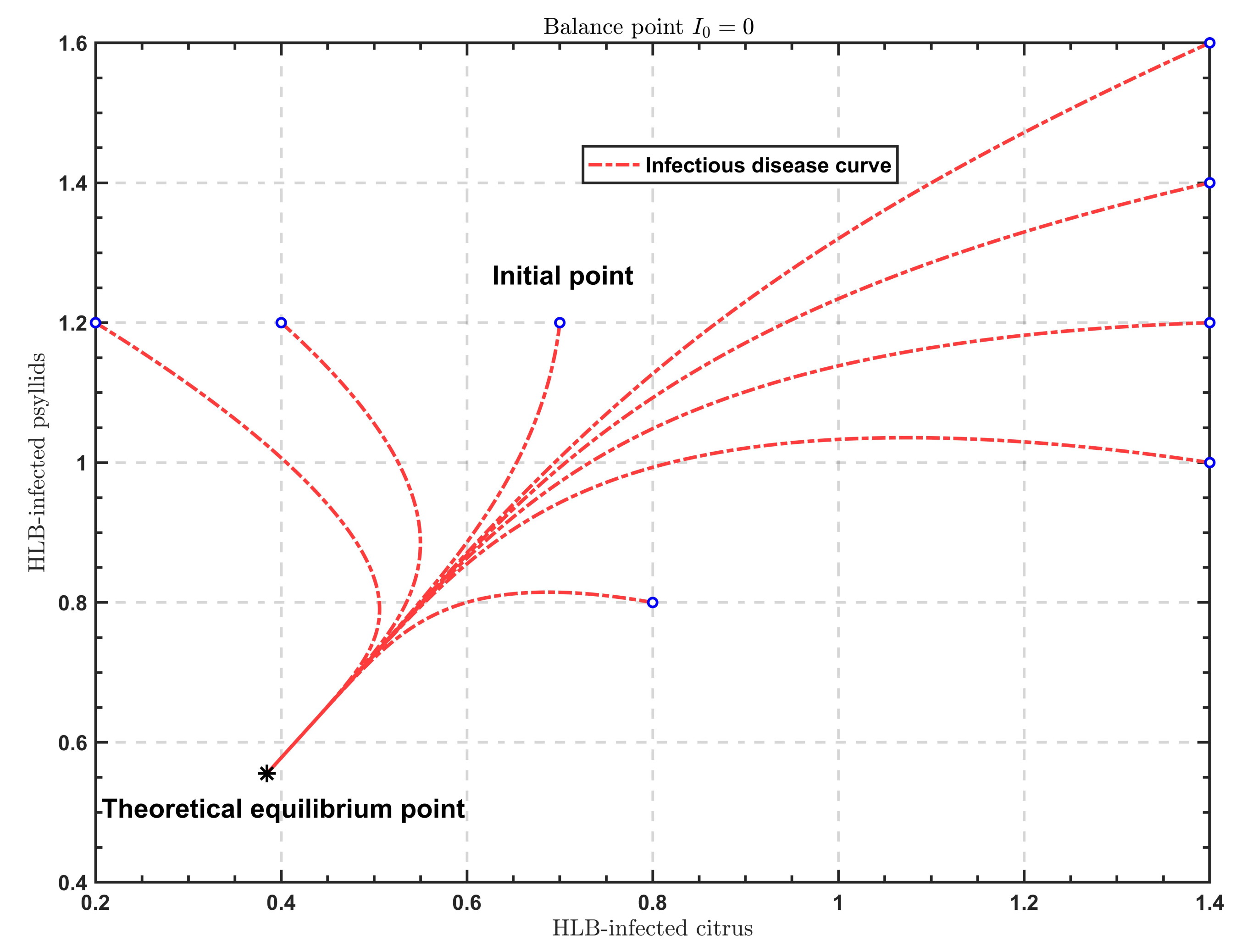
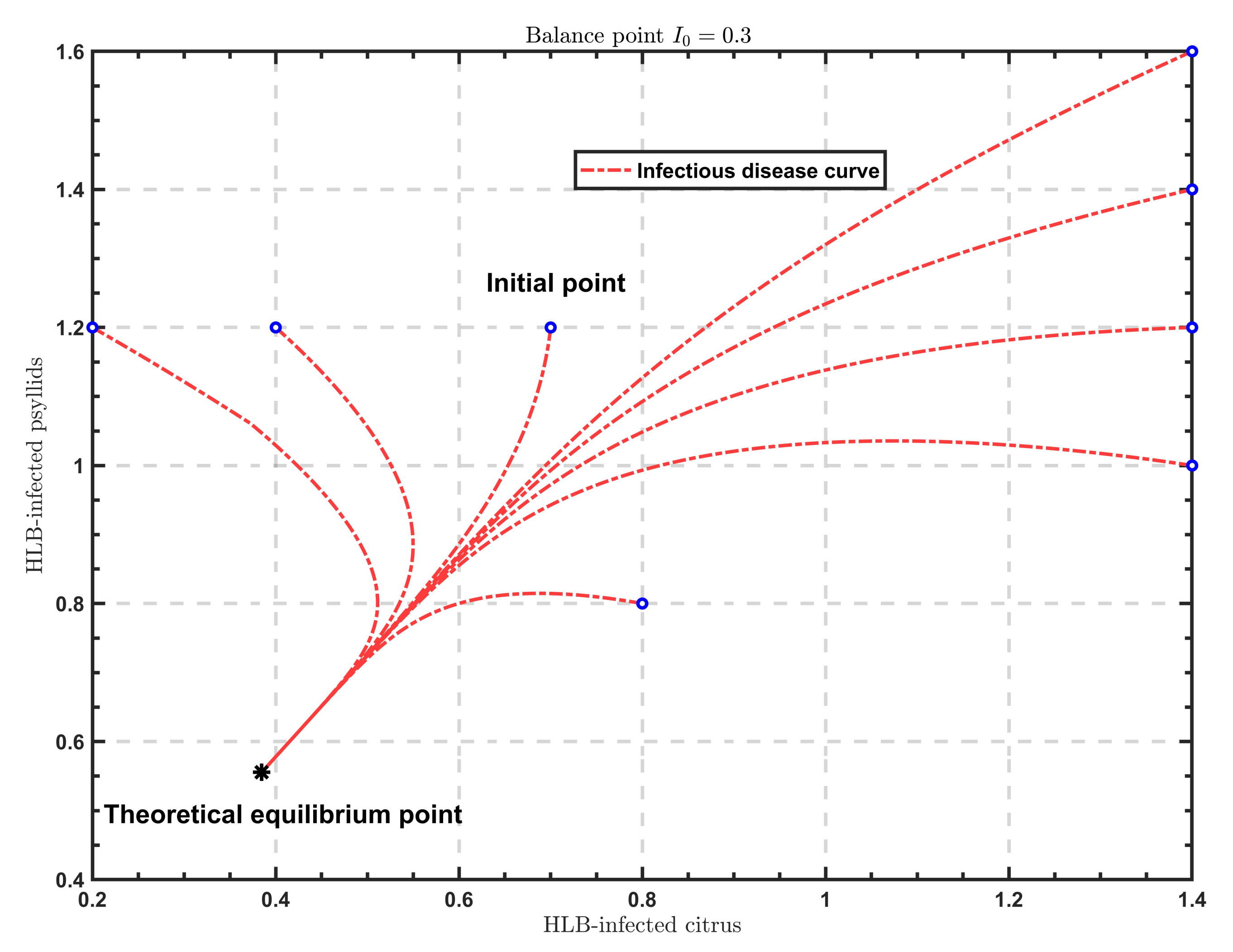
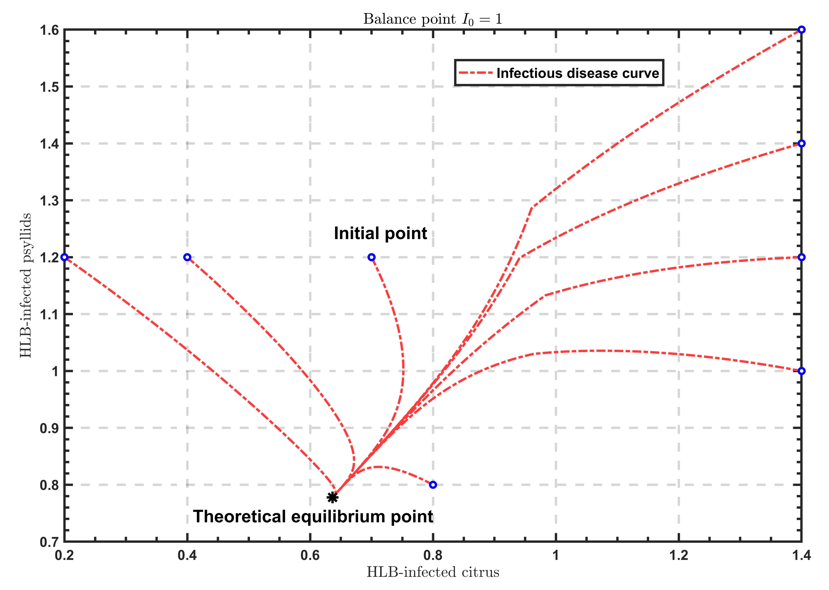
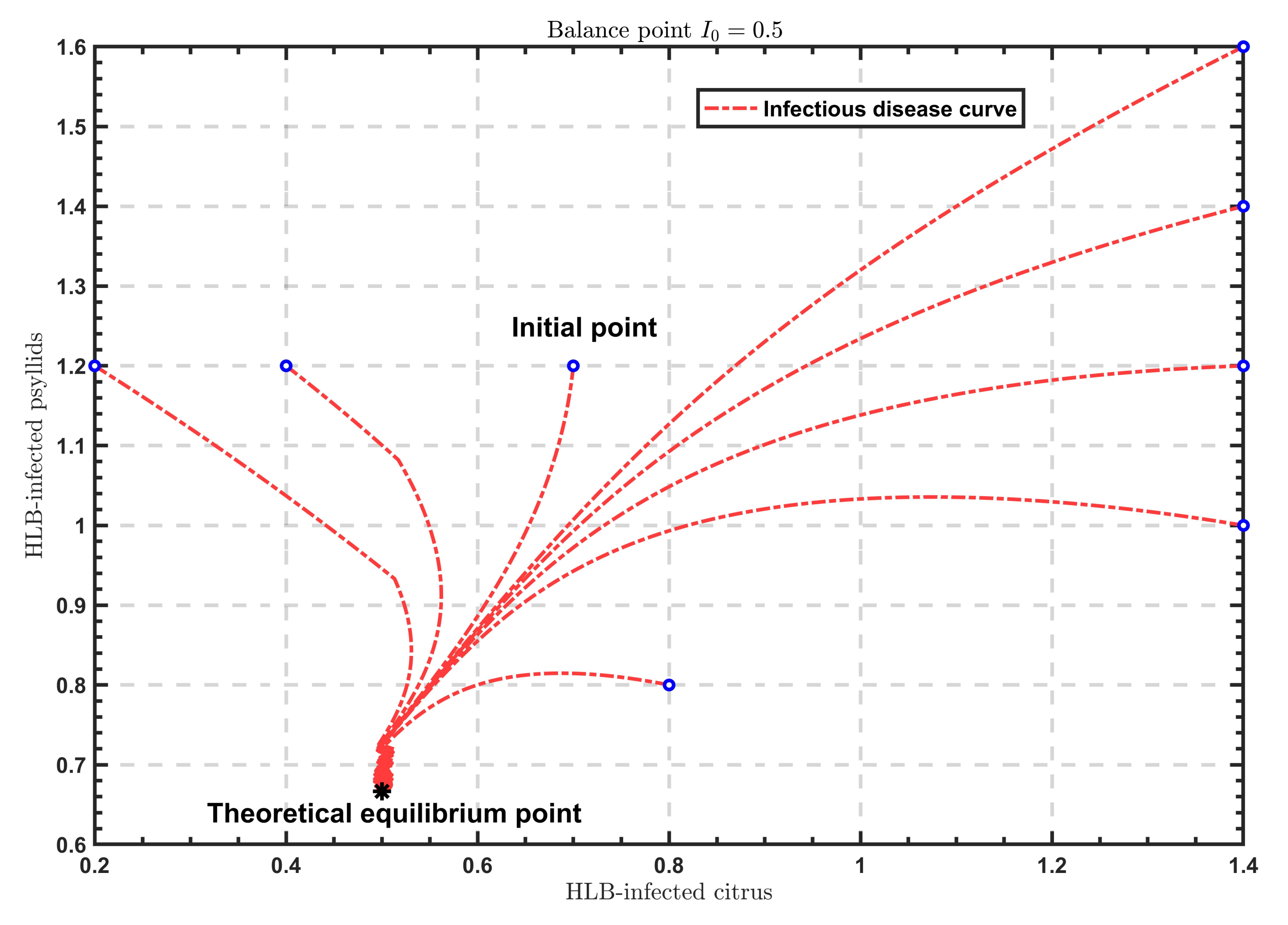
As shown in Figure 2, Figure 3 and Figure 4, when $I_0=1>0.64$, the solutions all tend to the endemic equilibrium $E_{*}^{-}=\left(0.64,0.78\right)$; in the case of $I_0=0.3<0.38$, the solutions all stabilize at the endemic equilibrium $E_{*}^{+}=\left(0.38,0.55\right)$; when $I_0=0.5\in [0.38,0.64]$, the solutions all approximate to the endemic equilibrium $E_{*}=\left(0.5,0.67\right)$. Above all, when $I_0$ varies, the model will show different endemic equilibria; however, regardless of the value of $I_0$, the solutions $\left(I_h\left(t\right),I_v\left(t\right)\right)$ under different initial values eventually approximate to the endemic equilibrium. Therefore, the endemic equilibrium exhibits globally asymptotic stability.

5. Conclusions

According to the characteristics of HLB disease and the characteristics of control measures for removing infected trees, reasonable assumptions are proposed. Moreover, by selecting proper parameters and reasonable functions, the influence of the control strategy of discontinuously removing infected trees on HLB disease is described. Furthermore, a corresponding mathematical model was established to explore the dynamic properties of the system. Through numerical simulation, the existence and global stability of the resulting equilibria were validated. Additionally, it was found that different values of $I_0$ do not change the dynamic properties of HLB disease. However, the lower the value of $I_0$ is, the fewer HLB-infected citrus trees there are. When $R_1$ is less than or equal to 1, the model only has a disease-free equilibrium point that is globally asymptotically stable. This means that fruit growers can artificially increase the removal rate of diseased trees so that $R_1$ is less than or equal to 1. Huanglongbing disease will gradually disappear at this time. Of course, the cost of control will be more. When $R_1$ is greater than 1, the model has a globally asymptotically stable endemic equilibrium point, which means that Huanglongbing disease will continue to develop. The value of $I_0$ will not change the dynamic properties of Huanglongbing disease; however, the smaller the value of $I_0$ is, the less citrus will be infected. A small value of $I_0$ means that the removal of diseased trees is increased when there are few infected citrus. At this time, the cost of removing diseased trees will also increase, and after the final stabilization, the less diseased citrus will be, and the corresponding citrus sales revenue will be increased. When $R_1$ is less than or equal to 1, the model only has a disease-free equilibrium point that is globally asymptotically stable. This means that fruit growers can artificially increase the removal rate of diseased trees so that $R_1$ is less than or equal to 1. Huanglongbing disease will gradually disappear at this time. Of course, the cost of control will be increased. When $R_1$ is greater than 1, the model has a globally asymptotically stable endemic equilibrium point, which means that Huanglongbing disease will continue to develop. The value of $I_0$ will not change the dynamic properties of Huanglongbing disease, but the smaller the value of $I_0$, the less citrus will be infected. A small value of $I_0$ means that the removal of diseased trees is increased when there are few infected citrus. At this time, the cost of removing diseased trees will also increase, and after the final stabilization, the less diseased citrus there will be, and the corresponding citrus sales revenue will be increased. This research provides a theoretical basis for fruit growers trying to control HLB disease and reducing expenditure thereon.