
Study of Atmospheric Turbidity in a Northern Tropical Region Using Models and Measurements of Global Solar Radiation

 , ,
, ,  , ,
, ,
Abstract
1. Introduction
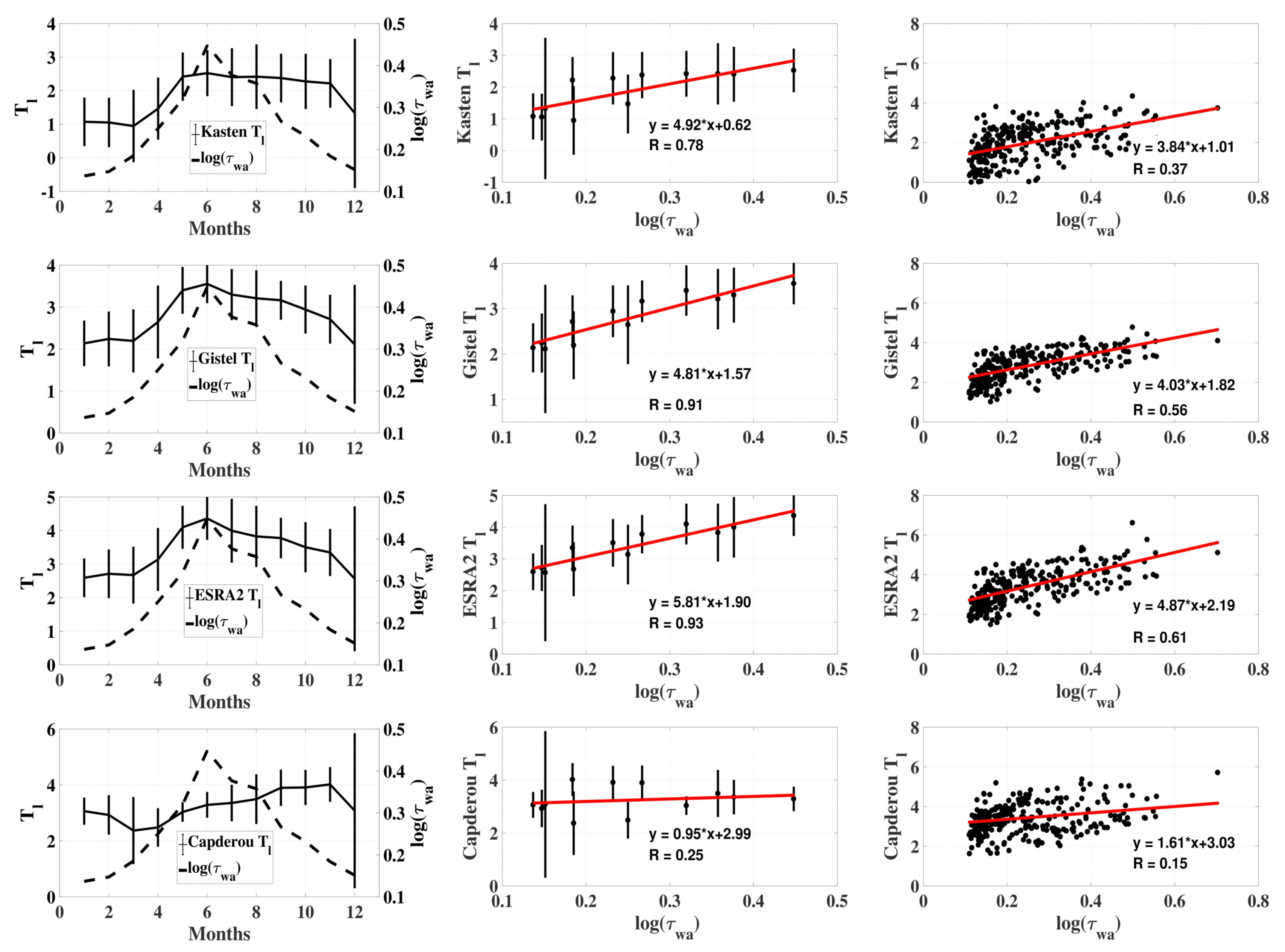
2. Turbidity Models
2.1. The Gistel Model
2.2. The Kasten Model
2.3. The ESRA 1 Model
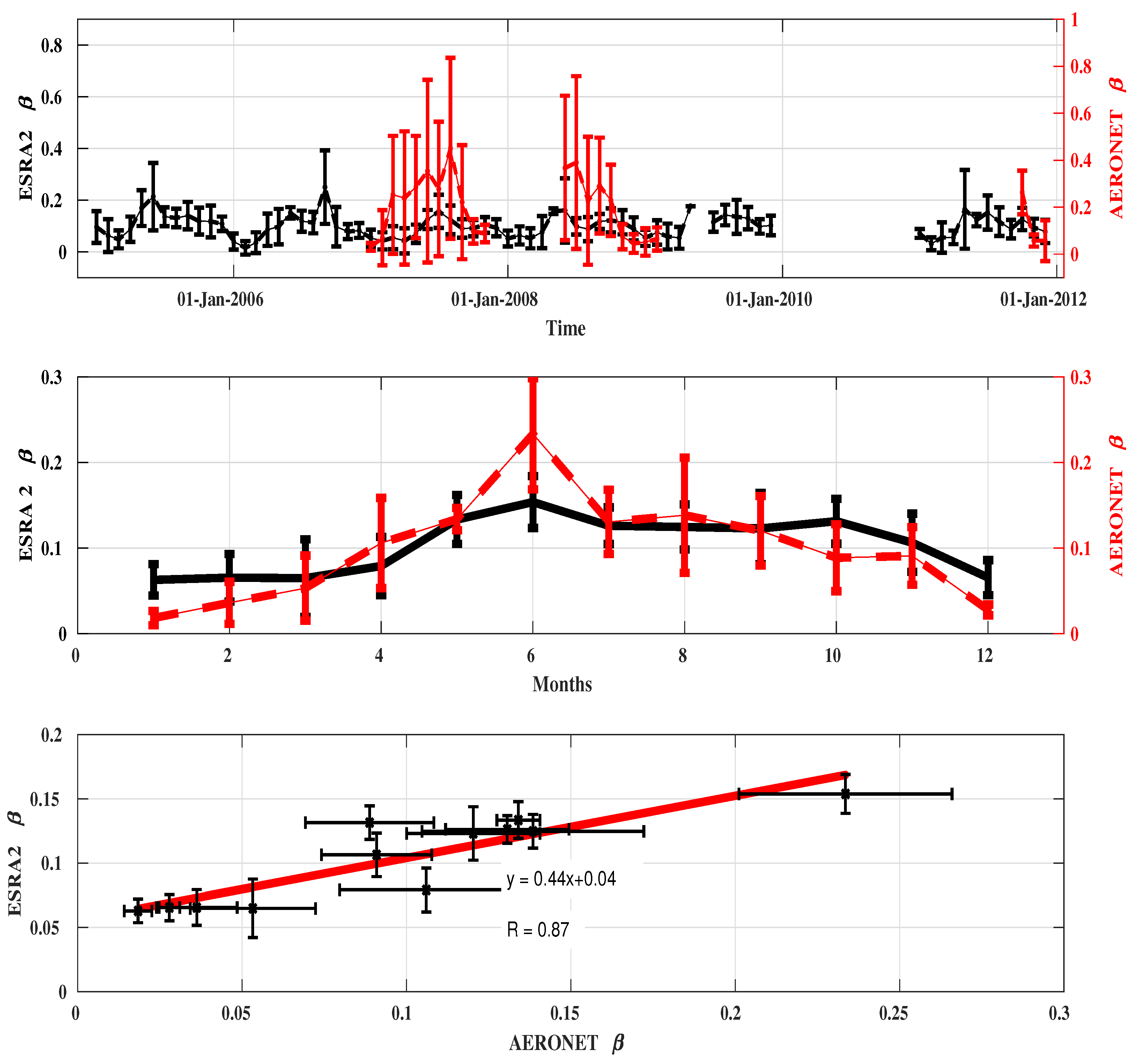
2.4. The ESRA 2 Model
2.5. The Capderou Model
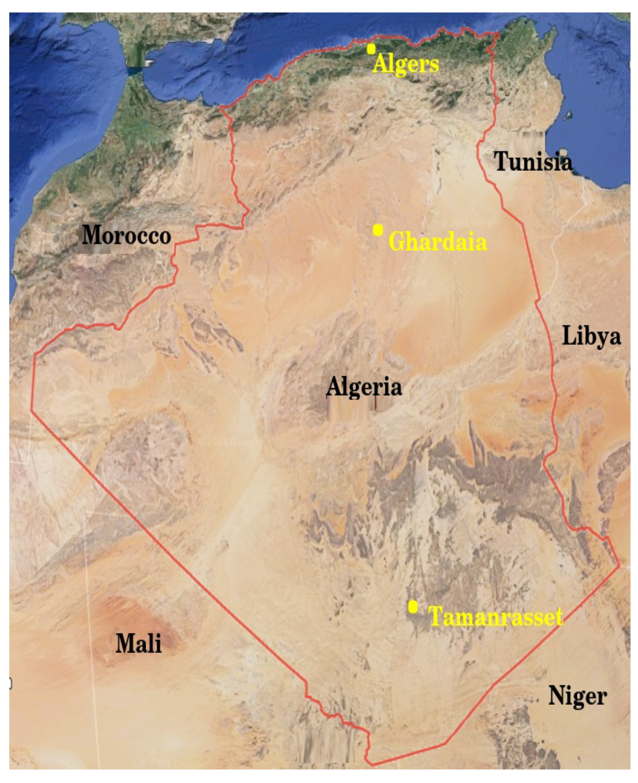
3. Used Data and Site Location
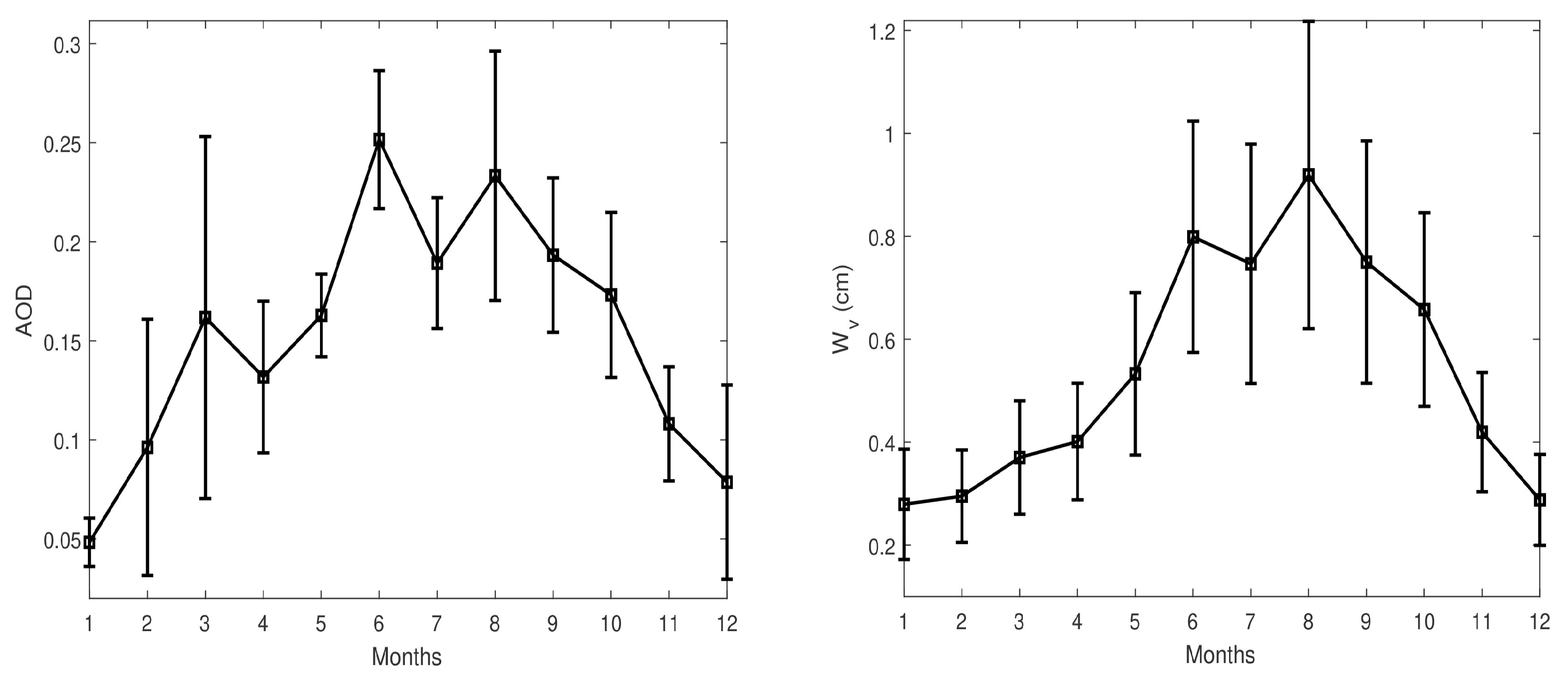
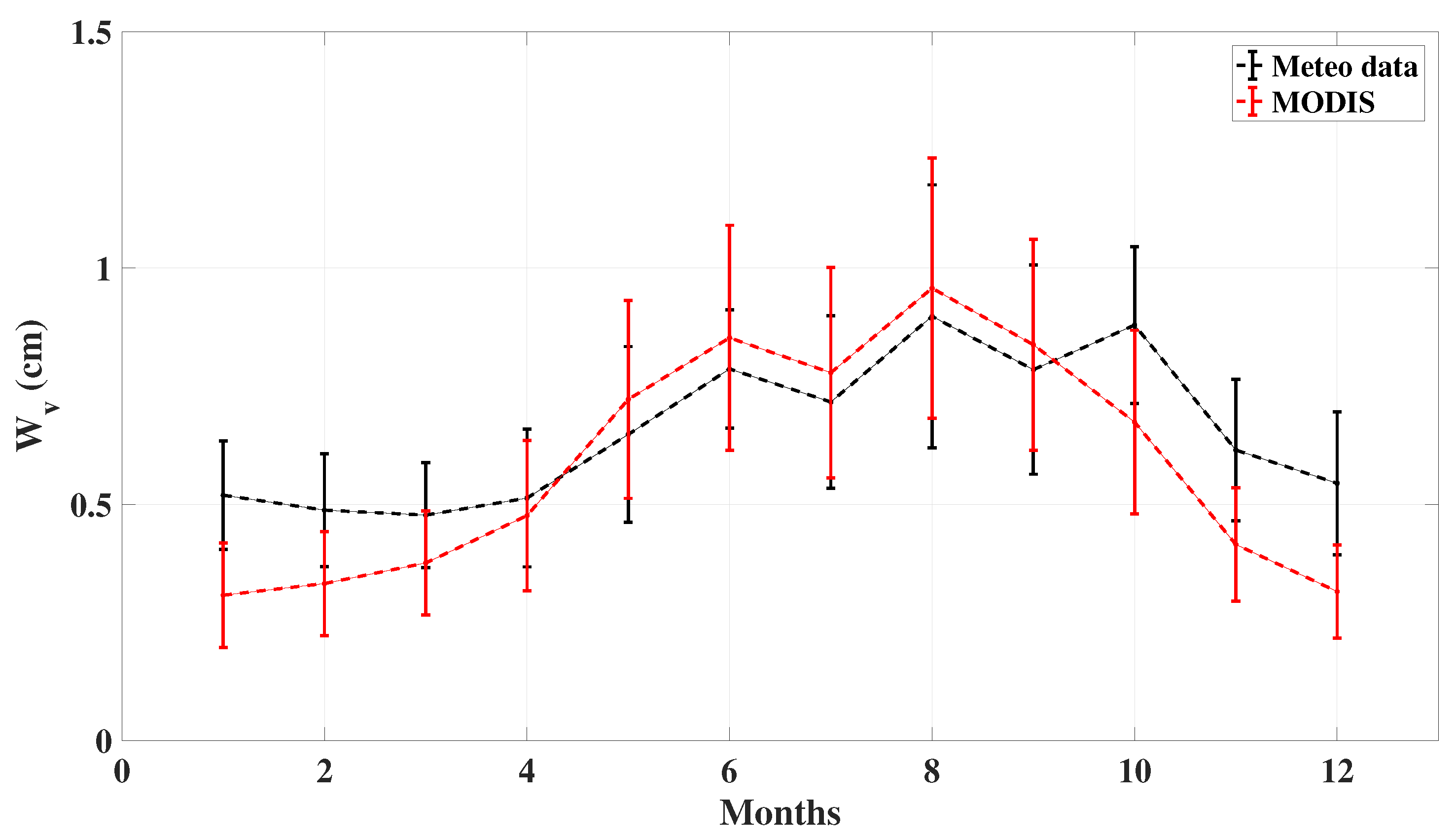
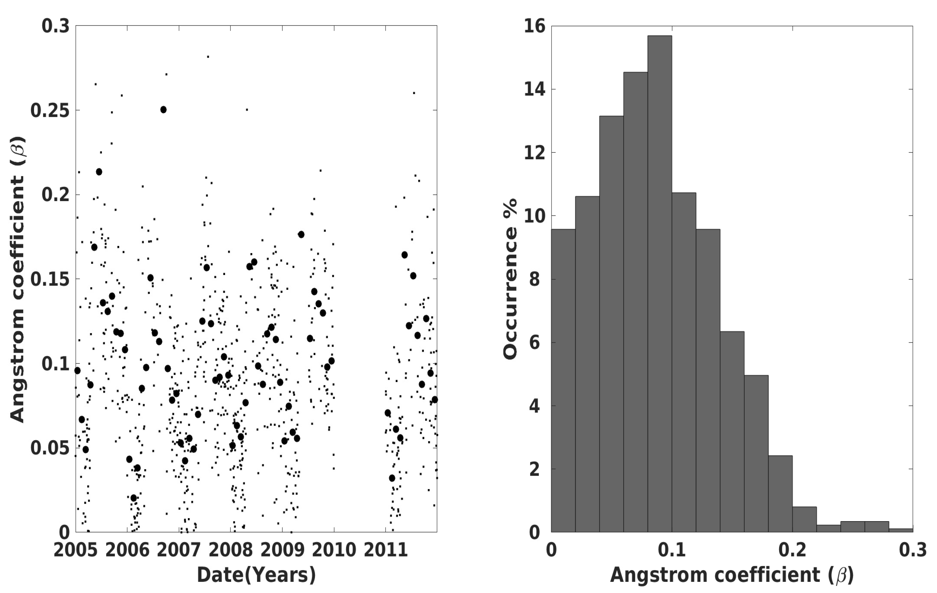
3.1. Aeronet and Modis Data
3.2. Ground-Based Solar Radiation Data
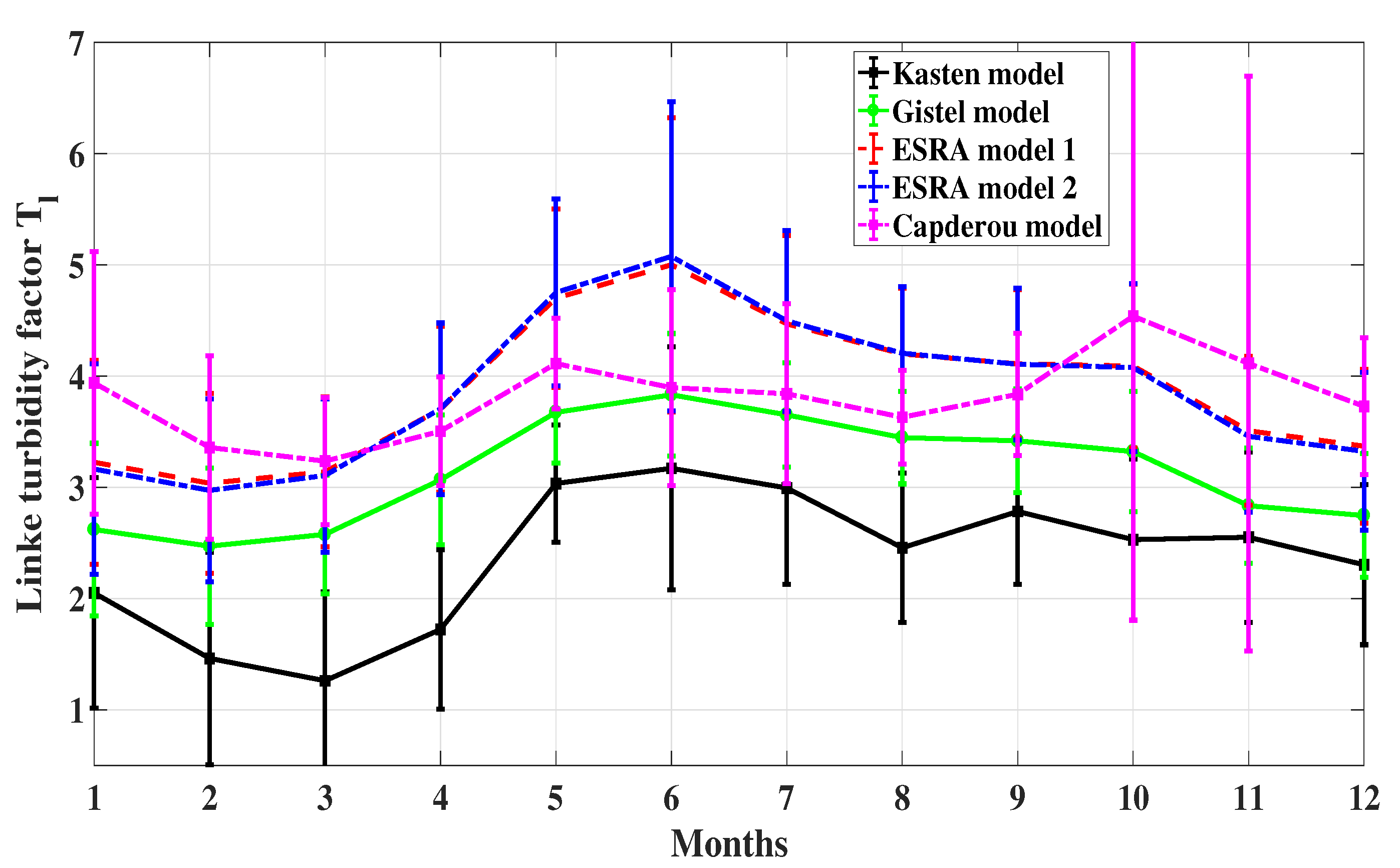
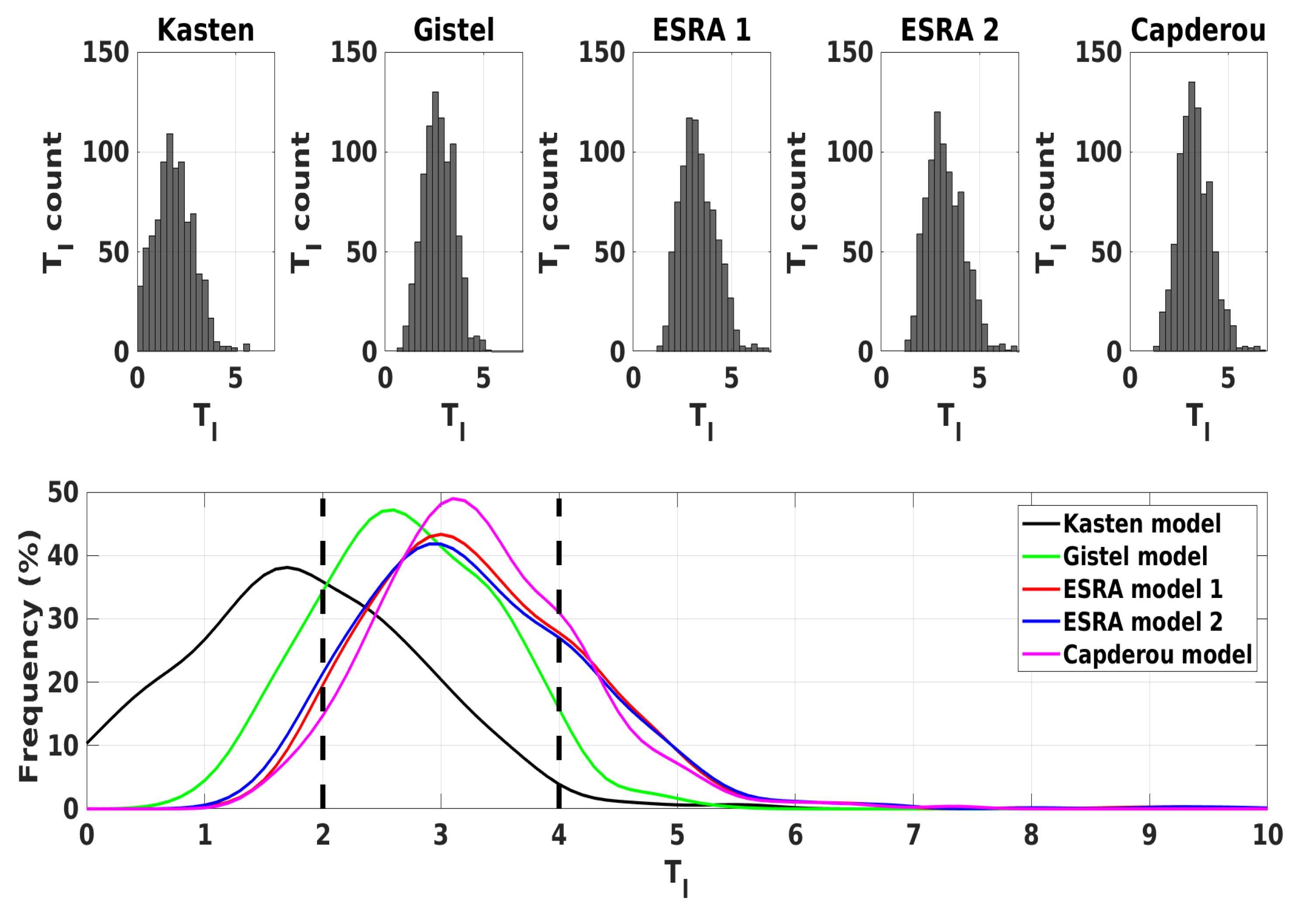
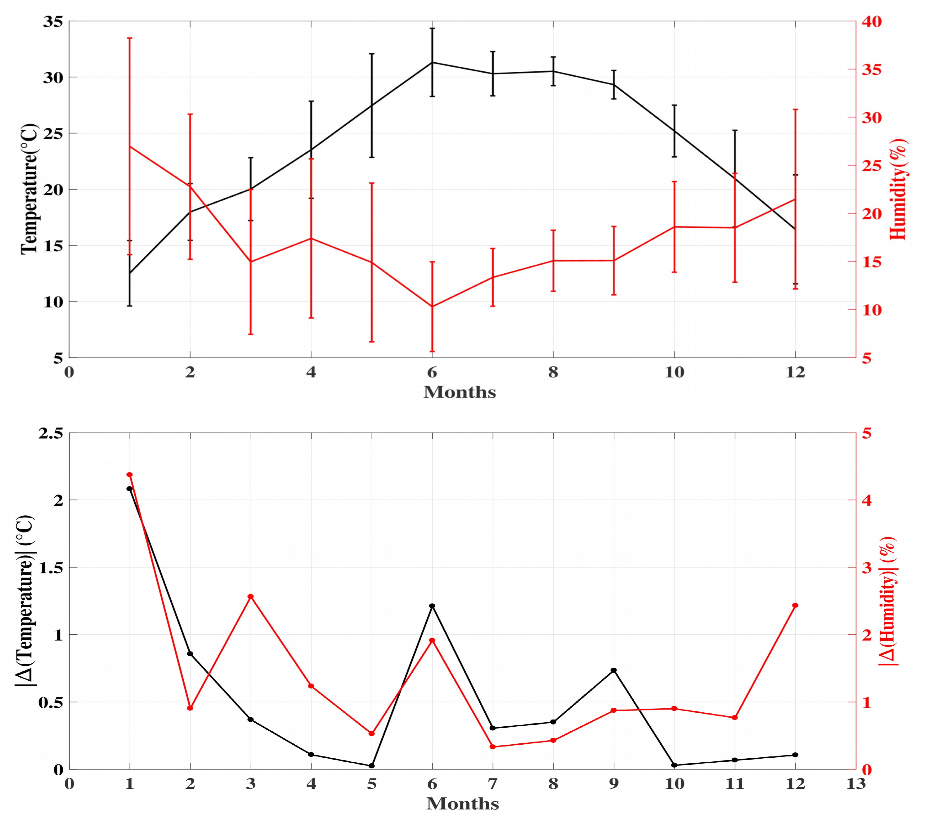
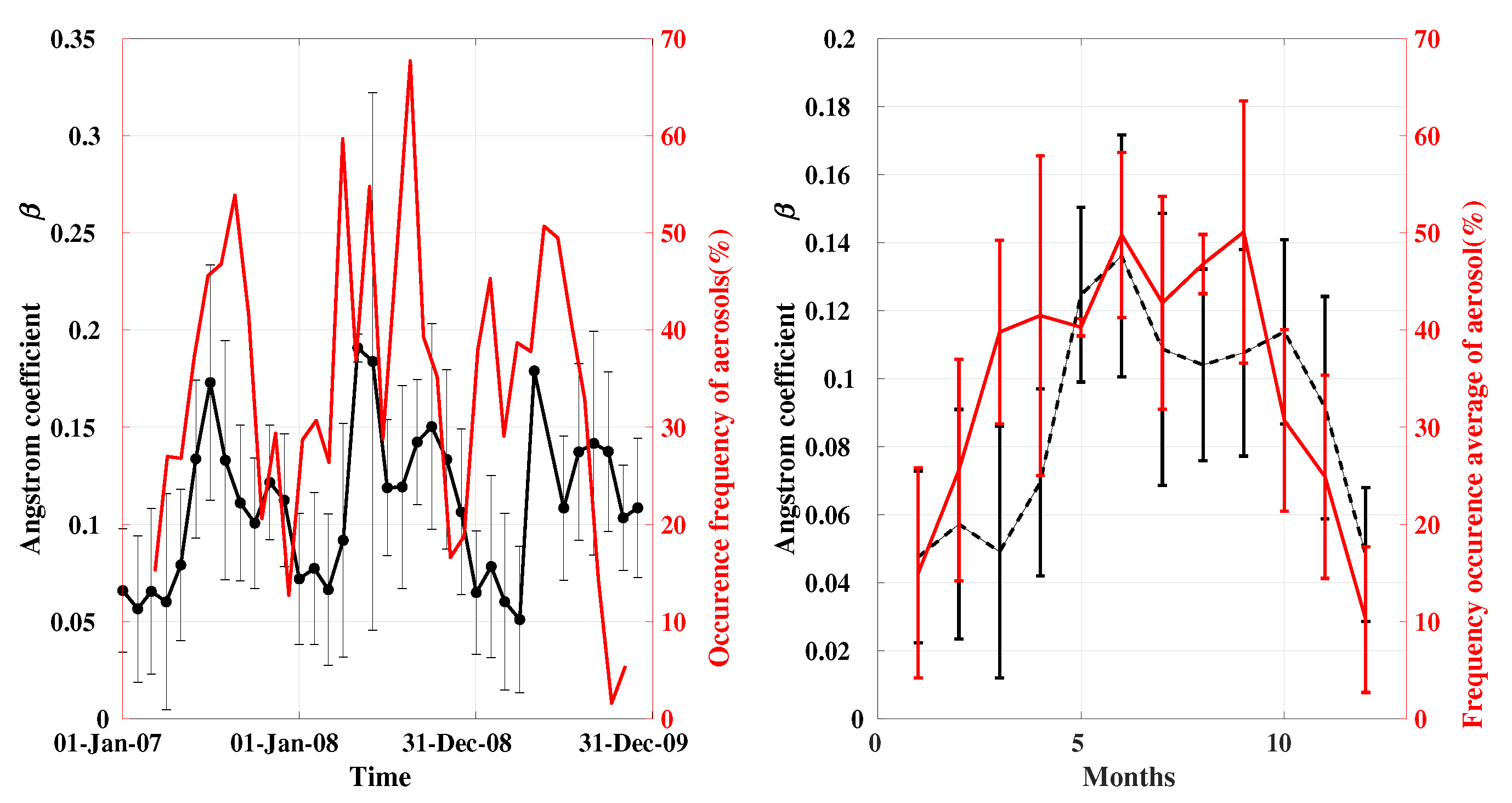
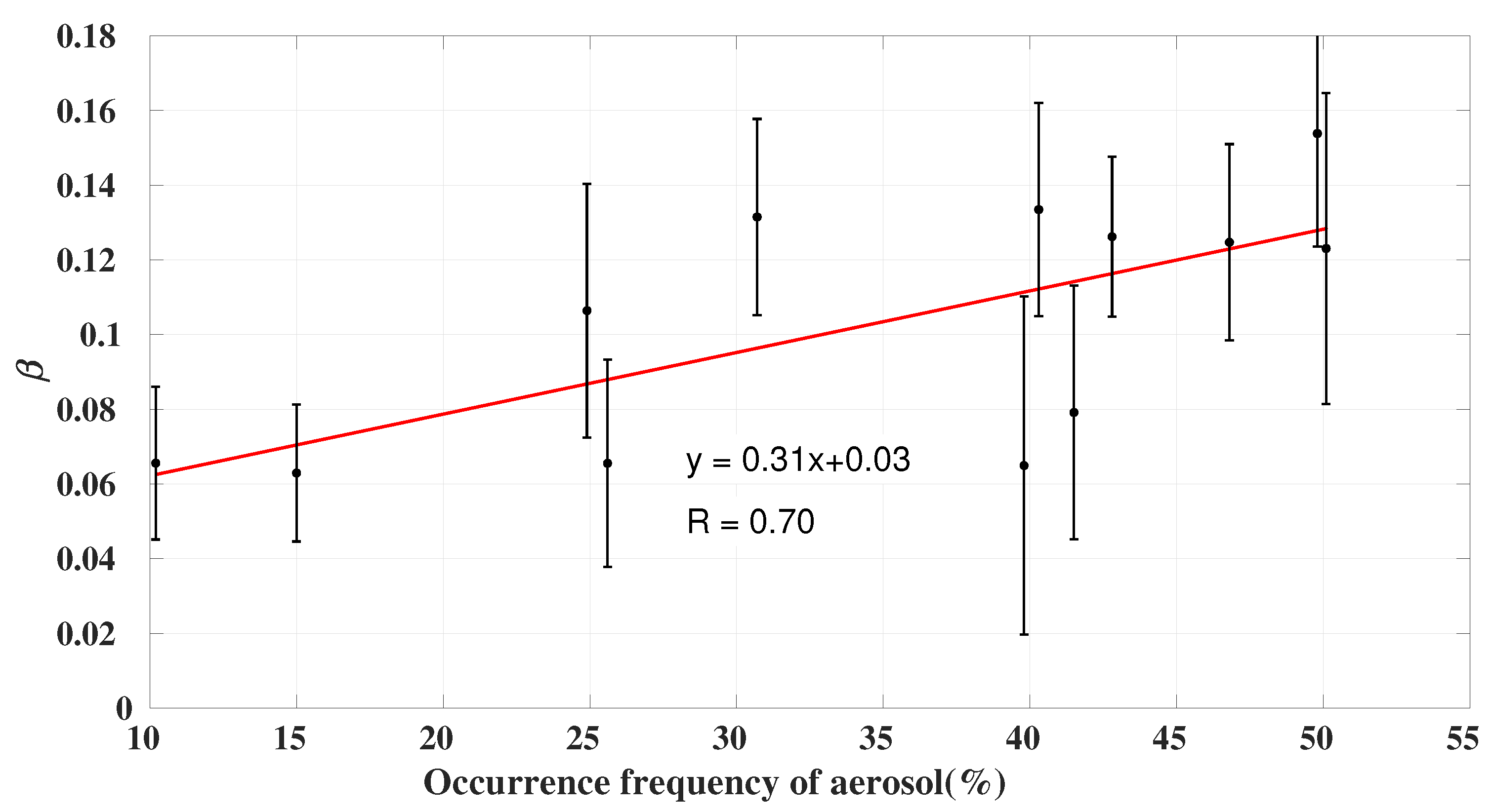
4. Results and Discussion
- is obtained using the formula given in Iqbal [38] of the transmittance following absorption by water vapor:where is the pressure-corrected relative optical path length for water vapor:where is the total column-integrated water vapor abundance and m the optical air mass.
- is calculated through the transmittance formula given in Louche [39] of aerosol scattering and is dependent on the optical air mass m, the Angström coefficient and the Angström exponent :

5. Conclusions
Author Contributions
Funding
Data Availability Statement
Acknowledgments
Conflicts of Interest
References
- Trabelsi, A.; Masmoudi, M. An investigation of atmospheric turbidity over Kerkennah Island in Tunisia. Atmos. Res. 2011, 22, 101. [Google Scholar] [CrossRef]
- Malik, A. A modified method of estimating Angström’s turbidity coefficient of solar radiation models. Renew. Energy 2000, 21, 537. [Google Scholar] [CrossRef]
- Kaskaoutis, D.; Kambezidis, H.; Adamopoulos, A.; Kassomenos, P. Comparison between experimental data and modeling estimates of aerosol optical depth over Athens, Greece. J. Atmos. Sol. Terr. Phys. 2006, 68, 1167–1178. [Google Scholar] [CrossRef]
- Kosmopoulos, P.; Kazadzis, S.; El-Askary, H.; Taylor, M.; Gkikas, A.; Proestakis, E.; Kontoes, C.; El-Khayat, M. Earth-Observation-Based Estimation and Forecasting of Particulate Matter Impact on Solar Energy in Egypt. Remote Sens. 2018, 10, 1870. [Google Scholar] [CrossRef]
- Kambezidis, H.; Adamopoulos, A.; Zevgolis, D. Spectral aerosol transmittance in the ultraviolet and visible spectrum in Athens, Greece. Pure Appl. Geophys. 2005, 162, 625–647. [Google Scholar] [CrossRef]
- Kaskaoutis, D.; Kambezidis, H.; Jacovides, C.; Steven, M. Modification of solar radiation components under different atmospheric conditions in the greater Athens area, Greece. J. Atmos. Sol. Terr. Phys. 2006, 68, 1043–1052. [Google Scholar] [CrossRef]
- Kaskaoutis, D.; Kambezidis, H. Investigationon the wavelength dependence of the aerosol optical depth in the Athens area. Q. J. R. Meteorol. Soc. 2006, 132, 2217–2235. [Google Scholar] [CrossRef]
- Kaskaoutis, D.; Kambezidis, H. The diffuse-to-globa land diffuse-to-direct-beam spectral irradiance ratios as turbidity indexes in an urban environment. J. Atmos. Sol. Terr. Phys. 2009, 71, 246–256. [Google Scholar] [CrossRef]
- Gueymard, C. Clear-sky irradiance predictions for solar resource mapping and large-scale applications: Improved validation methodology and detailed performance analysis of 18 broadband radiative models. Sol. Energy 2012, 86, 2145–2169. [Google Scholar] [CrossRef]
- Antonanzas-Torres, F.; Urraca, R.; Polo, J.; Perpiñán-Lamigueiro, O.; Escobar, R. Clear sky solar irradiance models: A review of seventy models. Renew. Sustain. Energy Rev. 2019, 107, 374–387. [Google Scholar] [CrossRef]
- Badescu, V.; Gueymard, C.; Cheval, S.; Oprea, C.; Baciu, M.; Dumitrescud, A.; Iacobescu, F.; Milos, I.; Rada, C. Computing global and diffuse solar hourly irradiation on clear sky: Review and testing of 54 models. Renew. Sustain. Energy Rev. 2012, 16, 1636–1656. [Google Scholar] [CrossRef]
- Kambezidis, H.; Psiloglou, B.; Karagiannis, D.; Kaskaoutis, U.D.D. Recent improvements of the Meteorological Radiation Model for solar irradiance estimates under all-sky conditions. Renew Energy 2016, 93, 142–158. [Google Scholar] [CrossRef]
- Kambezidis, H.; Psiloglou, B.; Karagiannis, D.; Dumka, U.; Kaskaoutis, D. Meteorological Radiation Model (MRM v6.1): Improvements in diffuse radiation estimates and a new approach for implementation of cloud products. Renew. Sustain. Energy Rev. 2017, 74, 616–637. [Google Scholar] [CrossRef]
- Gueymard, C. SMARTS2, A Simple Model of the Atmospheric Radiative Transfer of Sunshine: Algorithms and Performance Assessment; Rep. FSEC–PF–270–95; Florida Solar Energy Center: Cocoa, FL, USA, 1995. [Google Scholar]
- Linke, F. Transmissions-Koeffizient und Trübungsfaktor. Beitr. Phys. Atmos. 1922, 10, 91–103. [Google Scholar]
- Angström, A. Techniques of determining the turbidity of the atmosphere. Tellus 1961, 13, 214. [Google Scholar] [CrossRef]
- Ineichen, P.; Perez, R. A New Airmass Independent Formulation For The Linke Turbidity Coefficient. Sol. Energy 2002, 73, 151–157. [Google Scholar] [CrossRef]
- Cucumo, M.; Marinelli, V.; Oliveti, G. Data bank Experimental data of the Linke Turbidity factor and estimates of the Ångström turbidity coefficient for two Italian localities. Renew. Energy 1999, 17, 397–410. [Google Scholar] [CrossRef]
- Djafer, D.; Irbah, A. Estimation of atmospheric turbidity over Ghardaïa city. Atmos. Res. 2013, 128, 76–84. [Google Scholar] [CrossRef]
- Marif, Y.; Bechki, D.; Zerrouki, M.; Belhadj, M.; Bouguettaia, H.; Benmoussa, H. Estimation of atmospheric turbidity over Adrar city in Algeria. J. King Saud Univ. Sci. 2019, 31, 143–149. [Google Scholar] [CrossRef]
- Chabane, F.; Moummi, N.; Brima, A. A New Approach to Estimate the Distribution of Solar Radiation Using Linke Turbidity Factor and Tilt Angle. Trans. Mech. Eng. 2021, 45, 523–534. [Google Scholar] [CrossRef]
- Saad, M.; Trabelsi, A.; Masmoudi, M.; Alfaro, S.C. Spatial and temporal variability of the atmospheric turbidity in Tunisia. J. Atmos. Sol. Terr. Phys. 2016, 149, 93–99. [Google Scholar] [CrossRef]
- Kambezidis, H.D.; Psiloglou, B.E. Climatology of the Linke and Unsworth—Monteith Turbidity Parameters for Greece: Introduction to the Notion of a Typical Atmospheric Turbidity Year. Appl. Sci. 2020, 10, 4043. [Google Scholar] [CrossRef]
- Zakey, A.S.; Abdelwahab, M.M.; Makar, P.A. Atmospheric turbidity over Egypt. Environment 2004, 38, 1579–1591. [Google Scholar] [CrossRef]
- Behar, O.; Sbarbaro, D.; Marzo, A.; Moran, L. A simplified methodology to estimate solar irradiance and atmospheric turbidity from ambient temperature and relative humidity. Renew. Sustain. Energy Rev. 2019, 116, 109310. [Google Scholar] [CrossRef]
- Flores, J.L.; Karam, H.A.; Marques Filho, E.P.; Pereira Filho, A.J. Estimation of atmospheric turbidity and surface radiative parameters using broadband clear sky solar irradiance models in Rio de Janeiro-Brasil. Theor. Appl. Climatol. 2016, 123, 593–617. [Google Scholar] [CrossRef]
- Meziani, F.; Boulifa, M.; Ameur, Z. Determination of the global solar irradiation by MSG-SEVIRI images processing in Algeria. Energy Procedia 2013, 36, 525–534. [Google Scholar] [CrossRef]
- Mefti, A.; Adane, A.; Bouroubi, M. A Satellite approach based on cloud cover classification: Estimation of hourly global solar radiation from meteosat images. Energy Convers. Manag. 2008, 49, 652–659. [Google Scholar] [CrossRef]
- Davies, J.; Mckay, D. Evaluation of Selected Models for Estimating Solar Radiation on Horizontal Surfaces. Sol. Energy 1989, 43, 153–168. [Google Scholar] [CrossRef]
- Rigollier, C.; Bauer, O.; Wald, L. On the clear sky model of the ESRA—European Solar Radiation Atlas- with respect to the heliosat method. Sol. Energy 2000, 68, 22–48. [Google Scholar] [CrossRef]
- Capdrou, M. Atlas Solaire de l’Algérie, Modèles Théoriques et Expérimentaux; Office des Publications Universitaires: Algiers, Algeria, 1987; Volume 1. [Google Scholar]
- Marif, Y.; Chiba, Y.; Belhadj, M.; Zerrouki, M.; Benhammou, M. Clear Sky Irradiation Assessment Using A Modified Algerian Solar Atlas Model in Adrar City. Energy Rep. 2018, 4, 84–90. [Google Scholar] [CrossRef]
- Yaiche, M.; Bekkouche, A.B.S.; Malek, A.; Benouaz, T. Revised Solar Maps of Algeria Based on Sunshine Duration. Energy Convers. Manag. 2014, 82, 114–123. [Google Scholar] [CrossRef]
- Brichambaut, P.; Vauge, C. Le Gisement Solaire: évaluation de la ressource énergétique; Lavoisier: Paris, France, 1982. [Google Scholar]
- Zaiani, M.; Djafer, D. Atmospheric Turbidity Study Using Ground and Orbit Data. Int. J. Latest Res. Sci. Technol. 2014, 3, 12–18. [Google Scholar]
- Zaiani, M.; Djafer, D.; Chouireb, F. New Approach to Establish a Clear Sky Global Solar Irradiance Model. Int. J. Renew. Energy Res. 2017, 7, 1454–1462. [Google Scholar]
- Zaiani, M.; Djafer, D.; Chouireb, F.; Irbah, A.; Hamidia, M. New Method for Clear Day Selection Based on Normalized Least Mean Square Algorithm. Theor. Appl. Climatol. 2019, 1–8. [Google Scholar] [CrossRef]
- Iqbal, M. An Introduction to Solar Radiation; Academic Press: Toronto, ON, Canada, 1983. [Google Scholar]
- Louche, A.; Maurel, M.; Simonnot, G.; Peri, G.; Iqbal, M. Determination of Ångström’s turbidity coefficient from direct total solar irradiance measurements. Sol. Energy 1987, 38, 89–96. [Google Scholar] [CrossRef]
- Lopez, G.; Batlles, F. Estimate of the atmospheric turbidity from three broad-band solar radiation algorithms, a comparative study. Ann. Geophys 2004, 22, 2657–2668. [Google Scholar] [CrossRef]
- Djelloul, D.; Abdanour, I.; Philippe, K.; Mohamed, Z.; Mustapha, M. Investigation of Atmospheric Turbidity at Ghardaïa (Algeria) Using Both Ground Solar Irradiance Measurements and Space Data. Atmos. Clim. Sci. 2019, 9, 114–134. [Google Scholar] [CrossRef][Green Version]
- Cuesta, J.; Edouart, D.; Mimouni, M.; Flamant, P.; Loth, C.; Gibert, F.; Marnas, F.; Bouklila, A.; Kharef, M.; Ouchène, B.; et al. Multiplatform observations of the seasonal evolution of the Saharan atmospheric boundary layer in Tamanrasset, Algeria, in the framework of the African Monsoon Multidisciplinary Analysis field campaign conducted in 2006. J. Geophys. Res. 2008, 113. [Google Scholar] [CrossRef]
- Delanoe, J.; Hogan, R. Combined CloudSat-CALIPSO-MODIS retrievals of the properties of ice clouds. J. Geophys. Res. 2010, 115. [Google Scholar] [CrossRef]
- Ceccaldi, M.; Delanoë, J.; Hogan, R.; Pounder, N.; Protat, A.; Pelon, J. From CloudSat-CALIPSO to EarthCare: Evolution of the DARDAR cloud classification and its comparison to airborne radar-lidar observations. J. Geophys. Res. 2013, 118, 7962–7981. [Google Scholar] [CrossRef]
- Cazenave, Q.; Ceccaldi, M.; Delanoë, J.; Pelon, J.; Groß, S.; Heymsfield, A. Evolution of DARDAR-CLOUD ice cloud retrievals: New parameters and impacts on the retrieved microphysical properties. Atmos. Meas. Tech. 2019, 12, 2819–2835. [Google Scholar] [CrossRef]
- Stephens, G.; Vane, D.; Boain, R.; Mace, G.; Sassen, K.; Wang, Z.; Illingworth, A.; O’Connor, E.; Rossow, W.; Durden, S.; et al. The CloudSat Mission and the A-Train. Bull. Am. Meteorol. Soc. 2002, 83, 1771–1790. [Google Scholar] [CrossRef]
- Winker, D.; Pelon, J.; Coakley, J.; Ackerman, S.; Charlson, R.; Colarco, P.; Flamant, P.; Fu, Q.; Hoff, R.; Kit-taka, C.; et al. The CALIPSO Mission: A global 3D view of aerosols and clouds. Bull. Am. Meteorol. Soc. 2010, 91, 1211–1229. [Google Scholar] [CrossRef]


| Errors/Models | Kasten | Gistel | ESRA1 | ESRA2 | Capderou |
|---|---|---|---|---|---|
| (W/m2) | 29.52 | 18.34 | 14.84 | 13.44 | 16.13 |
| (%) | 10.34 | 10.95 | 12.50 | 6.44 | 15.22 |
| (W/m2) | 1.03 | 4.26 | 2.58 | −0.64 | 3.82 |
| R | 0.9981 | 0.9991 | 0.9994 | 0.9995 | 0.9993 |
| Months | 2005 | 2006 | 2007 | 2008 | 2009 | 2011 |
|---|---|---|---|---|---|---|
| January | 0.10 ± 0.06 | 0.09 ± 0.06 | 0.09 ± 0.06 | 0.07 ± 0.06 | 0.09 ± 0.06 | 0.09 ± 0.06 |
| February | 0.06 ± 0.04 | 0.08 ± 0.07 | 0.05 ± 0.04 | 0.06 ± 0.03 | 0.07 ± 0.06 | 0.06 ± 0.06 |
| March | 0.05 ± 0.03 | 0.05 ± 0.03 | 0.06 ± 0.04 | 0.14 ± 0.08 | 0.05 ± 0.04 | 0.06 ± 0.03 |
| April | 0.09 ± 0.05 | 0.09 ± 0.05 | 0.16 ± 0.05 | 0.13 ± 0.04 | 0.06 ± 0.04 | 0.08 ± 0.05 |
| May | 0.17 ± 0.07 | 0.17 ± 0.06 | 0.18 ± 0.09 | 0.15 ± 0.04 | 0.12 ± 0.01 | 0.16 ± 0.06 |
| June | 0.21 ± 0.13 | 0.21 ± 0.12 | 0.13 ± 0.04 | 0.12 ± 0.04 | - | 0.23 ± 0.10 |
| July | 0.14 ± 0.04 | 0.14 ± 0.03 | 0.15 ± 0.05 | 0.14 ± 0.05 | 0.17 ± 0.09 | 0.14 ± 0.03 |
| August | 0.13 ± 0.04 | 0.13 ± 0.04 | 0.12 ± 0.04 | 0.12 ± 0.05 | 0.15 ± 0.04 | 0.11 ± 0.03 |
| September | 0.14 ± 0.05 | 0.13 ± 0.04 | 0.11 ± 0.06 | 0.11 ± 0.06 | 0.12 ± 0.03 | 0.14 ± 0.04 |
| October | 0.12 ± 0.05 | 0.14 ± 0.04 | 0.09 ± 0.04 | 0.09 ± 0.04 | 0.14 ± 0.04 | 0.16 ± 0.08 |
| November | 0.12 ± 0.06 | 0.13 ± 0.05 | 0.02 ± 0.03 | 0.02 ± 0.02 | 0.14 ± 0.05 | 0.11 ± 0.04 |
| December | 0.11 ± 0.03 | 0.11 ± 0.05 | 0.03 ± 0.05 | 0.03 ± 0.03 | 0.12 ± 0.06 | 0.11 ± 0.05 |
Publisher’s Note: MDPI stays neutral with regard to jurisdictional claims in published maps and institutional affiliations. |
© 2021 by the authors. Licensee MDPI, Basel, Switzerland. This article is an open access article distributed under the terms and conditions of the Creative Commons Attribution (CC BY) license (https://creativecommons.org/licenses/by/4.0/).
Share and Cite
Zaiani, M.; Irbah, A.; Djafer, D.; Listowski, C.; Delanoe, J.; Kaskaoutis, D.; Boualit, S.B.; Chouireb, F.; Mimouni, M. Study of Atmospheric Turbidity in a Northern Tropical Region Using Models and Measurements of Global Solar Radiation. Remote Sens. 2021, 13, 2271. https://doi.org/10.3390/rs13122271
Zaiani M, Irbah A, Djafer D, Listowski C, Delanoe J, Kaskaoutis D, Boualit SB, Chouireb F, Mimouni M. Study of Atmospheric Turbidity in a Northern Tropical Region Using Models and Measurements of Global Solar Radiation. Remote Sensing. 2021; 13(12):2271. https://doi.org/10.3390/rs13122271
Chicago/Turabian StyleZaiani, Mohamed, Abdanour Irbah, Djelloul Djafer, Constantino Listowski, Julien Delanoe, Dimitris Kaskaoutis, Sabrina Belaid Boualit, Fatima Chouireb, and Mohamed Mimouni. 2021. "Study of Atmospheric Turbidity in a Northern Tropical Region Using Models and Measurements of Global Solar Radiation" Remote Sensing 13, no. 12: 2271. https://doi.org/10.3390/rs13122271
APA StyleZaiani, M., Irbah, A., Djafer, D., Listowski, C., Delanoe, J., Kaskaoutis, D., Boualit, S. B., Chouireb, F., & Mimouni, M. (2021). Study of Atmospheric Turbidity in a Northern Tropical Region Using Models and Measurements of Global Solar Radiation. Remote Sensing, 13(12), 2271. https://doi.org/10.3390/rs13122271