Soil Organic Matter Prediction Model with Satellite Hyperspectral Image Based on Optimized Denoising Method

Abstract

In order to improve the signal-to-noise ratio of the hyperspectral sensors and exploit the potential of satellite hyperspectral data for predicting soil properties, we took MingShui County as the study area, which the study area is approximately 1481 km², and we selected Gaofen-5 (GF-5) satellite hyperspectral image of the study area to explore an applicable and accurate denoising method that can effectively improve the prediction accuracy of soil organic matter (SOM) content. First, fractional-order derivative (FOD) processing is performed on the original reflectance (OR) to evaluate the optimal FOD. Second, singular value decomposition (SVD), Fourier transform (FT) and discrete wavelet transform (DWT) are used to denoise the OR and optimal FOD reflectance. Third, the spectral indexes of the reflectance under different denoising methods are extracted by optimal band combination algorithm, and the input variables of different denoising methods are selected by the recursive feature elimination (RFE) algorithm. Finally, the SOM content is predicted by a random forest prediction model. The results reveal that 0.6-order reflectance describes more useful details in satellite hyperspectral data. Five spectral indexes extracted from the reflectance under different denoising methods have a strong correlation with the SOM content, which is helpful for realizing high-accuracy SOM predictions. All three denoising methods can reduce the noise in hyperspectral data, and the accuracies of the different denoising methods are ranked DWT > FT > SVD, where 0.6-order-DWT has the highest accuracy (R² = 0.84, RMSE = 3.36 g kg⁻¹, and RPIQ = 1.71). This paper is relatively novel, in that GF-5 satellite hyperspectral data based on different denoising methods are used to predict SOM, and the results provide a highly robust and novel method for mapping the spatial distribution of SOM content at the regional scale.

1. Introduction

The soil organic matter (SOM) is a key variable for evaluating agricultural farmland management, especially regarding edaphic contexts [1], plant physiological dynamics [2] and food security [3]. The fast and low-cost prediction of SOM spatial distributions can provide a timely reference for agricultural farmland management. Visible, near-infrared and shortwave infrared (vis-NIR, 0.4–2.5 μm) spectroscopy can be utilized for the fast, nondestructive, and cost-efficient prediction of the spatial distribution of SOM [4,5,6]. The absorption characteristics of soil spectral reflectance are mainly caused by the overtones and combinations of fundamental vibrations caused by the stretching and bending of N-H, O-H and C-H groups [7]. The significant negative correlation between SOM and soil spectral reflectance is the foundation for prediction of the spatial distribution of SOM [8].

In most previous studies, laboratory-measured hyperspectral data were used to predict SOM content, mainly because this type of data is not easily affected by the soil moisture, soil roughness, atmosphere and environment [9,10,11]. The existence of these interference factors significantly increases the uncertainty in soil property predictions [12,13]. However, compared with laboratory-measured hyperspectral data, satellite hyperspectral data have the advantages of repeated observations and large coverage, which make it possible to predict the spatial distribution of SOM with high accuracy on a large scale [6]. Satellite hyperspectral data contain hundreds of narrow bands and offer more spectral details of the absorption characteristics [14,15,16]. For example, Zhang et al. [17] used Hyperion hyperspectral data of the NASA EO-1 project to predict the SOM, total phosphorus, total nitrogen, total carbon, and clay content of part of the United States and Spain, and Demarchi et al. [18] used Compact High Resolution Imaging Spectrometer (CHRIS) hyperspectral data of the European Space Agency’s Project for On-Board Autonomy to achieve high-accuracy impervious surface mapping. Gaofen-5 (GF-5) hyperspectral data has a full-spectrum range (390–2513 nm), which avoids the problems of low signal-to-noise ratio (SNR) in Hyperion hyperspectral data and narrow band range (415–1050 nm) in CHRIS hyperspectral data. However, in GF-5 hyperspectral data, the noise is mainly produced by the low radiation resolution of the sensor, and the noise has no periodicity [19]. The noise reduces the image quality, affects the accuracy and credibility of information extraction, and sometimes even leads to wrong conclusions [20]. Compared with vegetation, roads, urban areas and other ground objects, for bare soil, the reflectance is low, and the spectrum is more easily affected by noise. The existence of noise limits the potential of hyperspectral data in practical applications. Therefore, reducing the noise of hyperspectral data is essential for obtaining the actual soil spectral reflectance and improving the prediction accuracy [21,22].

Spectral preprocessing, which is utilized to correct nonlinearities and noisy information, is a crucial step in soil properties prediction using spectral techniques [23,24,25]. The frequently used preprocessing methods primarily include the following: Savitzky–Golay (S-G) smoothing, resampling, normalization, spectral transformations, continuum removal, first derivatives and second derivatives [23,25,26]. Among these methods, the first derivatives and second derivatives are commonly used to eliminate the baseline translation and isolate overlapping peaks [27,28]. However, integer-order derivatives (first derivatives and second derivatives) may ignore subtle spectral information details concerning SOM. Therefore, we tried to extract more detailed information from satellite hyperspectral data by the fractional-order derivative (FOD).

Various methods can be utilized to reduce the noise of spectral data and enhance the spectral characteristics. Singular value decomposition (SVD) can eliminate most of the noise in the image by assuming a linear relationship between the noise and the spectral information [29]. Since the Fourier transform (FT) has the ability to capture the nonstationary characteristics of real signals, this method is utilized to reduce the noise in the image [30]. Zhang et al. [31] confirmed that Fourier transform infrared spectroscopy can be used in many quantitative analysis fields based on the linear algorithm. Discrete wavelet transform (DWT) is to discretize the scale and translation of the basic wavelet. Meng et al. [6] decomposed satellite hyperspectral data by DWT, analyzed the spectral components of different scales, and then compulsorily reconstructed the low-frequency component to reduce noise. Mishra et al. [32] used a wavelength-specific, shearlet-based image noise reduction method to automatically denoise close-range hyperspectral images. This method uses the spectral correlation between wavelengths to distinguish the noise levels and uses the shearlet transform coefficient to denoise each wavelength according to the identified noise types; the authors used classification accuracy to test the effectiveness of the denoised method. SVD, FT and DWT have been proven to be effective in dealing with aperiodic noise [6,33,34].

To improve the soil properties’ prediction accuracy, the optimal band combination algorithm was used for soil property predictions [6,35]. Jin et al. [36] analyzed the correlations among the difference index (DI), ratio vegetation index (RI), normalized difference vegetation index (NDI) and SOM content and proved that the model based on the optimal band combination is better than that based on only the reflectance. Souza et al. [37] distinguished different soil horizons by constructing the ratio of the clay spectroscopic index and proved that a model based on the spectral index (R² = 0.79, the residual predictive deviation (RPD) is 2.21) was more accurate than a model based on the reflectance (R² = 0.77, RPD = 2.01). The above study generally utilized the difference, ratio and normalization spectral indexes, meaning that the spectral index is not fully developed. To better develop and utilize spectral information, we extracted more spectral indexes to improve the SOM prediction accuracy.

In this study, we obtain Gaofen-5 (GF-5) hyperspectral images of MingShui County in northeastern China, and explore the influences of different denoising methods on the prediction of the spatial distribution of SOM at the regional scale. The purposes of this study are (1) to construct the SOM prediction model with high accuracy at the regional scale and analyze the spatial distribution of SOM content, (2) to identify the effect of different denoising methods on the accuracy of SOM prediction, and (3) to extract more detailed information and select the optimal input variables from satellite hyperspectral data by the optimal band combination algorithm and FOD algorithm.

2. Materials and Methods

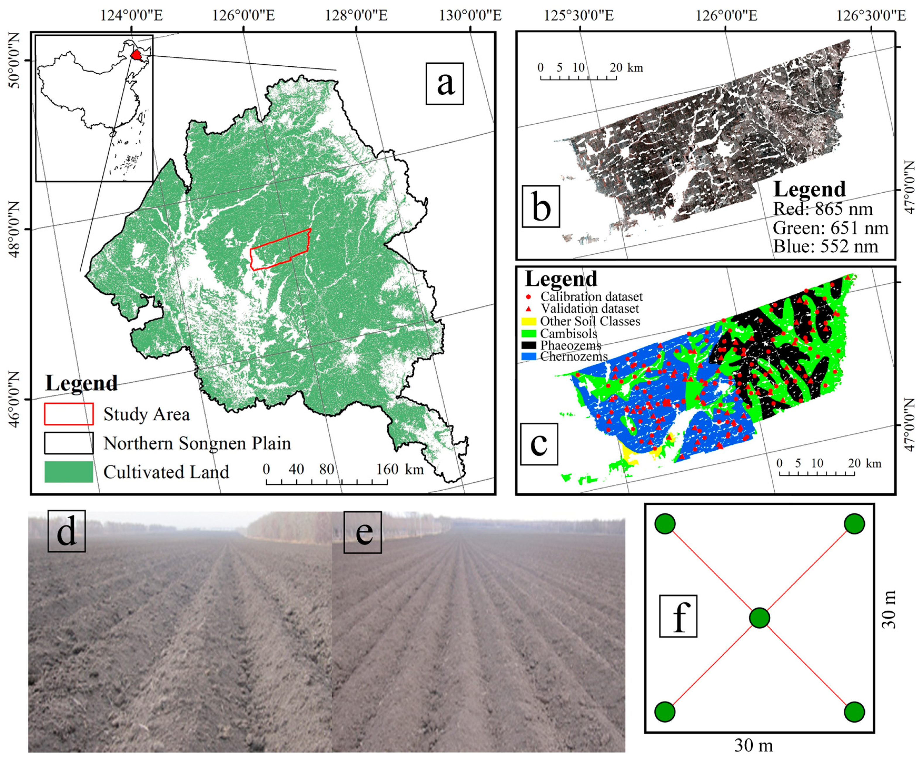
2.1. Study Area

MingShui County is located in the north of the Songnen Plain, southwest of Heilongjiang Province (Figure 1a). It covers the area of 124°18′–125°21′ E, 46°44′–47°29′ N. The study area is the cultivated land area of Mingshui county. The total area is approximately 1481 km², with an average elevation of 249.2 m. The eastern part of the study area is located in the Xiaoxing’an Mountains, and the western part is located in the hinterland of the Songnen Plain. The elevation gradually decreases from the middle to the eastern and western sides. The annual average temperature is approximately 2.9 °C, and the annual average precipitation is approximately 480 mm. Figure 1c is the Second National Soil Survey map, which is the great group level according to the Genetic Soil Classification of China. The map was obtained from http://vdb3.soil.csdb.cn/, accessed on 1 June 2020. The map was produced in the 1980s, and it was produced by the government by digging out and analyzing the soil profile. The scale of the map is 1:1,000,000. The study area includes Phaeozems, Chernozems and Cambisols, according to the World Reference Base for Soil Resources (Figure 1c). Phaeozems and Chernozems have higher SOM contents and good water-holding capacities. Different from Phaeozems, the surface layer of Chernozems has a calcic horizon. Cambisols primarily occur in relatively low-lying areas dispersed among the other soil classes. The study area is called the black soil region by local people because the surface of soil appears black, and the topsoil of the region is covered with black or dark humus. The soil in the black soil region is clayey soil; thus, the difference in soil pH and texture is small, with little influence on the prediction results.

The study area is dominated by annual vegetation, and the farmers in this area deal with crop residues (such as straw) with the traditional burning method, which hardly leaves any residue in the cultivated land. The cultivated land is plowed from the end of March to the end of April each year, and then the cultivated soil is directly exposed to the surface. At the time of study, there is no vegetation and snow cover on the soil surface (Figure 1d,e). There is neither a large area of vegetation nor a large area of snow cover, as April and May occur in the “bare soil period” [38].

2.2. Data Acquisition and Treatment

2.2.1. Soil Sample Collection and Treatment

A total of 166 topsoil samples (0–20 cm) were collected in the study area, and soil samples were taken along the main roads to ensure that the sampling points were covered on different soil classes (Figure 1c). Each topsoil sample is composed of 5–6 subsamples that are selected from a 30 × 30 m square (Figure 1f), and the 30 × 30 m squares align with the pixels of the satellite images. Thus, the measured SOM content represents the average value in the area. The center coordinates of each topsoil sample grid are recorded by a portable global positioning system (GPS, G350, UniStrong, Beijing, China). Each soil sample is put into a cloth bag to facilitate soil storage and prevent soil cross-contamination. In the laboratory, each soil sample is air-dried, ground, and sieved to sizes of ≤2 mm [39], and then the SOM content is determined by the potassium dichromate method [40].

2.2.2. GF-5 Hyperspectral Data Acquisition and Treatment

GF-5 hyperspectral data were requested and downloaded from the China Center for Resources Satellite Data and Application (http://www.cresda.com/CN/, accessed on 5 June 2019) (Figure 1b). The spatial resolution is 30 m, the swath width is 60 km, and the spectral range is from 390 to 2513 nm, with a total of 330 spectral bands. Among them, there are 150 bands in the visible and near-infrared range (390–1000 nm), the spectral resolution is 4.28 nm, and there are 180 bands with a spectral resolution of 8.42 nm in the shortwave infrared range (1000–2513 nm). The ranges of 390–430 and 2450–2513 nm have low signal-to-noise ratios, and the sensor is affected by the sensor interface at 900–1050 nm and atmospheric water vapor absorption at 1350–1451 and 1771–1982 nm, resulting in discontinuous spectral data. Therefore, the ranges of 430–900, 1050–1350, 1451–1771 and 1982–2450 nm are selected as the spectral ranges of this study. We acquired four cloud-free hyperspectral images, and the acquired dates were 3 April, 10 April and 12 April 2019. The acquired dates are consistent with the “bare soil period”. There was no rainfall in the week before we obtained the hyperspectral data; therefore, the soil surface was relatively dry. There is no obvious stripe noise in the image, and the image quality is good. The images were radiometrically calibrated to eliminate sensor error and determine the accurate radiation value at the entrance of the sensor, caused by atmospheric attenuation with radiometric calibration. The images are atmospherically corrected to eliminate the influence of the solar angle on the spectral reflectance of surface objects during the different periods, and the radiation error caused by Fast Line-of-Sight Atmospheric Analysis of Spectral Hypercubes (FLAASH) modules in the Environment for Visualizing Images (ENVI) version 5.3 (Harris Geospatial Corporation, Boulder, CO, USA) software, and then geometric precision correction was carried out for the image to ensure that the offset was small and corresponded to the ground sampling points. This way, there is almost no radiation and atmospheric correction noise in the image; thus, our methods mainly focus on specific sensor noise.

2.3. Fractional-Order Derivatives (FOD)

As a conventional preprocessing algorithm, derivative technology can enhance the peak valley change in the spectral curve, eliminate the influence of the baseline translation and linear rotation, and weaken the background noise, enhancing the spectral characteristics and improving the prediction accuracy of the soil properties [41,42]. Compared with integer-order derivatives, FODs are helpful when capturing the changes in spectral reflectance details and have strong application potential in visible, near-infrared soil spectral analysis [43]. Of the commonly used definitions of the FOD, the Grünwald Letnikov (G-L) definition is appropriate for spectral reflectance processing, due to its computational simplicity [44].

The function of the first derivative is described as follows

$$f^{\prime }(x)=\underset{h\to 0}{lim}\frac{f(x+h)-f(x)}{h}$$

(1)

where $f\left(x\right)$ is the reflectance of the xth band and h is the increment of the xth band. The function of the second derivative is described as follows

$$f^{″}(x)=\underset{h\to 0}{lim}\frac{f(x+2h)-2f(x+h)+f(x)}{h^2}$$

(2)

If the derivative order changes from an integer to a fraction (v), the v-order derivative function in the interval of [a, b], based on the G-L function, can be described as follows

$$d^{(v)}f(x)=\underset{h\to 0}{lim}\frac{1}{h^v}{\displaystyle \sum _{m=0}^{[(b-a)/h]}{(-1)}^m\frac{\Gamma (v+1)}{m!\Gamma (v-m+1)}}f(x-mh)$$

(3)

where [(b − a)/h] is the integer part of (b − a)/h and h is the step length. The Gamma function is described as follows

$$\Gamma (z)={\displaystyle {\int }_0^{\infty }exp(-u)u^{z-1}du=(z-1)}!$$

(4)

Then, Equation (3) can be described as follows

$$\frac{d^{v}f(x)}{d{x}^v}\approx f(x)+(-v)f(x-1)+\frac{(-v)(-v+1)}{2}f(x-2)+\cdots \frac{\Gamma (-v+1)}{m!\Gamma (-v+m+1)}f(x-m)$$

(5)

Equation (5) is used to calculate eleven FODs, increasing from 0 to 2 with a 0.2 step length in MATLAB R2016b (MathWorks, Natick, MA, USA). The 0-order, 1-order and 2-order derivatives represent the original reflectance (OR), first derivatives and second derivatives, respectively.

2.4. Denoising Methods

2.4.1. Singular Value Decomposition (SVD)

SVD is a commonly used linear decomposition method. A singular value is regarded as the representative value of the matrix to reflect all the matrix information. SVD can map the original data to a low-dimensional space, to complete data compression and noise reduction, and has been used in the field of image noise reduction [45] and signal restoration [46], which has the advantages of less phase shift and no delay.

In the construction of the Hankel matrix (H_m) of the spectral reflectance signal, H_m is a matrix of m*n, and the decomposition function of H_m can be described as follows

$$H_m=U\Sigma V^{*}$$

(6)

where U and V are m*m and n*n unitary matrices, respectively, V^* is the conjugate transpose of V, and Σ is a m*n positive semidefinite matrix. When there is noise in the signal, H_m is a nonsingular matrix. The following relation occurs among the singular values after decomposition

$${\sigma }_1>{\sigma }_2>{\sigma }_3>\cdots >{\sigma }_k>{\sigma }_{k+1}>\cdots >{\sigma }_n$$

(7)

where ${\sigma }_k$ is the kth singular value obtained by SVD, which is also represented as a demarcation point in the noisy signal. Thus, the k singular values contain the signal energy, and the subsequent singular value corresponds to the noise component in the signal [47]; a larger singular value contains more original information.

2.4.2. Fourier Transform (FT)

FT is one of the most fundamental algorithms in the area of signal processing and can transform a signal from the time domain to a different frequency domain. The transformed frequency domain components can be transformed back to the time domain by inverse FT [48,49]. For satellite hyperspectral data, FT has been used to transform the spectral signal to different frequency domain components, where the high-frequency component contains most of the noise in the hyperspectral data [50]. Inverse FT is the superposition of complex sinusoidal components with frequencies ranging from zero to infinity, and the adequacy of the basis functions gains in expression from the few high-magnitude coefficients required in the representation. The FT function can be described as follows

$$F(\omega )=F^{\prime }[f(t)]={\displaystyle {\int }_{-\infty }^{\infty }f(t)e^{-iwt}dt}$$

(8)

where F(ω) is the image function of f(t) and f(t) is the image primitive function of F(ω). All the mathematical procedures used in the spectral data for decomposition, time domain transformation and frequency domain transformation are implemented within the R open-source environment.

2.4.3. Discrete Wavelet Transform (DWT)

The DWT samples the scale and translation of a continuous wavelet based on an integer power of 2. Compared with the continuous wavelet transform [51,52], the DWT is more suitable for signal and image denoising and compression, especially for nonlinear or nonstationary signals [53]. The method decomposes the original spectral data into wavelet coefficients, analyzes the variation rules of the wavelet coefficients, and reconstructs the spectral data. The DWT includes signal decomposition and signal reconstruction. In signal decomposition, the original spectral data are decomposed into high-frequency and low-frequency information based on the signal length and wavelet basis length. The high-frequency information is mainly composed of noise, and the low-frequency information is the wavelet coefficient. Each scale decomposes the low-frequency information of the upper scale until the maximum scale of decomposition is reached. At decomposition scale j, low-frequency information Aj and high-frequency information Dj are present. Therefore, the original spectral data S are the sum of the low-frequency information at the final scale J and high-frequency information at all scales j = 1, …, J (Equation (9)) [54].

$$S=A_J+{\displaystyle {\sum }_{j\le J}{D}_j}$$

(9)

In signal reconstruction, the low-frequency information of each scale is reconstructed to obtain the spectral data of each scale after reconstruction. In this paper, we test a few mother wavelet functions and select the ‘db4’ mother wavelet.

2.5. Optimal Band Combination Algorithm

The optimal band combination algorithm constructs the spectral index by calculating the correlation between the combination of different bands and SOM content, which is helpful for improving the prediction accuracy of soil properties. In this paper, we extract the DI, RI, NDI, renormalized difference index (RDVI) and modified simple ratio (MSR) (

Table 1. A summary of the set of spectral indexes used in this study.

Spectral Index and Formula	Literature
$DI(R_i,R_j)=R_i-R_j$	[35]
$RI(R_i,R_j)=\frac{R_i}{R_j}$	[35]
$NDI(R_i,R_j)=\frac{R_i-R_j}{R_i+R_j}$	[35]
$RDVI(R_i,R_j)=\frac{R_i-R_j}{\sqrt{R_i+R_j}}$	[54,55]
$MSR(R_i,R_j)=\frac{R_i}{R_j}-1/\sqrt{\frac{R_i}{R_j}+1}$	[56,57]

Note: R_i and R_j represent the bands selected from 430–900, 1050–1350, 1451–1771 and 1982–2450 nm. The spectral indexes are constructed from the OR and FODs, respectively. The process of constructing the spectral indexes is implemented in MATLAB R2016b.

).

2.6. Recursive Feature Elimination (RFE)

In this paper, the independent variables of the model include the spectral reflectance and spectral indexes. RFE can prevent model overfitting caused by too many independent variables, reduce the complexity, and improve the prediction accuracy and calculation efficiency of the model [58]. The RFE algorithm uses a rudimentary model for multiple rounds of training, and the basic model selected in this paper is the random forest model. After each round of training, the independent variables are scored according to the coefficient of each independent variable, and the independent variable with the smallest score is removed. Then, a new set of independent variables is constructed with the remaining independent variables for the next round of training until all the independent variables have been traversed [59]. In this paper, the whole-soil samples are divided into calibration and validation datasets at a 2:1 scale, the 10-fold cross validation method and the calibration dataset are used to determine the optimal number of independent variables, and the corresponding independent variables are selected as the input of SOM prediction.

2.7. Random Forest (RF)

The RF algorithm proposed by Breiman et al. [60] and Cutler et al. [61] is an integrated model composed of multiple decision trees that are not related to each other. The specific steps of RF algorithm are as follows:

(1)

Samples are randomly selected from the calibration set, and then each sample is used to build a decision tree;

(2)

Each split node in the decision tree is randomly selected from n inputs, such that the variable space can be completely divided;

(3)

The final result of the RF model is the average value of the predicted results of all decision trees.

The number of decision trees (ntree), minimum number of blades (nodesize) and number of variables randomly sampled as candidates for each split (mtry) should be set when establishing the RF prediction model. The greater ntree, the more stable the RF model [62]. Thus, we set ntree = 500. The value of mtry is one-third of the total number of inputs [6]. The value of nodesize is determined by repeated testing. We set the minimum value of nodesize as 1 and the maximum value as no more than the number of independent variables. After repeated tests, the optimal value of nodesize is determined. In this paper, the RF model is established by using the “randomForest” package in the R software [63].

2.8. Model Calibration and Validation

In this paper, soil samples are arranged in the order of SOM content, ranging from small to large, and then the whole-soil samples are divided into calibration and validation datasets at a 2:1 scale; thus, there are 111 soil samples in calibration and 55 soil samples in validation datasets. To compare the prediction performance of different denoising methods, we calculate several statistical parameters from the laboratory-measured results and predicted results based on the validation and calibration sets. These parameters include the coefficient of determination (R²), the root mean square error (RMSE) and the ratio of performance to interquartile range (RPIQ). In general, a well-performing model should have a high R² and RPIQ and low RMSE. The calculation formulas of the above parameters are as follows

$$R^2=1-\frac{{\displaystyle {\sum }_{i=1}^n{(y_i-{\widehat{y}}_i)}^2}}{{\displaystyle {\sum }_{i=1}^n{(y_i-{\overline{y}}_i)}^2}}$$

(10)

$$RMSE=\sqrt{\frac{1}{n}{\displaystyle {\sum }_{i=1}^n{(y_i-{\widehat{y}}_i)}^2}}$$

(11)

$$RPIQ=\frac{IQ}{RMSE}$$

(12)

where n is the number of soil samples, y_i is the laboratory-measured SOM content of sample i, ${\widehat{y}}_i$ is the predicted SOM content of soil sample i, $\overline{y}$ is the average SOM content of the whole-soil sample, IQ is the interquartile range (IQ = Q3 − Q1) of the observed values, Q1 is the first quartile and Q3 is the third quartile.

3. Results

3.1. Description of Soil Samples

The descriptive statistics of the SOM contents are shown in

Table 2. Statistical descriptions of the SOM contents on the whole, calibration and validation datasets.

Set	N	Max (g kg−1)	Min (g kg−1)	Mean (g kg−1)	SD (g kg−1)	CV (%)
Whole dataset	166	56.30	26.10	40.81	6.55	16.10
Calibration dataset	111	56.30	26.10	40.90	6.76	16.53
Validation dataset	55	55.80	26.20	40.64	6.11	15.03

Note: N represents the number of soil samples. Max, Min, SD and CV represent the maximum value, minimum value, standard deviation and coefficient of variation of SOM content in a dataset, respectively.

. On the whole dataset, the SOM content exhibited a wide range from 26.10 to 56.30 g kg⁻¹, with a mean value of 40.81 g kg⁻¹, an SD of 6.55 g kg⁻¹, and a CV of 16.10%. Compared with the CV of the whole dataset, the CV of the calibration dataset is higher and that of the validation dataset is lower.

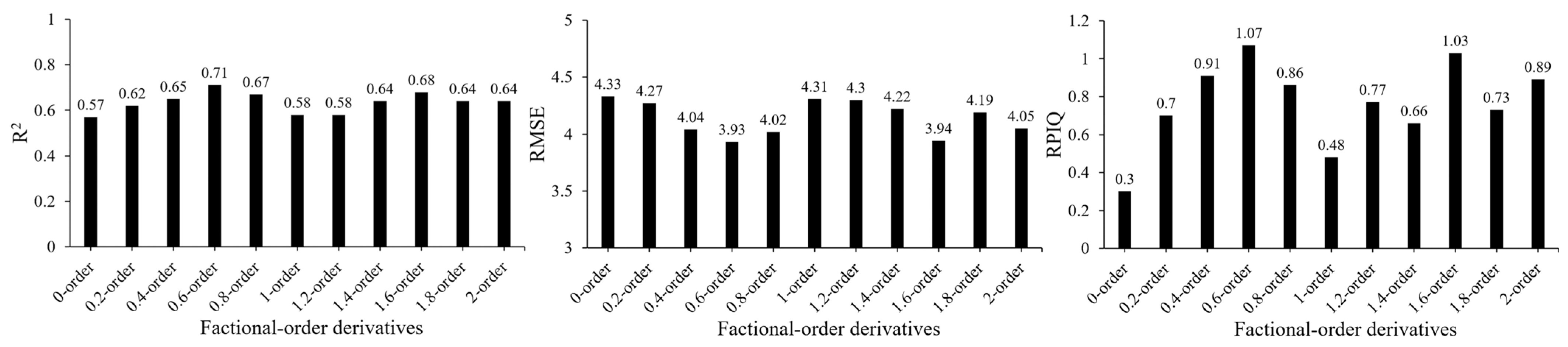
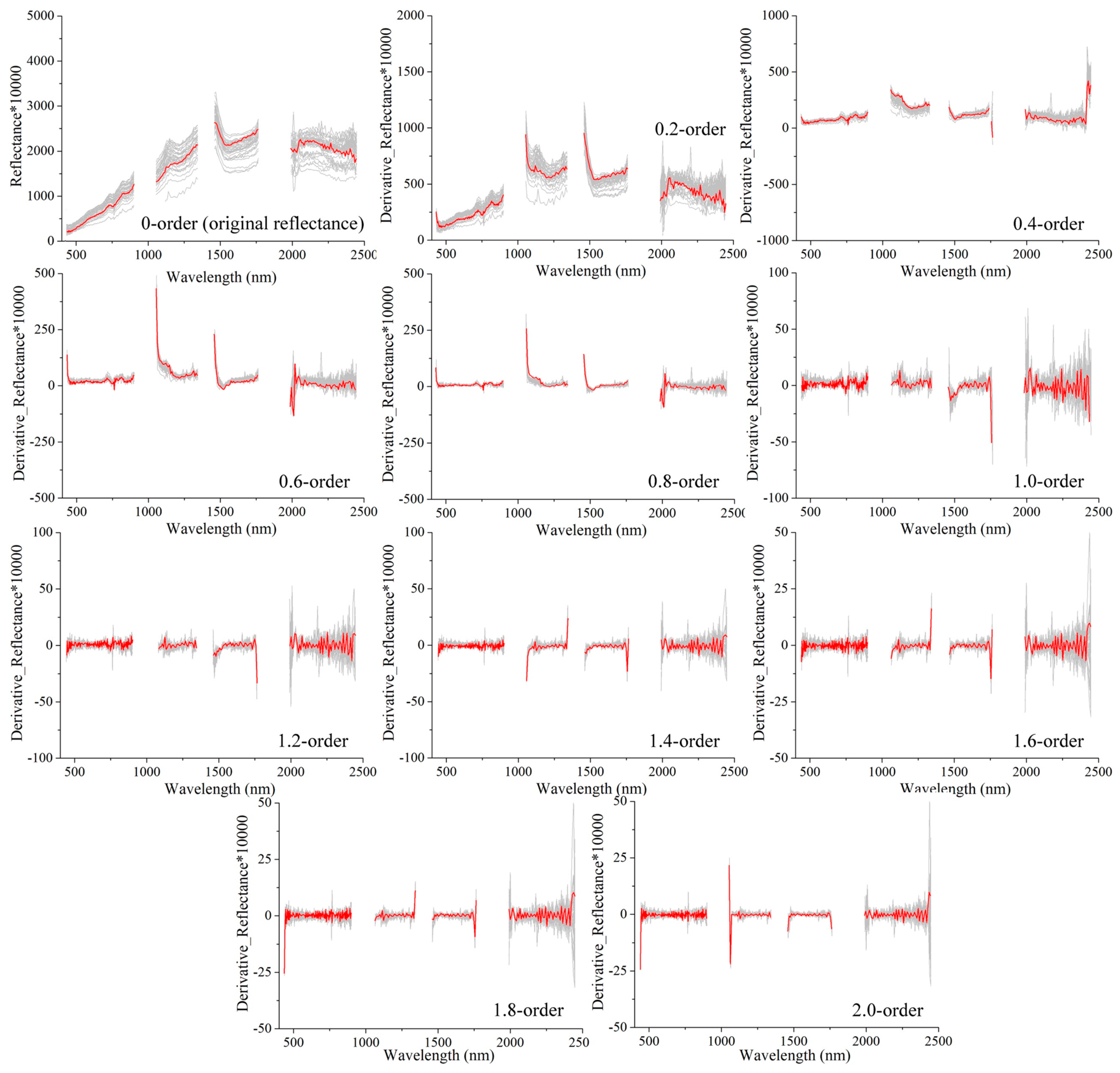
3.2. Selected Optimal FOD

We evaluate the SOM predictions from the satellite hyperspectral data under different FODs, and the accuracy bar chart shows that the SOM prediction accuracy can be improved by the FOD (Figure 2). Under different FODs, the prediction accuracy of the FODs is higher than that of integer-order derivatives (1-order and 2-order). Overall, the prediction accuracy of order > 1 is lower than that of order < 1, and the highest prediction accuracy is achieved by the 0.6-order derivative (R² = 0.71, RMSE = 3.93 g kg⁻¹, RPIQ = 1.07). Therefore, in this paper, the optimal FOD is 0.6-order, and a further analysis is made on the basis of 0.6-order FOD.

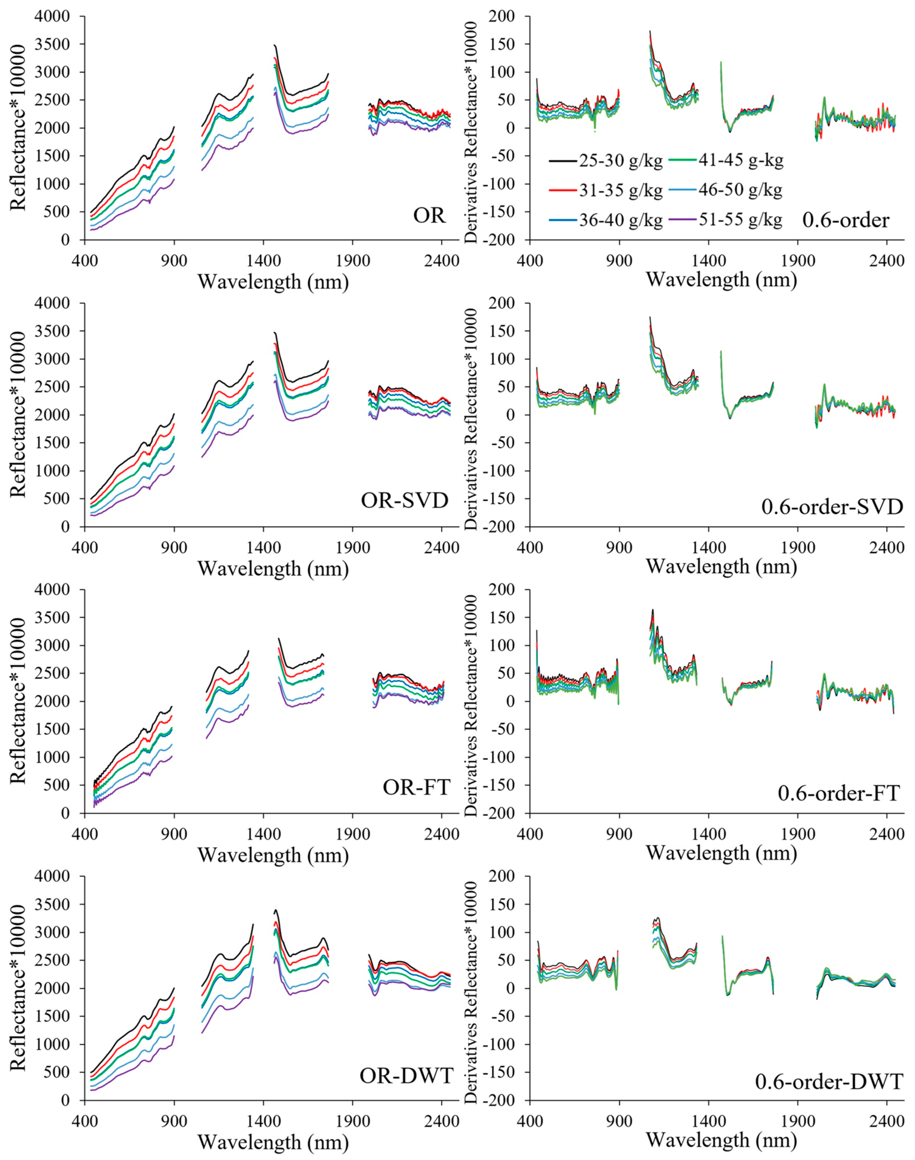
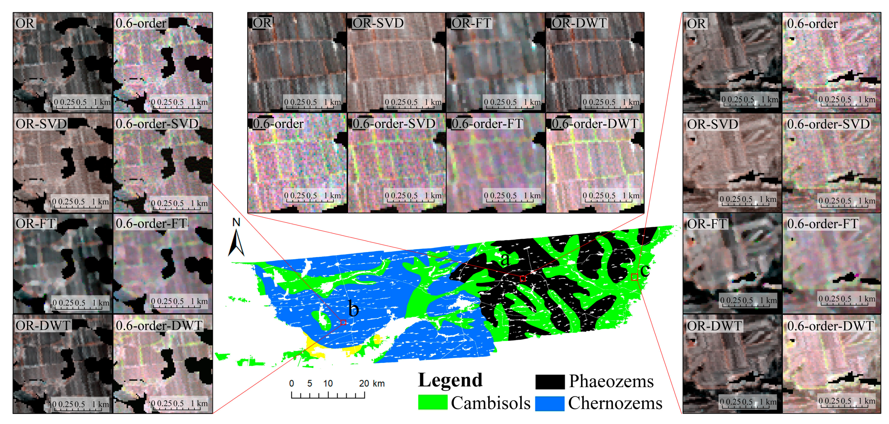
3.3. Spectral Characteristics of Different Denoising Methods

The soil spectral reflectance curves extracted from satellite hyperspectral images of different SOM content under different denoising methods are shown in Figure 3. As a whole, the reflectance decreases with increasing SOM content, and the shapes of the soil spectral reflectance curves with different SOM contents are similar [64]. With OR-SVD, OR-FT and OR-DWT, the spectral reflectance curves still retain the spectral characteristics of the OR, and the spectral reflectance curve becomes smoother, which effectively reduces the noise in the reflectance data, especially at the edges of the spectral range (1700–1800, 2000–2100 and 2400–2450 nm).

With the 0.6-order reflectance, most of the processed reflectance values across the whole vis-NIR region gradually approach 0, which proves that the baseline drifts and overlapping peaks are removed. Under different denoising methods at 0.6-order reflectance, the noise in the spectral data is significantly reduced. With the 0.6-order-SVD, the noise above 2000 nm is obviously reduced. With the 0.6-order-FT, the detailed information in the spectral curve is amplified, for example, at approximately 1500 and 2000 nm. With the 0.6-order-DWT, the small “burr” shape in the curve is reduced, the absorption characteristics become more obvious, and the difference in the spectral curves with different SOM contents is obvious at 430–600 nm.

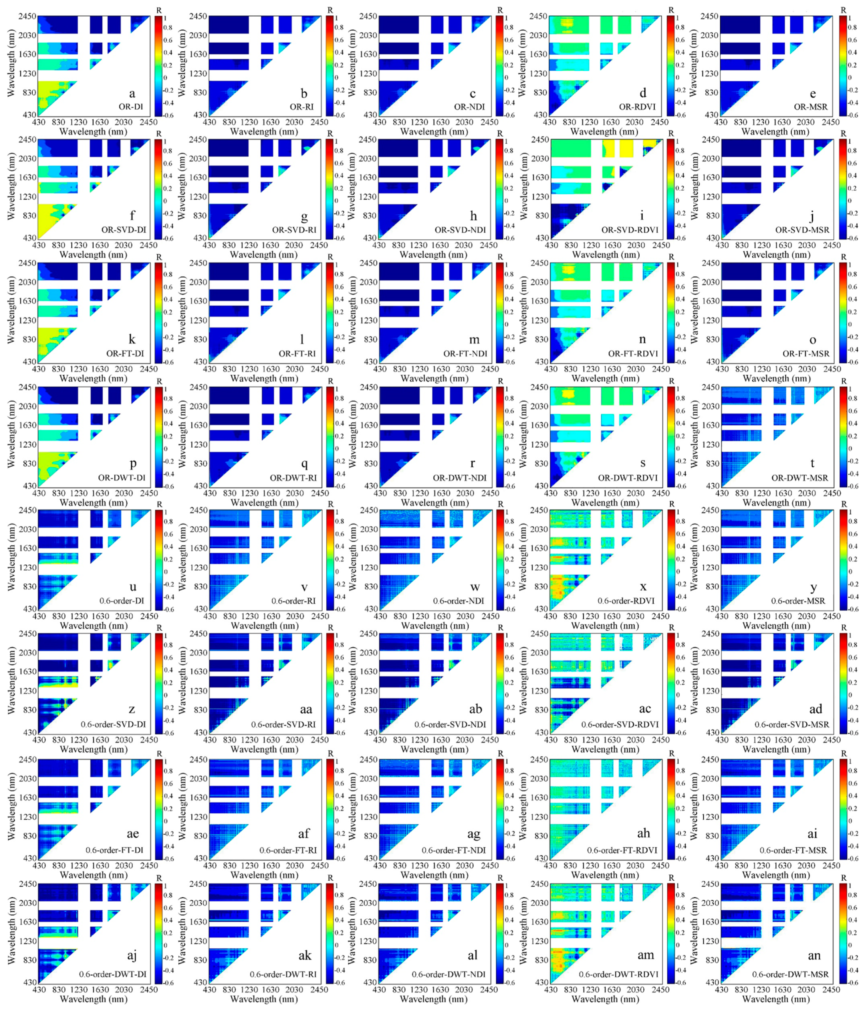
3.4. Optimal Band Combination Algorithm

The correlations between the DI, RI, NDI, RDVI, MSR and SOM contents for different denoising methods are shown in Figure 4. In different spectral indexes, RI, RDVI, and MSR have higher correlations with the SOM content. For a certain denoising method, the 0.6-order reflectance has a higher correlation than the OR, and the distribution pattern of the correlation coefficient becomes finer. Therefore, the 0.6-order can capture detailed spectral information of SOM.

The optimal bands of different spectral indexes are shown in

Table 3. The correlations between SOM content and the optimal DI, RI, NDI, RDVI and MSR.

Denoising Method	DI		RI		NDI		RDVI		MSR
	Bands	R	Bands	R	Bands	R	Bands	R	Bands	R
OR	R805, R775	0.55 **	R2412, R741	−0.57 **	R822, R771	−0.55 **	R565, R557	−0.61 **	R2412, R527	−0.57 **
OR-SVD	R531, R514	0.59 *	R2311, R548	−0.61 **	R544, R540	0.61 **	R2252, R1114	0.60 **	R2311, R548	−0.61 **
OR-FT	R771, R651	0.59 **	R2412, R527	−0.62 **	R450, R441	0.61 **	R1350, R651	−0.62 **	R2412, R488	−0.61 **
OR-DWT	R882, R771	0.58 **	R2226, R766	−0.61 **	R818, R771	−0.58 **	R2066, R1131	0.62 **	R2218, R762	−0.61 **
0.6-order	R1072, R822	0.59 **	R1468, R433	−0.63 **	R1468, R1433	−0.62 **	R570, R753	−0.70 **	R1468, R433	−0.64 **
0.6-order-SVD	R2024, R1072	−0.60 **	R514, R454	−0.62 **	R493, R454	−0.63 **	R2201, R843	0.64 **	R514, R454	0.67 **
0.6-order-FT	R1603, R886	−0.64 **	R1721, R685	−0.65 **	R1721, R445	−0.62 **	R578, R749	−0.77 **	R1721, R685	−0.65 **
0.6-order-DWT	R2176, R890	−0.64 **	R2066, R441	−0.65 **	R2074, R433	−0.62 **	R574, R835	−0.77 **	R2066, R441	−0.64 **

Note: R₈₀₅ represents the band at 805 nm, * represents significant value at the 0.01 < p < 0.05 level, and ** represents significant value at the p < 0.01 level.

. Under different denoising methods, the correlation between spectral indexes and SOM contents is obviously different. With OR-SVD and 0.6-order-SVD, the best bands of different spectral indexes are always in the visible and near infrared range (454, 493, 514, 531, 843 and 1114 nm). With 0.6-order-DWT, the highest R is achieved. The bands at 441, 574, 890, 2066 and 2176 nm are selected multiple times, and thus are particularly important for the prediction of SOM.

3.5. Selection of the Input Variables

The selected input variables after RFE for the different denoising methods are shown in

Table 4. Selection of the input variables based on the RFE method.

Denoising Method	Input Variables
OR	R1485, R1511, RI, NDI, RDVI, MSR
OR-SVD	R1485, R1536, RI, NDI, MSR
OR-FT	DI, RI, NDI, RDVI, MSR
OR-DWT	RI, NDI, RDVI, MSR
0.6-order	R488, R531, RI, NDI, MSR
0.6-order-SVD	R598, DI, NDI, RDVI, MSR
0.6-order-FT	DI, RI, NDI, RDVI, MSR
0.6-order-DWT	DI, RI, NDI, RDVI

. The input variables of the different denoising methods yield obvious discrepancies; most of the variables are spectral indexes, and NDI is always selected. With OR, OR-SVD, OR-FT and OR-DWT, the input variables are composed of spectral indexes and some single bands of around 1500 nm. With 0.6-order, 0.6-order-SVD, 0.6-order-FT and 0.6-order-DWT, the input variables are composed of spectral indexes and some single bands of around 500 nm. Compared with OR, the selected wavelengths and optimal wavelength in different spectral indexes always shift towards the visible range after 0.6-order derivatives (Table 3 and Table 4).

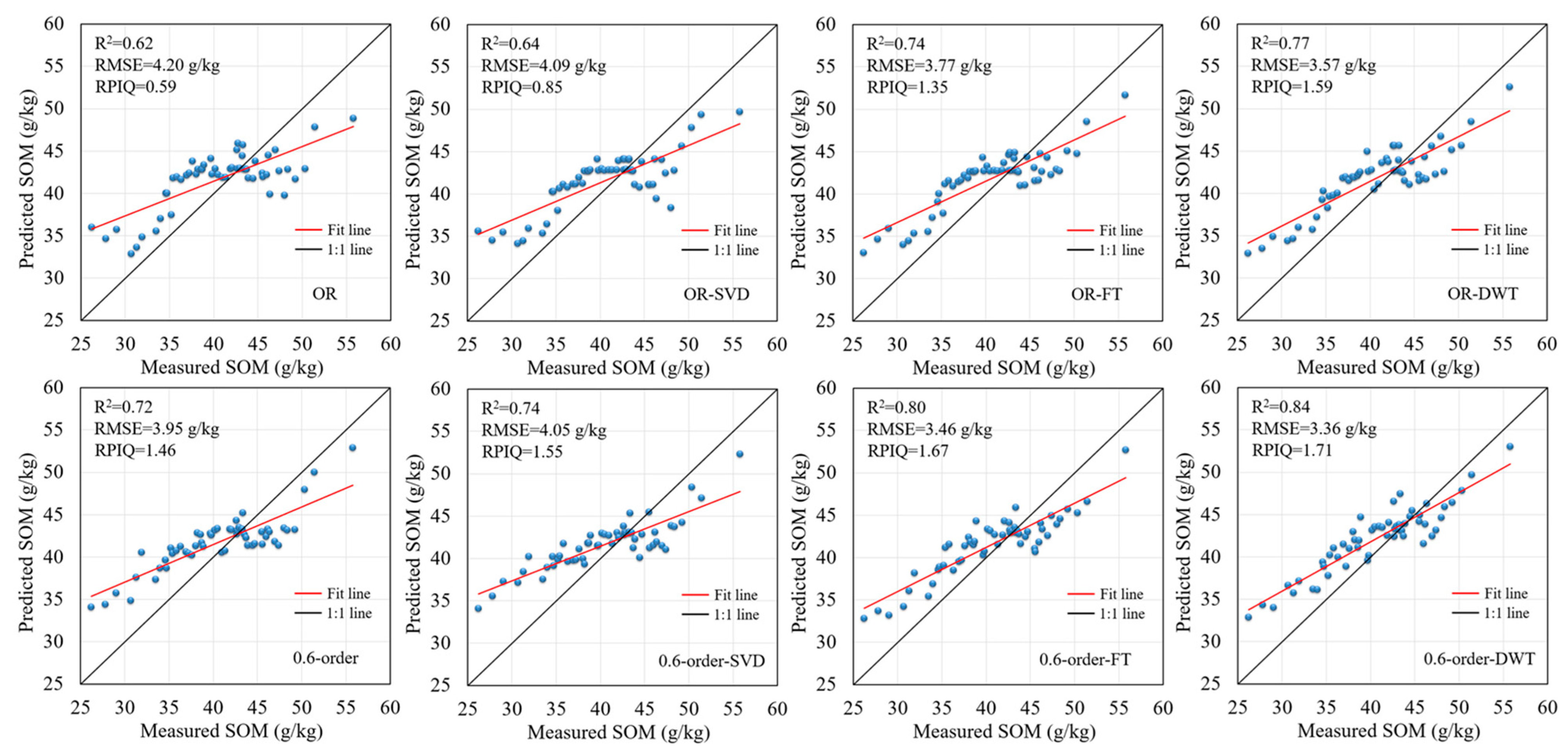
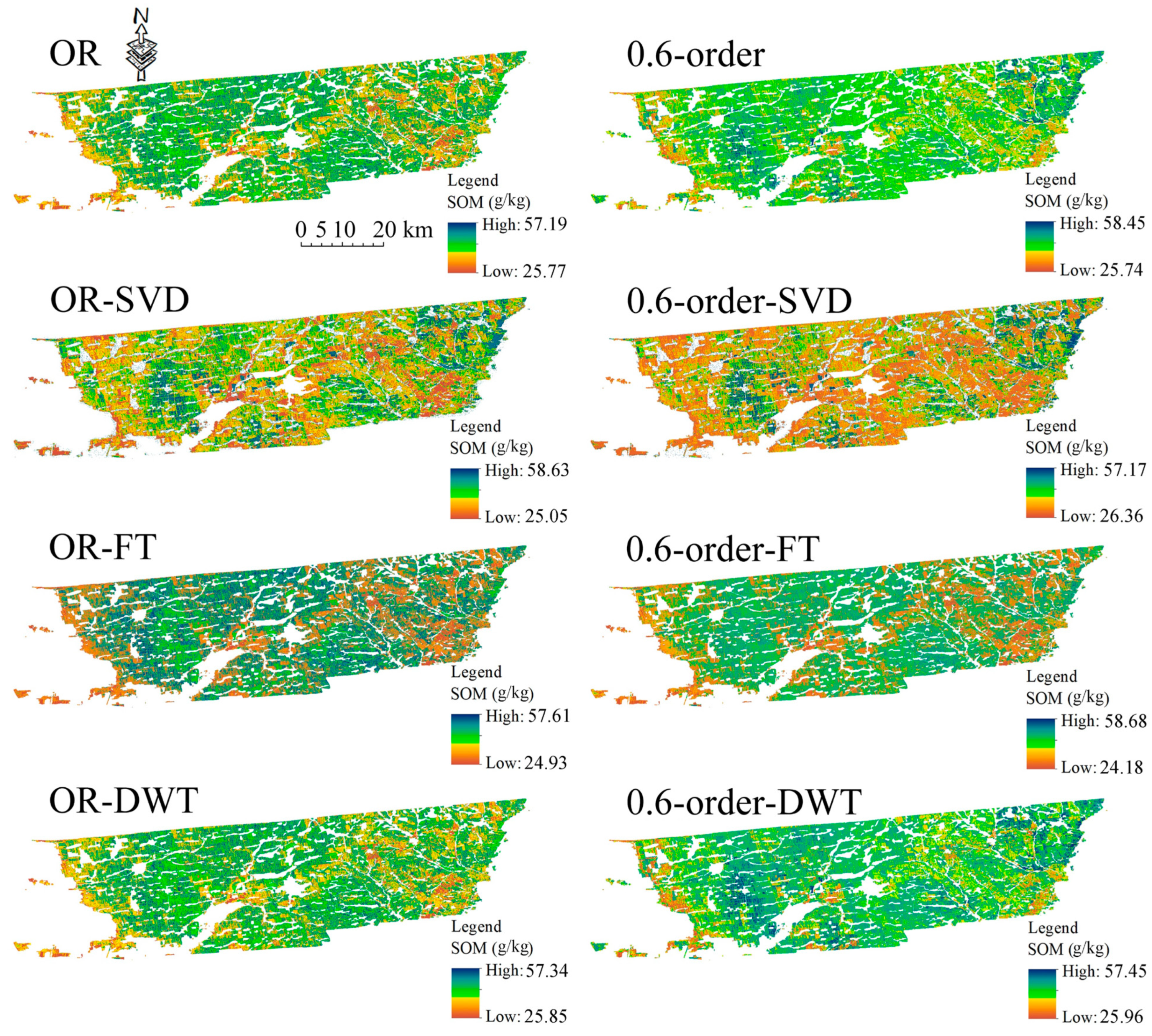
3.6. Prediction Accuracy and Spatial Distribution of SOM

The SOM prediction results of the RF prediction model are combined with the input variables after RFE (Figure 5). Compared with that by OR (R² = 0.62, RMSE = 4.20 g kg⁻¹ and RPIQ = 0.59), the SOM prediction accuracy can be improved by using different denoising methods. OR-SVD is less effective in improving the SOM prediction accuracy. OR-FT and OR-DWT can greatly improve the SOM prediction accuracy. The prediction accuracy of OR-DWT is the highest (R² = 0.77, RMSE = 3.57 g kg⁻¹, RPIQ = 1.59). With the 0.6-order reflectance, the SOM prediction accuracy can be further improved under different denoising methods. The highest prediction accuracy is achieved by 0.6-order-DWT (R² = 0.84, RMSE = 3.36 g kg⁻¹, RPIQ = 1.71). Compared with those of OR, the R² and RPIQ of 0.6-order-DWT are 22% and 1.12 higher, and the RMSE is 0.84 g kg⁻¹ lower.

The maps of the SOM spatial distribution under different denoising methods are shown in Figure 6. With OR-SVD and 0.6-order-SVD, the predicted SOM spatial distribution value is relatively low. Overall, the spatial distribution of SOM content is similar under different denoising methods. The SOM content in the middle of the study area is high, while that in the southwest and southeast is low. The SOM content in the eastern part of the study area is high, largely due to the Phaeozems and flat terrain in this area, and Phzeozems has high soil fertility (Figure 5). The middle of the study area is condu cive to the accumulation of calcareous components and the formation of a calcareous layer, because the soil is easily affected by groundwater, the surface soil has sufficient soil-forming conditions for humus to be preserved and gradually thickened, and the soil class is mainly Chernozems, meaning that the SOM content in the middle of the study area is relatively high. In the southwestern and southeastern parts of the study area, the elevation is low, and erosion is serious, which hinders the accumulation of SOM; the soil class is mainly Cambisols. The spatial distribution of SOM content is basically consistent with that of soil classes.

4. Discussion

4.1. Advantages of the Fractional-Order Derivative Method

The spectral derivative is a powerful mathematical tool to address the problem of multiple collinearity problems and has a strong influence on the peak in the microspectrum [2,65,66]. Compared with the integer-order derivative (first derivatives and second derivatives), the order of the FOD is extended from integer order to noninteger order, which can extract more detailed spectral information for SOM prediction from satellite hyperspectral data (Figure 7). The SOM prediction accuracy first increases and then decreases with increasing order (Figure 2), which may be due to the increase in order; the deformation of the absorption valley and absorption peak in the spectral curve increases gradually, and the noise in the spectral data also increases gradually. Therefore, a high-order FOD may have unfavorable effects on the processing of satellite hyperspectral data. For instance, on the 0.6-order scale (Figure 7), the spectral curve retains some of the obvious absorption peaks and absorption valleys of the OR, and the curve is relatively smooth, especially at 430–600 and 2200–2450 nm. After 0.6-order (Figure 7), with increasing order, there are no significant discrepancies in the spectral curves of different SOM contents, and the spectral characteristics are weakened, especially at 600–800, 1200–1400 and 1500–1750 nm. The spectral curves almost become a straight line, and the spectral noise at the end of the spectral region (800–900, 2300–2450 nm) is gradually amplified.

In this paper, we used the FOD to extract spectral details from satellite hyperspectral data for the first time and determine that the optimal order of the FOD in satellite hyperspectral data is the 0.6-order, which is lower than the optimal order of airborne hyperspectral data (0.75-order) and laboratory-measured hyperspectral data (1.25-order) [2,43,67]. This is mainly due to the presence of more noise in satellite hyperspectral data. Compared with previous studies [67,68,69], we use a smaller step length (0.2), so that we can more precisely analyze the variation in different order derivatives and extract more spectral details from the satellite hyperspectral data.

4.2. Comparation on the Performances of Different Denoising Methods

To show the spectral characteristics of different soil classes under different denoising methods, images of the center locations of different soil classes were shown in Figure 8. The location a, b and c of Figure 8 representing the images of Phaeozems, Chernozems and Cambisols, respectively. The overall image color from SVD is significantly different from those from other denoising methods, and the contrast between different soil classes is reduced. OR-DWT has higher similarity to OR in color and characteristics, while OR-FT weakens the characteristics in some parts. Both FT and DWT can greatly improve the SOM prediction accuracy, and DWT has higher accuracy (Figure 5), because FT and DWT can concentrate the information of abrupt changes in reflectance and interference noise in the high-frequency region, concentrate the information of the parts with a flat reflectance in the original image in the low-frequency region, and then retain low-frequency information for reconstruction [70]. FT uses large waves, while DWT uses small waves [71]. Similar to FT’s transformation, which of time domain signals into triangle functions, DWT decomposes signals into different scale components [72], and the resolution in the time and frequency domains is linked to the type of base function used for transformation. The resolution expands (or contracts) according to a scale factor and is temporally shifted along the entire definition range of the signal. Therefore, we can remove the noise from the signal while retaining the essential signal features; that is, the wavelet transform concentrates the signal features into a few large-magnitude wavelet coefficients. The process preserves the spectral information and eliminates the noise information, and DWT is better at processing nonstationary signals (reflectance).

The image details of the 0.6-order reflectance and OR significantly differ (Figure 8). In general, the ‘salt and pepper’ characteristics of the 0.6-order-SVD image are obvious, and the image characteristics of different soil classes are weaker. The SOM prediction accuracy is slightly better after SVD, because the hyperspectral data become several uncorrelated singular values after SVD processing. The singular values are arranged from large to small, and the reduction in singular values decreases particularly quickly. In many cases, the sum of the first 10% or even 1% singular values accounts for more than 90% of the total information of the OR. According to the first 10% or even 1% singular values, the inverse operation is carried out to obtain the hyperspectral data after noise reduction [73]. However, this process not only reduces the noise, but also loses some of the OR information, resulting in the SOM prediction accuracy being slightly improved. In the comparison of 0.6-order-FT with 0.6-order-DWT, the spatial characteristics of 0.6-order-DWT are more obvious. Therefore, in the study of soil property prediction, it is necessary to adopt certain noise reduction methods to increase the contrast between different soil classes.

4.3. Discrepancies between Spectral Indexes of Laboratory-Measured and Satellite Hyperspectral Data

The spectral index is constructed according to the correlation between the combination of any two bands and the SOM content. In general, the two selected bands in different spectral indexes are different. Even for the same spectral index, the selected bands are different, due to different hyperspectral data sources (laboratory-measured, airborne and satellite) and different processing methods. With the OR-DWT, the highest correlation between the selected bands and SOM appears at 750–900, 1131 and 2226 nm, and the correlation is approximately −0.61^** (Table 3). With the 0.6-order-DWT, the selected bands with the highest correlation appear at 400–600 and 2100 nm; the correlation is approximately −0.66^** (Table 3). Compared with the sensitive bands between the laboratory-measured hyperspectral data and SOM content (600–800, 1200 nm) [74], the sensitive bands between the satellite hyperspectral data and SOM content occur in the range of visible light, especially after the FOD processing.

NDI, DI and RI are commonly used for SOM prediction [35,75]. We extract more spectral indexes from the satellite hyperspectral data to better develop and utilize spectral information and proved that these spectral indexes have good applicability in SOM prediction.

4.4. Advantages of Recursive Feature Elimination

The RFE algorithm has been widely used in medical diagnosis and mineral element mapping [76,77]. We try to use this method to process a large number of spectral data and spectral indexes and prove that the SOM prediction accuracy can be improved with RFE. Compared with the prediction accuracy of the full spectrum as input variables in OR (R² = 0.57, RMSE = 4.33 g kg⁻¹, RPIQ = 0.30), that of the selected input variables after RFE is better (R² = 0.62, RMSE = 4.20 g kg⁻¹, RPIQ = 0.59) (Figure 2 and Figure 5). The method has the following advantages. First, the model can reduce the redundant information in hyperspectral data and effectively improve the computational efficiency of the model. Second, the algorithm directly discriminates the optimal set of input variables through the prediction accuracy. Compared with the method of selecting the input variables according to the correlation, the model established in this paper can simplify the analysis process of SOM prediction, be more easily transformed for subsequent practical applications and be applied to remote sensing satellites for regional-scale SOM prediction. Finally, compared with the principal component analysis commonly used in previous research [5,78], RFE can retain the physical meaning of input, which is helpful for better understanding the relationship between the input and changes in SOM content [79].

4.5. The Uncertainty Analysis

The laboratory-measured hyperspectral data contain low noise and easily yield high-accuracy SOM predictions. However, it is difficult to map the spatial distribution of SOM content on a large scale. To realize the dynamic monitoring of SOM content on a large scale, satellite data are needed. In view of the noise information in satellite hyperspectral data, three different denoising methods are selected in this paper to compare the potential of different denoising methods in SOM prediction and to map the spatial distribution of SOM content. However, our experiment cannot fully identify and eliminate the noise in hyperspectral images because the resolution of hyperspectral satellite data in different spectral ranges varies, and existing satellite hyperspectral data cannot provide a reference for correction. In future studies, we plan to combine satellite hyperspectral data with laboratory-measured hyperspectral data because the spectral interval of 1 nm of the laboratory-measured spectral curve may help us to fully correct the potential error information in the satellite hyperspectral data. In addition, as an important factor affecting soil organic matter inversion, field management should be taken into consideration in future research.

5. Conclusions

In this paper, the optimal FOD of satellite hyperspectral data was determined, three denoising methods were compared to improve the SOM content prediction accuracy, and the spatial distribution of the SOM content was mapped. The main outcomes were as follows: (1) the FOD can improve the SOM content prediction accuracy, as FODs have more advantages than integer-order derivatives, and high-order derivatives may have unfavorable effects on satellite hyperspectral data. With different FODs, the highest prediction accuracy was achieved by 0.6 orders (R² = 0.71, RMSE = 3.93 g kg⁻¹, RPIQ = 1.07), because the 0.6-order spectral curve still retains some of the obvious absorption peak and absorption valley of original reflectance, and the curve is relatively smooth. (2) The correlation coefficients between the five extracted spectral indexes and SOM content passed the significance test at the 0.01 level. Compared with the SOM-sensitive bands of laboratory-measured hyperspectral data, the selected bands of different spectral indexes occured more in the range of visible light. (3) The selected input variables after the RFE algorithm were mainly spectral indexes. RFE can simplify the analysis process of SOM prediction and is more easily applied to remote-sensing satellites for regional-scale SOM prediction. (4) Both denoising methods can improve the SOM content prediction accuracy; the accuracies of the different denoising methods were ranked DWT > FT > SVD, and the highest prediction accuracy was achieved by 0.6-order-DWT (R² = 0.84, RMSE = 3.36 g kg⁻¹, RPIQ = 1.71).

This paper confirmed the influence of different denoising methods on SOM content prediction from satellite hyperspectral data, improved the application level of satellite hyperspectral data in soil remote sensing and constructed a reliable regional-scale SOM prediction model.

References

1. Luo, Z.K.; Wang, E.L.; Sun, O.J. Soil carbon change and its responses to agricultural practices in Australian agro-ecosystems: A review and synthesis. Geoderma 2010, 155, 211–223. [Google Scholar] [CrossRef]
2. Wang, X.P.; Zhang, F.; Kung, H.T.; Johnson, V.C. New methods for improving the remote sensing estimation of soil organic matter content (SOMC) in the Ebinur Lake Wetland National Nature Reserve (ELWNNR) in northwest China. Remote Sens. Environ. 2018, 218, 104–118. [Google Scholar] [CrossRef]
3. Nocita, M.; Stevens, A.; Wesemael, B.V.; Aitkenhead, M.; Bachmann, M.; Barthès, B. Soil spectroscopy: An alternative to wet chemistry for soil monitoring. Adv. Agron. 2015, 132, 139–159. [Google Scholar] [CrossRef]
4. Roudier, P.; Hedley, C.B.; Lobsey, C.R.; Viscarra Rossel, R.A.; Leroux, C. Evaluation of two methods to eliminate the effect of water from soil vis-NIR spectra for predictions of organic carbon. Geoderma 2017, 296, 98–107. [Google Scholar] [CrossRef]
5. Liu, S.S.; Shen, H.H.; Chen, S.C.; Zhao, X.; Biswas, A.; Jia, X.L.; Shi, Z.; Fang, J.Y. Estimating forest soil organic carbon content using vis-NIR spectroscopy: Implications for large-scale soil carbon spectroscopic assessment. Geoderma 2019, 348, 37–44. [Google Scholar] [CrossRef]
6. Meng, X.T.; Bao, Y.L.; Liu, J.G.; Liu, H.J.; Zhang, X.L.; Zhang, Y.; Wang, P.; Tang, H.T.; Kong, F.C. Regional soil organic carbon prediction model based on a discrete wavelet analysis of hyperspectral satellite data. Int. J. Appl. Earth Obs. Geoinf. 2020, 89, 102111. [Google Scholar] [CrossRef]
7. Clark, R.N.; King, T.V.V.; Klejwa, M.; Swayze, G.; Vergo, N. High spectral resolution reflectance spectroscopy of minerals. J. Geophys. Res. 1990, 4, 12653–12680. [Google Scholar] [CrossRef] [Green Version]
8. Bendor, E.; Banin, A. Near-infrared analysis as a rapid method to simultaneously evaluate several soil properties. Soil Sci. Soc. Am. J. 1995, 59, 364–372. [Google Scholar] [CrossRef]
9. Barnes, E.M.; Sudduth, K.A.; Hummel, J.W.; Lesch, S.M.; Corwin, D.L.; Yang, C.; Daughtry, C.S.T.; Bausch, W.C. Remote-and ground-based sensor techniques to map soil properties. Photogramm. Eng. Remote Sens. 2003, 69, 619–630. [Google Scholar] [CrossRef] [Green Version]
10. Bao, Y.L.; Meng, X.T.; Ustin, S.; Wang, X.; Zhang, X.L.; Liu, H.J.; Tang, H.T. Vis-SWIR spectral prediction model for soil organic matter with different grouping strategies. Catena 2020, 195, 104703. [Google Scholar] [CrossRef]
11. Lucà, F.; Conforti, M.; Castrignanò, A.; Matteucci, G.; Buttafuoco, G. Effect of calibration set size on prediction at local scale of soil organic carbon by Vis-NIR spectroscopy. Geoderma 2017, 288, 175–183. [Google Scholar] [CrossRef]
12. Selige, T.; Böhner, J.; Schmidhalter, U. High resolution topsoil mapping using hyperspectral image and field data in multivariate regression modelling procedures. Geoderma 2006, 136, 235–244. [Google Scholar] [CrossRef]
13. Stevens, A.; Wesemael, B.; Vandenschrick, G.; Touré, S.; Tychon, B. Detection of carbon stock change in agricultural soils using spectroscopic techniques. Soil Sci. Soc. Am. J. 2006, 70, 844–850. [Google Scholar] [CrossRef]
14. Wang, J.; He, T.; Lv, C.; Chen, Y.; Jian, W. Mapping soil organic matter based on land degradation spectral response units using Hyperion images. Int. J. Appl. Earth. Obs. Geoinf. 2010, 12, S171–S180. [Google Scholar] [CrossRef]
15. Shi, P.; Castaldi, F.; Wesemael, B.; Van Oost, K. Large-scale, high-resolution mapping of soil aggregate stability in croplands using APEX hyperspectral imagery. Remote Sens. 2020, 12, 666. [Google Scholar] [CrossRef] [Green Version]
16. Mirik, M.; Norland, J.E.; Crabtree, R.L.; Biondini, M.E. Hyperspectral one-meter-resolution remote sensing in Yellowstone National Park, Wyoming: I. Forage nutritional values. Rangel. Ecol. Manag. 2005, 58, 452–458. [Google Scholar] [CrossRef]
17. Zhang, T.T.; Li, L.; Zheng, B.Z. Estimation of agricultural soil properties with imaging and laboratory spectroscopy. J. Appl. Remote Sens. 2013, 7, 073587. [Google Scholar] [CrossRef]
18. Demarchi, L.; Chan, J.C.W.; Ma, J.L.; Canters, F. Mapping impervious surfaces from superresolution enhanced CHRIS/Proba imagery using multiple endmember unmixing. ISPRS J. Photogramm. 2012, 72, 99–112. [Google Scholar] [CrossRef]
19. Wang, C.C.; Xue, R.R.; Zhao, S.H.; Liu, S.H.; Wang, X.; Li, H.Z.; Liu, Z.Q. Quality evaluation and analysis of GF-5 hyperspectral image data. Geogr. Geo-Inf. Sci. 2021, 37, 33–39. (In Chinese) [Google Scholar]
20. Bendor, E.; Gila, N. A simple indicator for estimating the noise level of a hyperspectral data cube for earth observation missions. Acta Astronaut. 2016, 128, 304–312. [Google Scholar] [CrossRef]
21. Yu, W.B.; Zhang, M.; Shen, Y. Learning a local manifold representation based on improved neighborhood rough set and LLE for hyperspectral dimensionality reduction. Signal Process. 2019, 164, 20–29. [Google Scholar] [CrossRef]
22. Goyal, B.; Dogra, A.; Agrawal, S.; Sohi, B.S.; Sharma, A. Image denoising review: From classical to state-of-the-art approaches. Inf. Fusion 2020, 55, 220–244. [Google Scholar] [CrossRef]
23. Nawar, S.; Buddenbaum, H.; Hill, J.; Kozak, J.; Mouazen, A.M. Estimating the soil clay content and organic matter by means of different calibration methods of vis-NIR diffuse reflectance spectroscopy. Soil Tillage Res. 2016, 155, 510–522. [Google Scholar] [CrossRef] [Green Version]
24. Guo, L.; Zhao, C.; Zhang, H.T.; Chen, Y.Y.; Linderman, M.; Zhang, Q.; Liu, Y.L. Comparisons of spatial and non-spatial models for predicting soil carbon content based on visible and near-infrared spectral technology. Geoderma 2017, 285, 280–292. [Google Scholar] [CrossRef]
25. Dotto, A.C.; Dalmolin, R.S.D.; Caten, A.T.; Grunwald, S. A systematic study on the application of scatter-corrective and spectral-derivative preprocessing for multivariate prediction of soil organic carbon by Vis-NIR spectra. Geoderma 2018, 314, 262–274. [Google Scholar] [CrossRef]
26. Gao, J.L.; Meng, B.P.; Liang, T.G.; Feng, Q.S.; Ge, J.; Yin, J.P.; Wu, C.X.; Cui, X.; Hou, M.J.; Liu, J.; et al. Modeling alpine grassland forage phosphorus based on hyperspectral remote sensing and a multi-factor machine learning algorithm in the east of Tibetan Plateau, China. ISPRS J. Photogramm. 2019, 147, 104–117. [Google Scholar] [CrossRef]
27. Gholizadeh, A.; Boruvka, L.; Saberioon, M.M.; Kozak, J.; Vasat, R.; Nemecek, K. Comparing different data preprocessing methods for monitoring soil heavy metals based on soil spectral features. Soil Water Res. 2015, 10, 218–227. [Google Scholar] [CrossRef] [Green Version]
28. Wang, F.H.; Gao, J.; Zha, Y. Hyperspectral sensing of heavy metals in soil and vegetation: Feasibility and challenges. ISPRS J. Photogramm. 2018, 136, 73–84. [Google Scholar] [CrossRef]
29. Yu, C.Y.; Sun, J.Y. Signal separation from X-ray image sequence using singular value decomposition. Biomed. Signal Process. Control 2018, 42, 210–215. [Google Scholar] [CrossRef]
30. Chandrakasan, A.; Gutnik, V.; Xanthopoulos, T. Data driven signal processing: An approach for energy efficient computing. Int. Symp. Low Power Electron. Des. 1996, 19, 347–352. [Google Scholar]
31. Zhang, C.; Zhou, L.; Zhao, Y.Y.; Zhu, S.S.; Liu, F.; He, Y. Noise reduction in the spectral domain of hyperspectral images using denoising autoencoder methods. Chemom. Intell. Lab. Syst. 2020, 203, 104063. [Google Scholar] [CrossRef]
32. Mishra, P.; Karami, A.; Nordon, A.; Rutledge, D.N.; Roger, J.M. Automatic de-noising of close-range hyperspectral images with a wavelength-specific shearlet-based image noise reduction method. Sens. Actuators B-Chem. 2019, 42, 210–215. [Google Scholar] [CrossRef]
33. Zhu, L.; Zhang, S.; Zhao, H.; Chen, S.; Wei, D.; Lu, X. Classification of UAV-to-Ground Vehicles Based on Micro-Doppler Signatures Using Singular Value Decomposition and Deep Convolutional Neural Networks. IEEE Access 2019, 7, 22133–22143. [Google Scholar] [CrossRef]
34. Zhang, G.W.; Peng, S.L.; Cao, S.Y.; Zhao, J.; Xie, Q.; Han, Q.J.; Wu, Y.F.; Huang, Q.B. A fast progressive spectrum denoising combined with partial least squares algorithm and its application in online Fourier transform infrared quantitative analysis. Anal. Chim. Acta 2019, 1074, 62–68. [Google Scholar] [CrossRef] [PubMed]
35. Hong, Y.S.; Chen, S.C.; Chen, Y.Y.; Linderman, M.; Mouazen, A.M.; Liu, Y.L.; Guo, L.; Yu, L.; Liu, Y.F.; Cheng, H.; et al. Comparing laboratory and airborne hyperspectral data for the estimation and mapping of topsoil organic carbon: Feature selection coupled with random forest. Soil. Tillage Res. 2020, 199, 104589. [Google Scholar] [CrossRef]
36. Jin, X.L.; Du, J.; Liu, H.J.; Wang, Z.M.; Song, K.S. Remote estimation of soil organic matter content in the Sanjiang Plain, Northest China: The optimal band algorithm versus the GRA-ANN model. Agric. For. Meteorol. 2016, 218–219, 250–260. [Google Scholar] [CrossRef]
37. Souza, A.B.; Demattê, J.A.M.; Fellipe, A.O.; Mello, F.A.O.; Salazar, D.F.U.; Mendes, W.S.; Safanelli, J.L. Ratio of Clay Spectroscopic Indices and its approach on soil morphometry. Geoderma 2020, 357, 113963. [Google Scholar] [CrossRef]
38. Yang, H.X.; Zhang, X.K.; Xu, M.Y.; Shao, S.; Wang, X.; Liu, W.Q.; Wu, D.Q.; Ma, Y.Y.; Bao, Y.L.; Zhang, X.L.; et al. Hyper-temporal remote sensing data in bare soil period and terrain attributes for digital soil mapping in the Black soil regions of China. Catena 2020, 184, 104259. [Google Scholar] [CrossRef]
39. O’Kelly, B.C. Accurate determination of moisture content of organic soils using the oven drying method. Dry. Technol. 2004, 22, 1767–1776. [Google Scholar] [CrossRef]
40. Nelson, D.W.; Sommers, L. A rapid and accurate procedure for estimation of organic carbon in soils. Proc. Indiana Acad. Sci. 1975, 84, 456–462. [Google Scholar]
41. Vašát, R.; Kodešová, R.; Klement, A.; Borůvka, L. Simple but efficient signal pre-processing in soil organic carbon spectroscopic estimation. Geoderma 2017, 298, 46–53. [Google Scholar] [CrossRef]
42. Stavroulakis, P.I.; Liatsis, P.; Tipping, N.; Craddock, P. Evaluation and Optimization of the Savitzky-Golay Smoothing Filter for Noise Reduction in Thin Film Interference Signal Analysis; Harvard University Press: Cambridge, MA, USA, 2013. [Google Scholar]
43. Hong, Y.S.; Liu, Y.L.; Chen, Y.Y.; Liu, Y.F.; Yu, L.; Liu, Y.; Cheng, H. Application of fractional-order derivative in the quantitative estimation of soil organic matter content through visible and near-infrared spectroscopy. Geoderma 2019, 337, 758–769. [Google Scholar] [CrossRef]
44. Tian, D.; Xue, D.Y.; Wang, D.H. A fractional-order adaptive regularization primal-dual algorithm for image denoising. Inf. Sci. 2015, 296, 147–159. [Google Scholar] [CrossRef]
45. Devi, H.S.; Singh, K.M. Red-cyan anaglyph image watermarking using DWT, Hadamard transform and singular value decomposition for copyright protection. J. Inf. Secur. Appl. 2020, 50, 102424. [Google Scholar] [CrossRef]
46. Yao, L.L.; Yuan, C.J.; Qiang, J.J.; Feng, S.T.; Nie, S.P. Asymmetric color image encryption based on singular value decomposition. Opt. Laser Eng. 2017, 89, 80–87. [Google Scholar] [CrossRef]
47. Xu, X.B.; Luo, M.Z.; Tan, Z.Y.; Pei, R.H. Echo signal extraction method of laser radar based on improved singular value decomposition and wavelet threshold denoising. Infrared Phys. Technol. 2018, 92, 327–335. [Google Scholar] [CrossRef]
48. Banas, K.; Banas, A.M.; Heussler, S.P.; Breese, M.B.H. Influence of spectral resolution, spectral range and signal-to-noise ratio of Fourier transform infra-red spectra on identification of high explosive substances. Spectrochim. Acta A 2018, 188, 106–112. [Google Scholar] [CrossRef]
49. Yang, L.; Song, M.; Zhu, A.X.; Qin, C.Z.; Zhou, C.H.; Qi, F.; Li, X.M.; Chen, Z.Y.; Gao, B.B. Predicting soil organic carbon content in croplands using crop rotation and Fourier transform decomposed variables. Geoderma 2019, 340, 289–302. [Google Scholar] [CrossRef]
50. Iwen, M.A. Combinatorial Sublinear-Time Fourier Algorithms. Found. Comput. Math. 2010, 10, 303–338. [Google Scholar] [CrossRef]
51. Zhang, J.; Rivard, B.; Sanchez-Azofeifa, G.A.; Castro, K. Intra and inter-class spectral variability of tropical tree speciesat La Selva, Costa Rica: Implicationsfor species identification using HYDICE imagery. Remote Sens. Environ. 2006, 105, 129–141. [Google Scholar] [CrossRef]
52. Cheng, T.; Rivard, B.; Sanchez-Azofeifa, G.A. Spectroscopic determination of leaf water content using continuous wavelet analysis. Remote Sens. Environ. 2011, 115, 659–670. [Google Scholar] [CrossRef]
53. Joy, J.J.; Santhi, N.; Ramar, K.; Bama, B.S. Spatial frequency discrete wavelet transform image fusion technique for remote sensing applications. Eng. Sci. Technol. 2019, 22, 715–726. [Google Scholar] [CrossRef]
54. Blackburn, G.A. Wavelet decomposition of hyperspectral data: A novel approach to quantifying pigment concentrations in vegetation. Int. J. Remote Sens. 2007, 28, 2831–2855. [Google Scholar] [CrossRef]
55. Roujean, J.; Breon, F. Estimating PAR absorbed by vegetation from bidirectional reflectance measurements. Remote Sens. Environ. 1995, 51, 375–384. [Google Scholar] [CrossRef]
56. Baret, F.; Guyot, G. Potentials and limits of vegetation indices for LAI and APAR assessment. Remote Sens. Environ. 1991, 35, 161–173. [Google Scholar] [CrossRef]
57. Chen, J.M. Evaluation of vegetation indices and a modified simple ratio for boreal applications. Can. J. Remote Sens. 1996, 22, 229–242. [Google Scholar] [CrossRef]
58. Yan, K.; Zhang, D. Feature selection and analysis on correlated gas sensor data with recursive feature elimination. Sens. Actuators B-Chem. 2015, 212, 353–363. [Google Scholar] [CrossRef]
59. You, W.J.; Yang, Z.J.; Ji, G.L. Feature selection for high-dimensional multi-category data using PLS-based local recursive feature elimination. Expert Syst. Appl. 2014, 41, 1463–1475. [Google Scholar] [CrossRef]
60. Breiman, L. Random forests. Mach. Learn. 2001, 45, 5–32. [Google Scholar] [CrossRef] [Green Version]
61. Cutler, A.; Stevens, J.R. Random forests for microarrays. Methods Enzymol. 2006, 422–432. [Google Scholar] [CrossRef]
62. Díaz-Uriarte, R.; Andrés, S.A.D. Gene selection and classification of microarray data using random forest. BMC Bioinform. 2006, 7, 3–16. [Google Scholar] [CrossRef] [PubMed] [Green Version]
63. Liaw, A.; Wiener, M. Classification and regression by randomForest. R News 2002, 2, 18–22. [Google Scholar]
64. Lucà, F.; Conforti, M.; Matteucci, G.; Buttafuoco, G. Prediction of organic carbon and nitrogen in forest soil using visible and near-infrared spectroscopy. EAGE Near Surf. Geosci. 2015, 2015, 1–5. [Google Scholar] [CrossRef]
65. Wang, Z.; Zhang, X.L.; Zhang, F.; Chan, N.W.; Kung, H.Y.; Liu, S.H.; Deng, L.F. Estimation of soil salt content using machine learning techniques based on remote-sensing fractional derivatives, a case study in the Ebinur Lake Wetland National Nature Reserve, Northwest China. Ecol. Indic. 2020, 119, 106869. [Google Scholar] [CrossRef]
66. Li, B.; Xie, W. Adaptive fractional differential approach and its application to medical image enhancement. Comput. Electr. Eng. 2015, 45, 324–335. [Google Scholar] [CrossRef]
67. Hong, Y.S.; Guo, L.; Chen, S.C.; Linderman, M.; Mouazem, A.M.; Yu, L.; Chen, Y.Y.; Liu, Y.L.; Liu, Y.F.; Cheng, H.; et al. Exploring the potential of airborne hyperspectral image for estimating topsoil organic carbon: Effects of fractional-order derivative and optimal band combination algorithm. Geoderma 2020, 365, 114228. [Google Scholar] [CrossRef]
68. Kougioumtzoglou, I.A.; Santos, K.R.M.D.; Comerfoed, L. Incomplete data based parameter identification of nonlinear and time-variant oscillators with fractional derivative elements. Mech. Syst. Signal. Process. 2017, 94, 279–296. [Google Scholar] [CrossRef]
69. Abulaiti, Y.; Sawut, M.; Maimaitiaili, B.; Ma, C. A possible fractional order derivative and optimized spectral indices for assessing total nitrogen content in cotton. Comput. Electron. Argic. 2020, 171, 105275. [Google Scholar] [CrossRef]
70. Reis, M.S.; Saraiva, P.M.; Bakshi, B.R. Denoising and Signal-to-Noise Ratio Enhancement: Wavelet Transform and Fourier Transform. Compr. Chemom. 2009, 25–55. [Google Scholar] [CrossRef]
71. Reju, R.A.; Kgabi, N.A. Wavelet analyses and comparative denoised signals of meteorological factors of the namibian atmosphere. Atmos. Res. 2018, 213, 537–549. [Google Scholar] [CrossRef]
72. Dai, X.P.; Cheng, L.Z.; Mareschal, J.C.; Lemire, D.; Liu, C. New method for denoising borehole transient electromagnetic data with discrete wavelet transform. J. Appl. Geophys. 2019, 168, 41–48. [Google Scholar] [CrossRef]
73. Yadav, J.; Sehra, K. Large Scale Dual Tree Complex Wavelet Transform based robust features in PCA and SVD subspace for digital image water marking. Procedia Comput. Sci. 2018, 132, 863–872. [Google Scholar] [CrossRef]
74. Shepherd, K.D.; Walsh, M.G. Development of reflectance spectral libraries for characterization of soil properties. Soil. Sci. Soc. Am. J. 2002, 66, 988–998. [Google Scholar] [CrossRef]
75. Bao, N.S.; Wu, L.X.; Ye, B.Y.; Yang, K.; Zhou, W. Assessing soil organic matter of reclaimed soil from a large surface coal mine using a field spectroradiometer in laboratory. Geoderma 2017, 288, 47–55. [Google Scholar] [CrossRef]
76. Bustamam, A.; Bachiar, A.; Sarwinda, D. Selecting Features Subsets Based on Support Vector Machine-Recursive Features Elimination and One Dimensional-Naïve Bayes Classifier using Support Vector Machines for Classification of Prostate and Breast Cancer. Procedia Comput. Sci. 2019, 157, 450–458. [Google Scholar] [CrossRef]
77. Richhariya, B.; Tanveer, M.; Rashid, A.H. Diagnosis of Alzheimer’s disease using universum support vector machine based recursive feature elimination (USVM-RFE). Biomed. Signal Process. 2020, 59, 101903. [Google Scholar] [CrossRef]
78. Shi, Z.; Ji, W.J.; Viscarra Rossel, R.A.; Chen, S.C.; Zhou, Y. Prediction of soil organic matter using a spatially constrained local partial least squares regression and the Chinese vis-NIR spectral library. Eur. J. Soil Sci. 2015, 66, 679–687. [Google Scholar] [CrossRef]
79. Wang, C.B.; Pan, Y.P.; Chen, J.G.; Ouyang, Y.P.; Rao, J.F.; Jiang, Q.B. Indicator element selection and geochemical anomaly mapping using recursive feature elimination and random forest methods in the Jingdezhen region of Jiangxi Province, South China. Appl. Geochem. 2020, 122, 104760. [Google Scholar] [CrossRef]
Figure 1. Overview of the study area: (a) northern Songnen Plain map; (b) GF-5 hyperspectral image; (c) soil sampling location and soil classes; (d,e) photographs of the soil surface of cultivated land after plowing; (f) sampling with the five-point method.
Remotesensing 13 02273 g001
Figure 2. With increasing from 0 to 2 with a 0.2 step length, prediction accuracy of the laboratory-measured versus predicted SOM contents from the validation dataset in the RF prediction model with the full spectrum as input variables.
Remotesensing 13 02273 g002
Figure 3. Spectral reflectance curves under different denoising methods. Note: OR represents the original reflectance. OR-SVD, OR-FT, OR-DWT and 0.6-order represents the reflectance after singular value decomposition, fourier transform, discrete wavelet transform and 0.6-order derivatives processing, respectively. 0.6-order-SVD, 0.6-order-FT and 0.6-order-DWT represents the 0.6-order reflectance after singular value decomposition, fourier transform and discrete wavelet transform processing, respectively.
Remotesensing 13 02273 g003
Figure 4. Established optimal spectral indexes under different denoising methods. Note: OR-DI represents the difference index of the OR, OR-SVD-DI represents the difference index of the reflectance after SVD processing, 0.6-order-SVD-DI represents the difference index of the 0.6-order reflectance after SVD, etc.
Remotesensing 13 02273 g004
Figure 5. Scatter plots of the laboratory-measured versus predicted SOM contents from the validaTable 1. line, and the red solid lines represent the regression line.
Remotesensing 13 02273 g005
Figure 6. Maps of the SOM spatial distributions under different denoising methods.
Remotesensing 13 02273 g006
Figure 7. Varying spectral curves of the whole dataset under different FODs (0 to 2, increment of 0.2). The red curve represents the average spectral curve of the whole dataset.
Remotesensing 13 02273 g007
Figure 8. Images of the different soil classes under different denoising methods.
Remotesensing 13 02273 g008