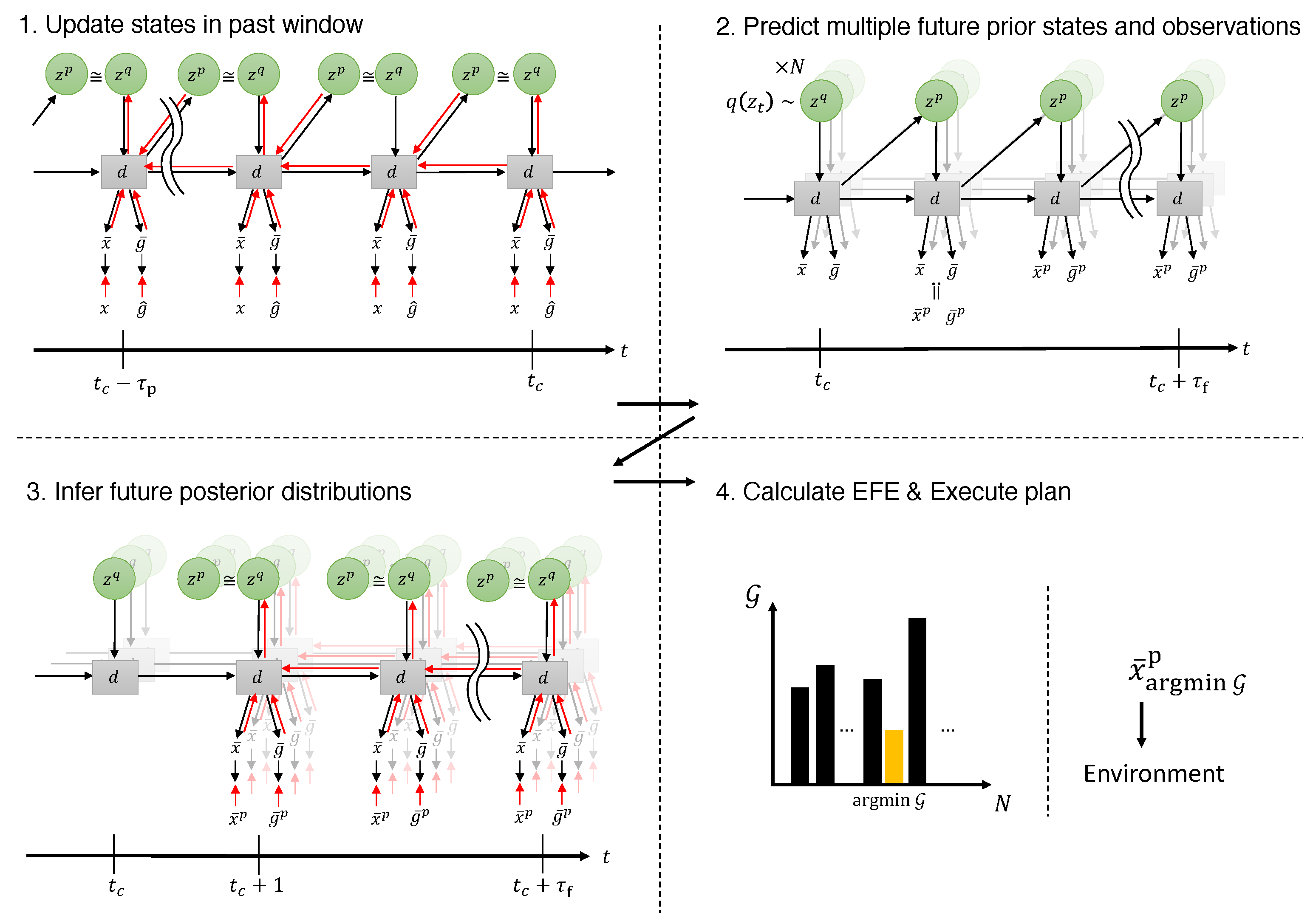
In Experiment 2, we evaluated the proposed model in a continuous action–sensation domain. In this experiment, the agent was placed in a 2D Cartesian space T-maze. Following the original concept image of the T-maze in Experiment 1, a small area at the end of each of the corridors has colored flooring, and the agent possesses a sensor that can determine the color of the floor underneath it. In this environment, we compared our newly proposed model to our previous model, T-GLean, as well as an agent that acts based on habituation by predicting position and color sensation of the next step while minimizing evidence free energy (habituation-only agent). We observed how maximizing information gain is vital for this task and how the prior-preference variance changed over a long sequence of actions for each agent.
In Experiment 3, we examined how the proposed model can modify its action plan to deal with a dynamically changing world. For this purpose, we extended the T-maze environment to include a randomly placed obstacle at the top edge of the maze which could be sensed by the agent using newly added obstacle sensors. We demonstrated how the action plan can be dynamically changed by adapting the approximate posterior in the past window, as well as in the future window, by simultaneously minimizing the evidence free energy and expected free energy. We also tested the robustness of our model by reducing the past observation window, limiting the contribution of evidence free-energy minimization in plan generation.
4.1. Experiment 1
Following the experiment in [
3], we first undertook an experiment in a discrete action space. As shown in
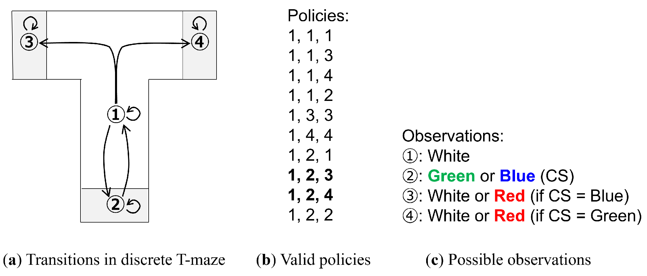
Figure 3a, there are four states that correspond to four possible agent positions in a T-maze: (1) center, (2) bottom, (3) left, and (4) right. This position is encoded as a 4D one-hot vector.
At each of the aforementioned states, a color can be observed. State 1 has a fixed color of white; however, the colors of the remaining states are determined by the color of state 2. State 2 has a 50/50 chance to be either green or blue, and is referred to as the conditioning stimulus (CS). If the CS is blue, then state 3 is red and state 4 is white, and if the CS is green, then the colors of states 3 and 4 are reversed. The observation of the current state is encoded as a 4D one-hot vector of the possible colors: blue, green, red, and white. Note that unlike in [
3], the relationship between the CS and the position of the red color is deterministic.
Along with each state having a self-connection, state 1 has transitions to states 2, 3, and 4, while state 2 has a transition to state 1. States 3 and 4 are terminal states. Using policies of length 3, 10 valid policies are enumerated, as shown in
Figure 3b.
Finally, an additional 2D one-hot vector, indicating whether the position with the red observation has been reached, is provided as an extrinsic goal. Note that [
3] refers to the red color as the unconditioned stimulus (US); however, we refer to it as the goal, following our previous terminology.
The agent always starts at position 1 (center) and has no information on the location of the goal. From an outside observer’s perspective, it is clear that in order to reach the goal reliably, it is desirable to first visit state 2 and check the CS, since it will reveal information on the position of the goal. We note that there are two policies that fit this description (bolded in
Figure 3b), and unlike in our previous work, where the human tutor would provide examples of the preferred behavior, the agent must select the appropriate policy from all possible policies. In this context, a preferred policy is one that first checks the CS and then finds the goal.
To train the PV-RNN, 20 training sequences of length 3 were generated, corresponding to all of the valid policies shown in
Figure 3b, repeated once for the goal being in either state 2 or 3. The dimensionality of each sequence, as described above, was 10. The PV-RNN was trained for 500,000 epochs using the Adam optimizer and a learning rate of 0.001. The trained PV-RNN was then tested over 100 trials, with each trial having
samples. Each trial was conducted with a different random seed. During testing, inference of both the past approximate posterior and future approximate posterior was performed over 100 iterations per time step, with an increased learning rate of 0.1. After sampling, the policy with the lowest EFE (argmin) was selected. We discuss our policy selection methodology in more detail in
Appendix A. In the following results, we examine the agent at the initial time step, after it has observed state 1 and before it moves to the next state.
The results of Experiment 1 are summarized in
Table 2. We observe that the PV-RNN-generated policy samples approximating the training distribution—as noted earlier, only 2 of the 10 possible policies follow the preferred pattern, and only one of them will lead to the goal. However, when selecting the lowest-EFE policy, the preferred policy is selected 100% of the time. Moreover, there is a significant difference in the EFE of policies that match our preferences compared to all other policies. We summarize our analysis of this phenomenon in
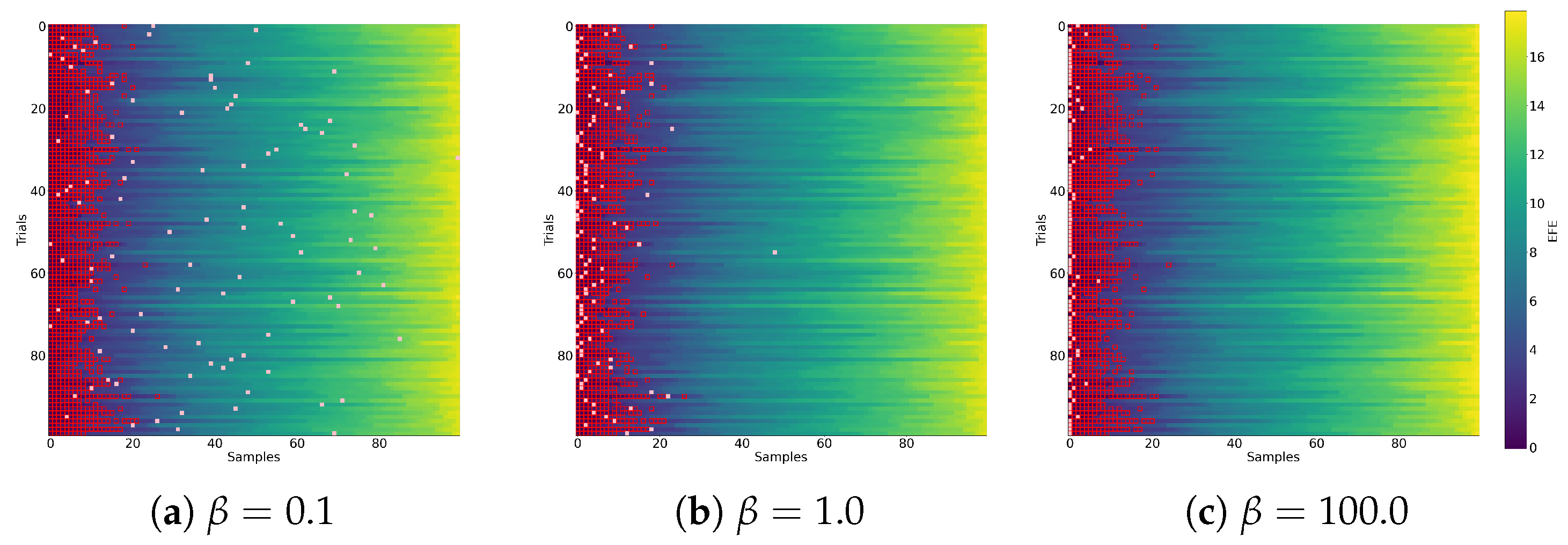
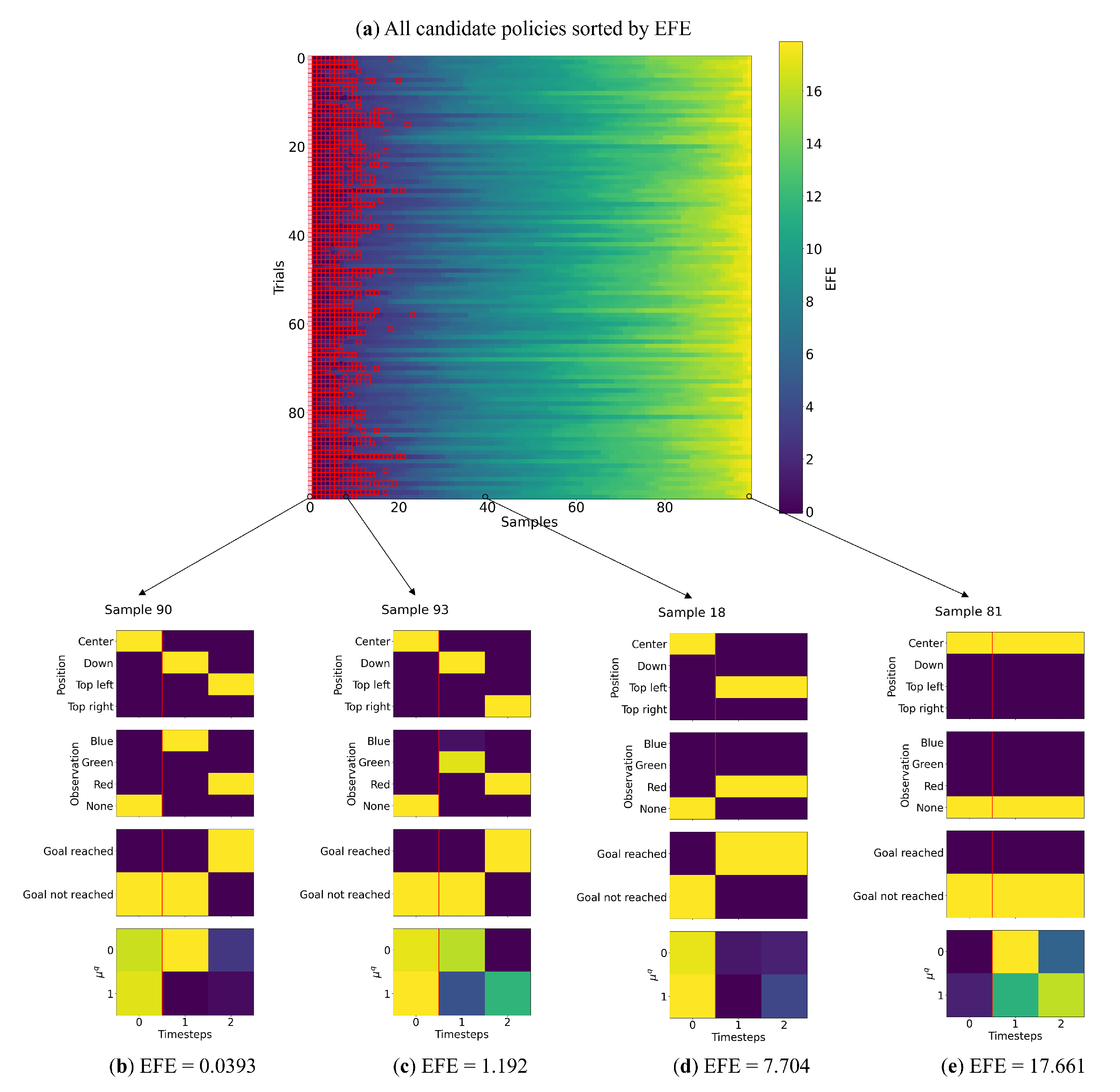
Figure 4.
Figure 4a depicts a graphical representation of the sample selection process when considering all samples. We observed that the preferred policies (highlighted with red boxes) were largely clustered to the left when policies were sorted by lowest EFE.
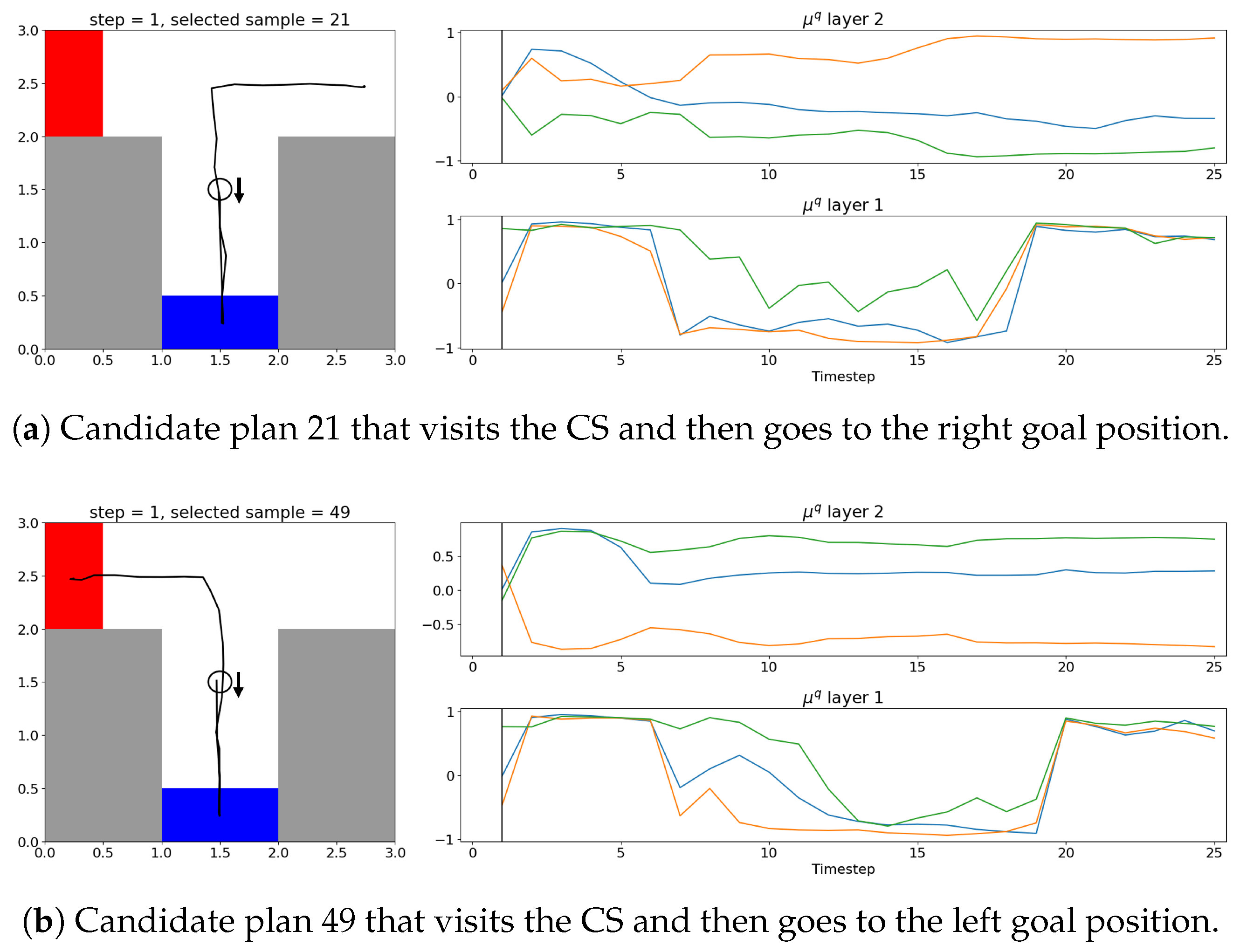
Figure 4b–e break down a single trial, where we observed that the policies with low EFE matched our preferred policies (visiting the CS and then the goal). As the EFE increases, there are policies that have the agent go directly to states 3 or 4, followed by policies that have the agent not move towards the goal at all. From these results we can surmise that the policies likely to be selected, although uncertain about the goal position due to lack of information, will all go to state 2 to maximize information gain.
Observing the latent state activity, there is a difference between policies where the agent visited the CS (
Figure 4b,c) compared to those that did not (
Figure 4d,e). This may indicate actional intention. Additionally, in this setting, it appears that the cutoff for preferred policies occurs at an EFE value of approximately 2.0, with more diverse policies at higher EFE values.
4.2. Experiment 2
Experiment 1 had a limited state space and time horizon; however, our robots operate in a continuous action space and with a much longer time horizon. To simulate this, in this experiment we expanded the discrete T-maze into a 2D T-maze, with the agent position given in 2D Cartesian coordinates. The perception of the agent remained, as in the previous experiment, a 4D one-hot vector encoding the four possible colors. The goal-reached vector was replaced with a goal-sensation vector, a 4D one-hot vector encoding the color of the final sensation, which in this experiment could be red or white. This teleological representation of the goal follows our previous goal-directed planning approach in T-GLean. In addition, to be consistent with our previous work, we use the term plan when describing the generated sequences of actions. We note that while a policy, in the context of active inference, contains only future actions, as our focus is on how to select future action sequences using EFE, we consider the terms plan and policy interchangeable.
As in the discrete T-maze, the agent always starts in the center of the maze, which in this case is at
. From there, it can follow four possible trajectories, with a 50/50 chance of ending at the goal position. The possible trajectories are summarized in
Figure 5. Note that we have removed the cases where the agent remains idle and does not attempt to reach the goal, since as shown in the previous results those plans are very unlikely to be selected by the agent. In this setting, when considered independently, the probability of the agent checking the CS or finding the goal is 0.5.
The agent’s movements were controlled by a simple proportional controller that received and translated it to agent position, while sensor noise was simulated as a Gaussian distribution on the position, with when the agent was in motion and when stationary. The simulation time interval was set at 0.5. To collect training data, the agent followed a series of waypoints to form trajectories traversing the middle of the corridors, with stops in the center of the colored areas at the ends of the corridors. Due to the aforementioned added noise creating some run-to-run variability, each of the possible trajectories was repeated 10 times, for a total of 80 training trajectories. Each trajectory had a length of 25 time steps and a dimensionality of 10. The PV-RNN was trained for 200,000 epochs, with the optimizer settings being identical to Experiment 1.
In this experiment, we examined the behavior of our agent as it moved through the maze, and compared our current EFE-GLean agent to our previous T-GLean and a “habituation-only” agent described previously. As in Experiment 1, each agent undertook 100 trials with random goal placement, and samples.
Table 3 summarizes the results of Experiment 2. We note that the EFE-GLean agent was consistently able to find the goal by first checking the CS, as suggested by the previous experiment, while the two baseline approaches, which did not sample EFE, performed significantly worse. The agent applying VFE minimization (habituation-only) showed a CS rate (chance to check the CS) of approximately that of finding it by chance, which follows the training data distribution. The success rate was higher than in the training data, which suggests that the instances where the agent visited the CS had a higher chance of finding the goal.
Our previously proposed T-GLean, which does not consider information gain, did not move back to check the CS at all, instead it always attempted to go directly to the goal, resulting in a random chance of it succeeding in finding the goal. This result is not unexpected, since T-GLean expects a human tutor to demonstrate the appropriate behavior—in this case, the human tutor would manipulate the agent to go down to check the CS, then go to the correct goal position. However, in this setting where the training data does not bias the agent’s behavior, T-GLean’s lack of intrinsic motivation for self-exploration led it to constantly generate suboptimal action plans.
To investigate this, we compared two cases of selecting the lowest- and highest-EFE plans in
Figure 6 and
Figure 7, respectively.
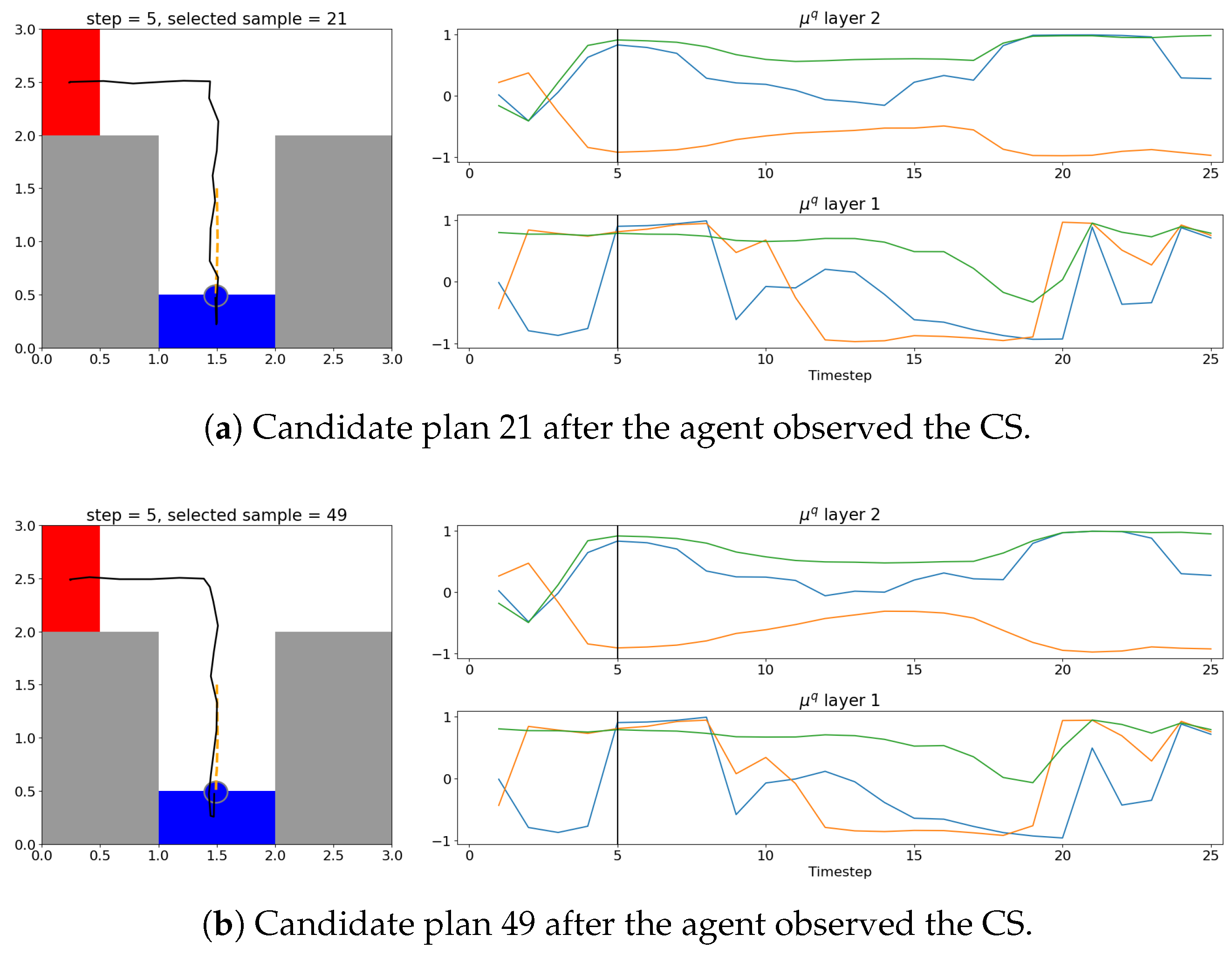
Figure 6 follows the progression of the agent from the start of the trial to the end. A video with several examples from Experiments 2 and 3 is available at
https://youtu.be/I_R2tFh_OxY (accessed on 19 June 2025). The thick black line in the left subplots indicates the selected plan’s trajectory, while the thick black line in the right subplots shows the selected plan’s EFE at each step over the course of the trial. Note that all other candidate plans’ trajectories and EFEs are overlaid in a light gray for reference. At the initial step, where the agent starts with no information, there was a diverse set of candidate plans. The plan with the lowest EFE was selected, which was a plan that moves the agent back to check the CS. During this phase, where the future uncertainty is high (as seen by a diverse set of trajectories the agent could follow), the agent tends to prefer exploratory behavior, as shown by the preference towards plans that move the agent to the CS.
As the agent moves and updates its possible future observations and actions, the ceiling on future information gain naturally declines, corresponding to the decreasing EFE, that reached a minimum as the agent approached the CS. This behavior is in line with the expectation that checking the CS grants the agent all the necessary information to reach the goal, and that further exploration is unnecessary. Once the agent observes the CS, the agent preferentially exhibits exploitative goal-seeking behavior, where all candidate plans are optimized to reach the now-known goal position. We examine the activities of latent variables during the exploration and exploitation periods in a comparative manner in
Appendix B.
Figure 7 shows the plan with the highest EFE, plotted in the same way as
Figure 6a. While this plan takes the shortest path directly to a possible goal, such plans tend to have a high EFE and are not preferred by EFE-GLean.
We note that in both
Figure 6 and
Figure 7, as the trial continues and the agent moves towards the goal, the EFE appears to slowly rise, which could switch the agent back to exploratory behavior. However, this “bored” behavior is not desirable for our goal-directed agent, as this can cause destabilization of the PV-RNN internal states and potentially unsafe movements of the agent.
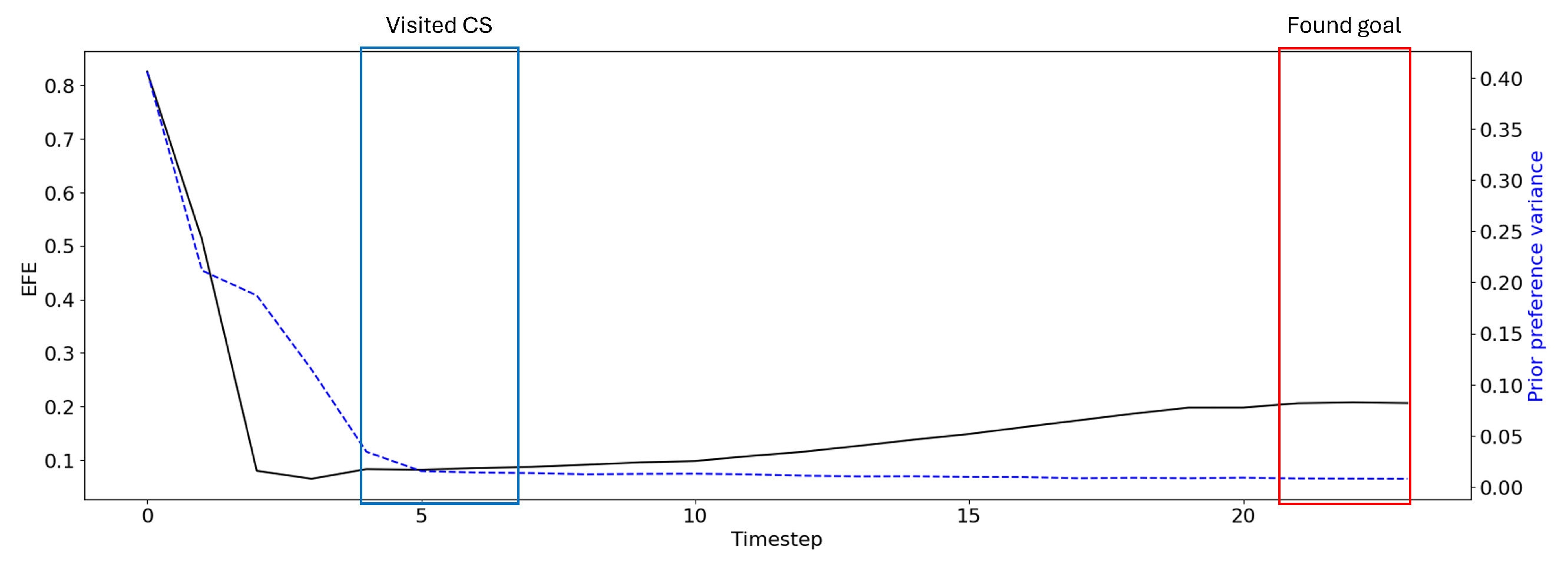
As such, as described in
Section 3, we computed the prior-preference variance in
in order to manage the preference between maximizing epistemic and extrinsic values. To analyze the relationship between prior-preference variance and EFE, we present EFE without prior-preference variance (i.e.,
).
Figure 8 compares the EFE of a given plan without considering prior preference variance to the calculated prior-preference variance. In the condition where the agent is certain of its future, the prior preference is strong and thus the agent prefers to maximize extrinsic value, resulting in stable goal-directed behavior over an extended time horizon.
The results of this experiment in a longer continuous action space demonstrated that our agent was consistently able to exploit information gain maximization until the goal position became certain, at which point stable goal-directed behavior was exhibited with reduction of the prior-preference variance.
Equivalently, when the goal position became certain, there was an increase in the precision of the prior preferences. This is similar to the simulations of dopamine discharges based upon the precision of posteriors over policies explored in prior work [
25]. Here, we are using a simpler setup and the adaptive precision has been specified heuristically (as opposed to being optimized with respect to variational free energy). However, the similarity in the dynamics of the implicit precision is interesting.
4.3. Experiment 3
Our previous study demonstrated that the T-GLean agent can adjust its plan dynamically when the environment changes, and the current study evaluated this capability of EFE-GLean. This was accomplished through optimization of the adaptive vector (
), as demonstrated in
Appendix C. Experiment 3 tested whether the EFE-GLean agent could prepare action plans in an extended T-maze task when anticipating an obstacle hidden in the environment, and could update the plans adequately when the obstacle was actually sensed.
Following on from Experiment 2, the T-maze environment was extended by adding a randomly placed obstacle along the top wall, outside of the goal areas. The obstacle blocked half of the corridor, requiring the agent to take a detour to avoid collision. In order to detect the obstacle, the agent was equipped with four range sensors placed at 45 degrees to the cardinal directions. These four sensors return a floating point value between 0.0 and 0.7, sufficient to sense its immediate surroundings (the corridor width is 1.0). The obstacle is always outside of the range of the sensors at the initial position of the agent. In addition, the color representation was changed from a one-hot vector to a more realistic RGB representation, with each channel being a floating point value between 0.0 and 1.0. The colors in the environment remained unchanged. The agent position remained represented by a Cartesian coordinate; however, the simulator time interval was reduced to 0.2. In this way, the agent was given additional time steps to sense the obstacle, slow down, and maneuver around it if necessary.
The training data was collected in a similar fashion to Experiment 2, except now with each of the eight possible patterns shown in
Figure 5—four training sequences had a randomly placed obstacle along the top edge of the maze and another four sequences had no obstacle—for a total of 64 training sequences. While collecting data, the agent attempts to remain centered in the corridor by maintaining an equal distance based on observations from its range sensors, and slows down when taking the narrow path next to the obstacle. The total number of time steps was extended to 60, with each sequence having a dimensionality of 12. The PV-RNN was otherwise configured and trained as in Experiment 2.
To analyze the robustness of EFE-GLean, we conducted an ablation study where we reduced the past window
, which reduces the evidence free energy, as given in Equation (
6). The results are summarized in
Table 4. When we reduced
to half length (30 steps), we observed that while the exploration behavior remained intact, the goal-directed behavior became degraded, as the agent appeared to forget the CS in some cases and select a plan to go to the incorrect goal position.
Put simply, the minimization of variational free energy provides posterior beliefs about the current states of the world. These beliefs are then used to evaluate the expected free energy using posterior predictive densities in the future. This means if the agent is uncertain about the current state of affairs—due to a reduction in —it will also be uncertain about the future and the consequences of the different policies it could pursue.
In the extreme case where was limited to a single step, the success rate degraded to below the training baseline, largely due to the agent being no longer able to adequately navigate around obstacles.
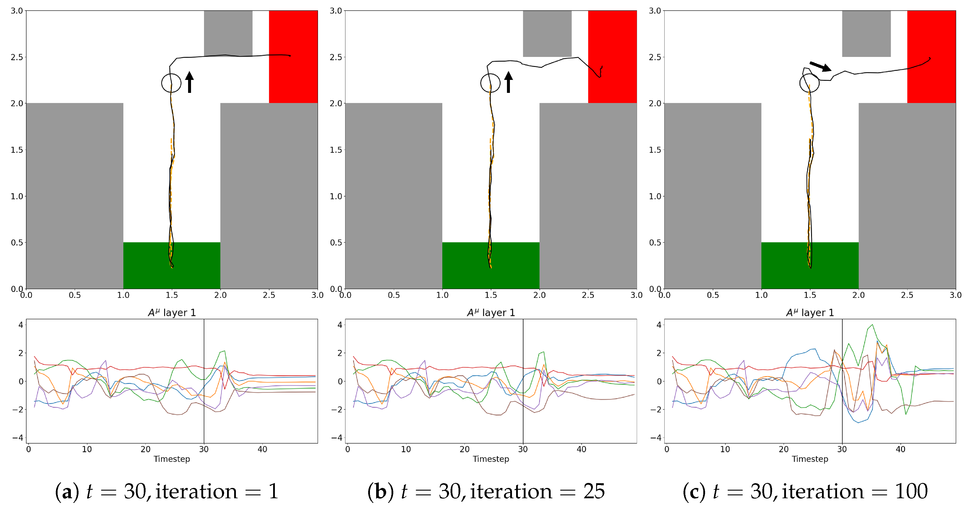
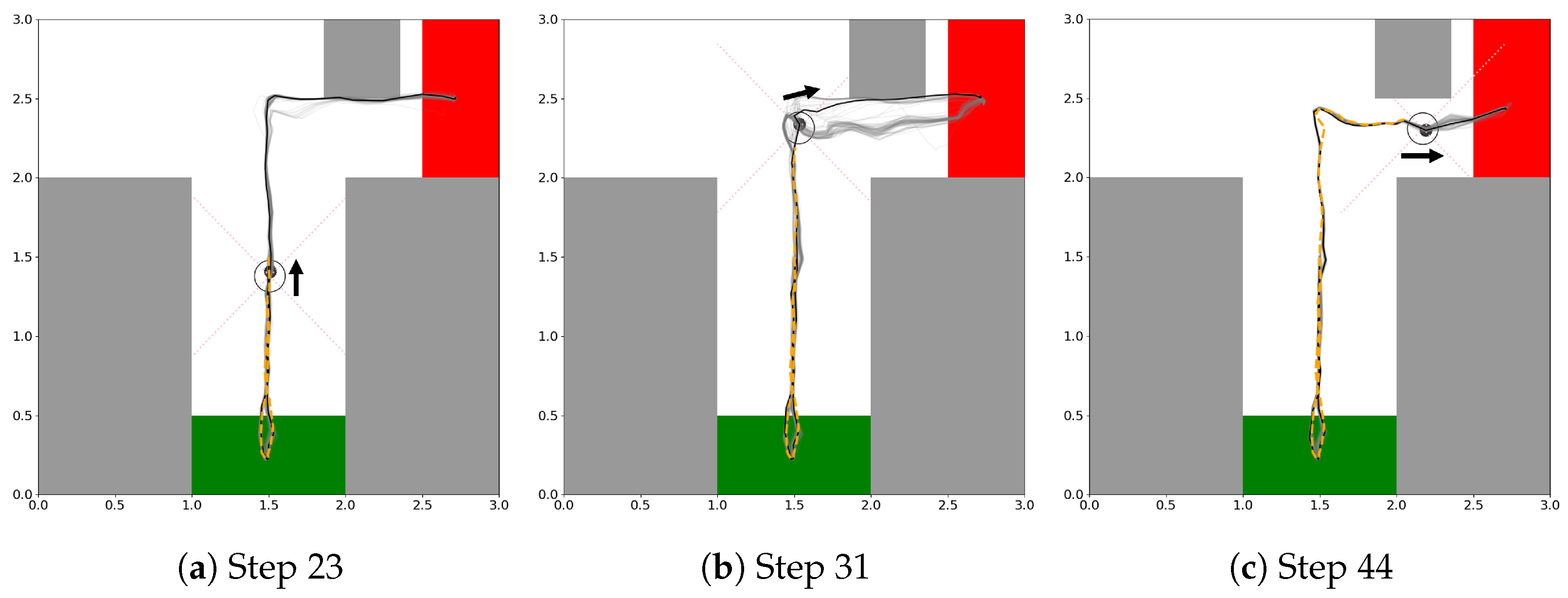
In the analysis of the plan trajectories dynamically generated during travels of the original EFE-GLean agent, some interesting behavioral properties were observed (a typical example is shown in
Figure 9). In
Figure 9a, after checking the CS, the agent generated the shortest path going toward the goal which could collide with the obstacle since it had not yet been detected. However, there was some uncertainty in the trajectories due to the possibility of the obstacle being located at various positions. In
Figure 9b, immediately after detecting the obstacle, two plan options, one for taking the shortest path to the goal and the other for detouring around the obstacle, were generated before the convergence of the plan. Finally, in
Figure 9c, the plan converged to the one that stably arrives at the goal by detouring around the obstacle.
These experimental results demonstrate that EFE-GLean retains the ability to rapidly adjust its plan independently of its exploration behavior. As shown in our previous work, this is an important ability when operating robots in the physical world with the potential for sudden environmental changes.
