1. Introduction
Oil-immersed transformers are a critical component of power systems, being responsible for voltage transformation and power transmission. When faults such as overheating or discharge occur, if not promptly identified and handled, they can disrupt the stability of the power system and severely threaten the safety of the power grid [
1,
2]. Among the transformer fault diagnosis methods, the Dissolved Gas Analysis (DGA) technique has developed rapidly and achieved significant results. DGA assesses the transformer’s operational status and potential fault types by monitoring the composition and concentration changes of dissolved gases in the transformer oil. Typically, the dissolved gas content in transformer oil is stable; however, due to insulation aging, electrical faults, or thermal faults, specific gases such as H
2, CH
4, C
2H
6, C
2H
4, and C
2H
2 are produced. The composition and concentration changes of these gases can effectively reflect the type and severity of faults [
3,
4].
The three-ratio method is widely used in transformer DGA due to its clear principles, well-defined standards, and simplicity of operation [
5]. It involves calculating three specific gas ratios which correspond to different types of transformer faults: CH
4/H
2, C
2H
6/CH
4, and C
2H
4/C
2H
6. These ratios are then compared with diagnostic charts or the threshold values specified in the IEC 60599 standard [
6] to identify faults such as partial discharges, overheating, arcing, and so on. Through analyzing these gas ratios, the method enables reliable fault classification without requiring complex computations or specialized equipment. It is suitable for preliminary fault screening and routine monitoring in power systems [
7]. Reference [
8] showed that the three-ratio method can effectively diagnose transformer faults. Reference [
9] improved the three-ratio method by combining it with a BP neural network, successfully constructing a transformer fault classification model. Reference [
10] extended the application of the three-ratio method using spatial interpolation technology, overcoming its limitations through the application of the Belief Propagation Algorithm (BPA). However, the three-ratio method faces issues such as missing encoding, fuzzy critical values, and gas cross-interference. It is also significantly affected by oil sample aging, environmental interference, and mixed fault gases, which limit its ability to recognize composite faults and early potential defects. Furthermore, the use of a static threshold setting makes it unable to adapt to dynamic operating conditions, leading to poor compatibility with low-concentration gases and new insulating oils, thus limiting its application and reliability in complex scenarios.
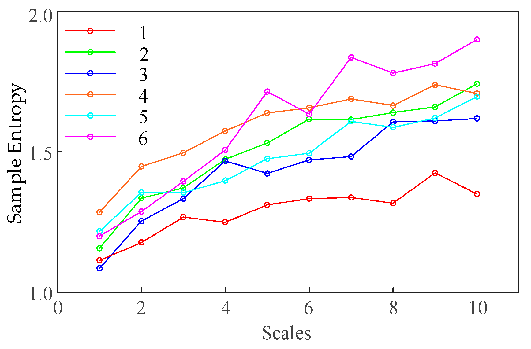
To overcome the limitations of the three-ratio method, this study introduces sample entropy (SE) as a feature indicator for transformer fault diagnosis. Multiscale sample entropy (MSE) allows system complexity to be analyzed at different scales in order to provide a comprehensive understanding of signal behavior, thereby improving the sensitivity of fault detection. Higher SE values typically indicate greater system complexity and uncertainty, which may suggest potential faults. Multiscale entropy has been widely applied in various fields, such as biomedical applications [
11], mechanical fault detection [
12], environmental monitoring [
13], financial market analysis [
14], speech signal processing [
15], image processing [
16], and bio-signal analysis [
17], and has enhanced early fault prediction capabilities in DGA diagnostics. In recent years, deep learning methods have made significant progress in transformer fault diagnosis due to their powerful feature extraction and nonlinear fitting capabilities [
18]. Through constructing deep neural networks, fault features from DGA data can be effectively mined, overcoming the reliance on expert knowledge inherent in traditional methods. Reference [
19] proposed an early fault diagnosis method for electro-hydraulic control systems based on residual analysis. The method extracts residual signal features and optimizes the Bayesian network to correct the fault diagnosis results. Reference [
20] introduced a concurrent fault diagnosis method for electro-hydraulic control systems based on Bayesian networks and D-S evidence theory. They divided the fault diagnosis approach into multiple sub-models, used OOBNs to establish an initial diagnostic model, and then applied D-S evidence theory for information fusion, improving the reliability of the diagnosis. Reference [
21] proposed a ReLU-DBN-based model using unencoded ratios as feature parameters, combined with support vector machines and backpropagation neural networks, thus achieving higher classification performance. Reference [
22] proposed a short-term load forecasting method based on LSTM, which improved the transformer load prediction performance by incorporating historical load, holidays, and weather data, providing technical support for solving overload issues.
Despite the significant achievements of deep learning models in transformer DGA diagnostics, their large number of parameters can consume considerable memory and computational resources, affecting their real-time performance. DGA data are provided in one-dimensional form, and converting them into two-dimensional images presents challenges, with traditional conversion methods having limited effectiveness. Recursive plots (RPs) can transform one-dimensional data into two-dimensional images, but conventional convolution operations struggle to extract features effectively. To address this issue, the Convolutional Block Attention Module (CBAM) is introduced, which optimizes feature extraction by incorporating attention mechanisms along both the channel and spatial dimensions, thereby improving fault diagnosis performance and model efficiency.
Knowledge Distillation (KD) is a technique that transfers knowledge from a teacher model to a student model, effectively compressing the model while maintaining high performance [
23]. Compared with traditional compression methods, KD offers the advantage of balancing lightweight design with performance, compatibility across architectures, and improved training efficiency; thus, KD provides an optimized path for resource-constrained scenarios such as edge computing and real-time inference. Reference [
24] proposes an incremental partial discharge recognition method that combines KD and a graph neural network (GNN). This approach utilizes KD during the incremental training process to prevent model forgetting, while the GNN addresses the issues of small sample sizes and class imbalance, thereby improving the learning performance on new data. Reference [
25] introduced a context-aware KD network, which eliminated the gap between the teacher and student networks using an adaptive channel attention mechanism, improving object detection performance and providing an innovative solution for KD applications in object detection. KD not only applies independently for model compression, but also synergizes with deep learning architectures. The Residual Network (ResNet) introduced the residual block structure, successfully addressing the gradient vanishing problem in deep networks and providing a stable foundation for training complex teacher models [
26]. Deep learning methods combine feature extraction and fault diagnosis in an end-to-end manner, overcoming the limitations of traditional machine learning methods [
27]. Since convolutional layers in deep learning models have weight sharing and local connection properties, they can effectively extract features when processing two-dimensional image data, yielding excellent results. Combining deep learning with KD, using two-dimensional image data for fault diagnosis has become a popular research direction for rapidly identifying potential fault patterns and improving prediction performance.
In summary, the traditional three-ratio method has limitations such as rigid encoding rules, high threshold sensitivity, and insufficient anti-interference ability, which severely restrict its applicability under complex operating conditions. In contrast, although deep learning-based improved methods have significant advantages in terms of feature extraction, they face the dual bottlenecks of high model complexity and limited data representation capability. These limitations highlight the necessity of developing a feature extraction mechanism with high robustness and a lightweight diagnostic architecture.
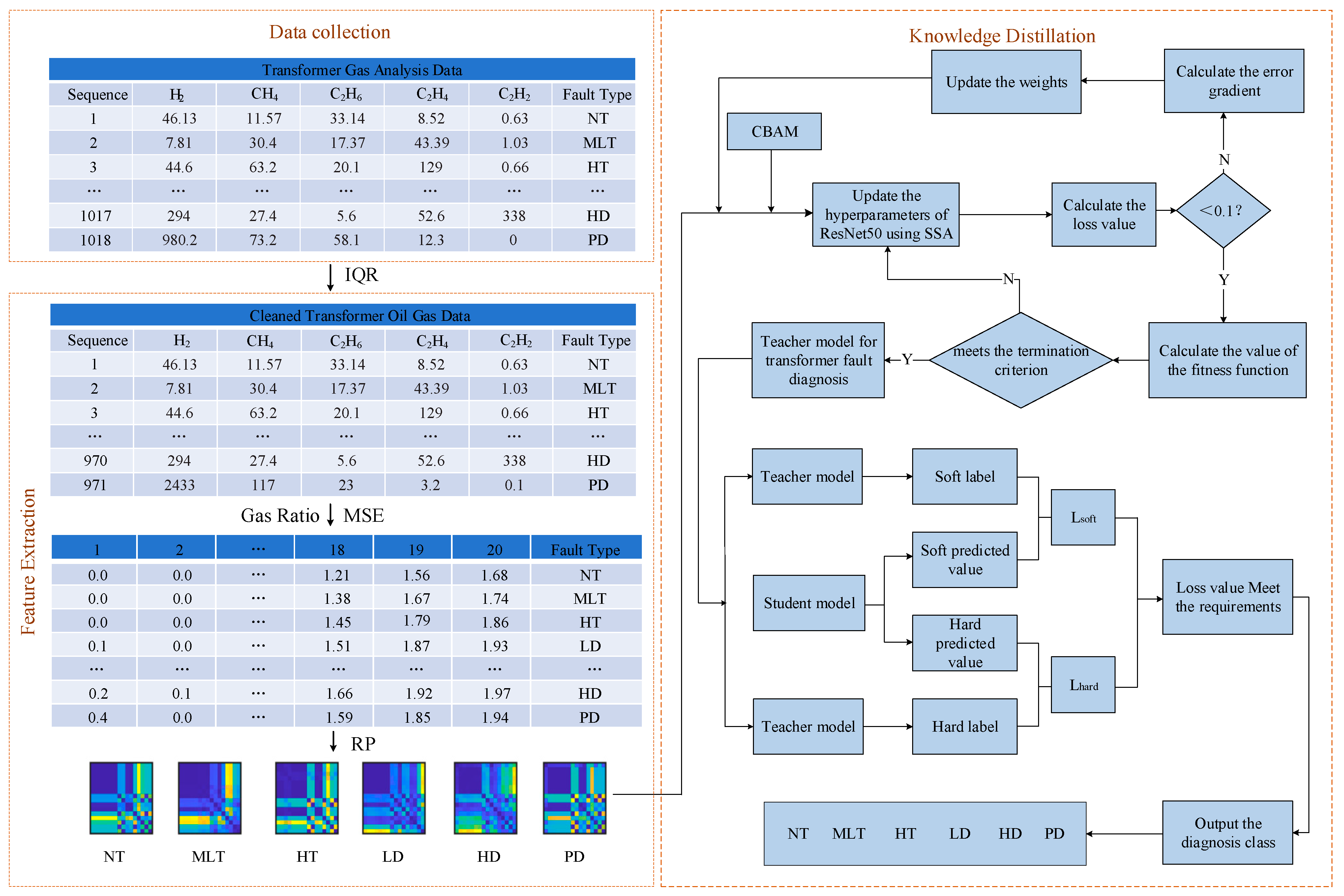
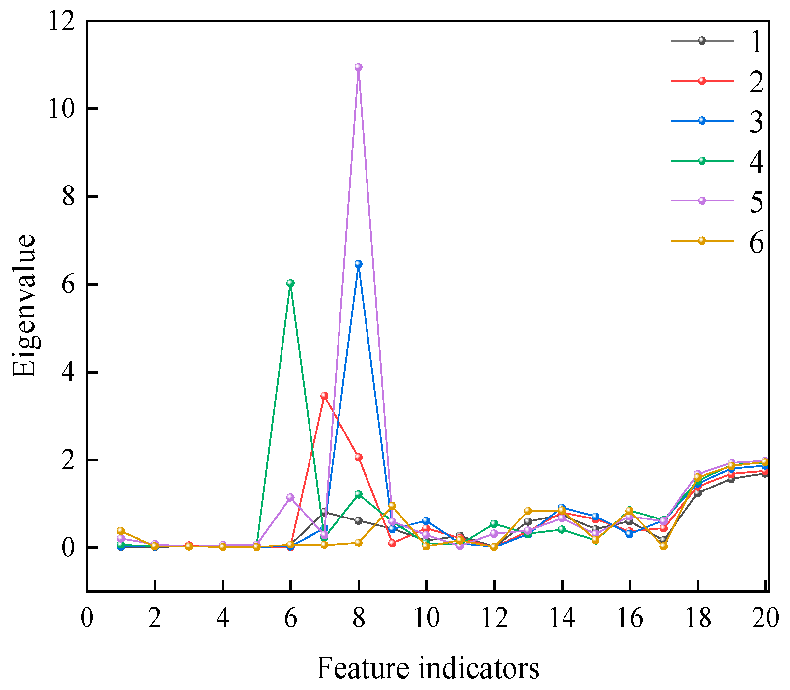
This study proposes a lightweight model using MSE and KD. First, to address the limitations of traditional three-ratio methods and deep learning approaches in feature extraction and computational efficiency, a feature extraction method based on MSE and RP is introduced, effectively improving the sensitivity and accuracy of transformer fault detection. Secondly, the CBAM is introduced to optimize the feature extraction process of ResNet50, enhancing the model’s ability to focus on key features. Finally, by combining KD technology, a lightweight model is designed that reduces computational resource consumption while maintaining efficient DGA diagnostic performance. The experimental results demonstrate that the proposed model excels in terms of diagnostic accuracy, computational complexity, and storage requirements, providing an efficient and reliable transformer DGA diagnostic solution.
The remainder of this article is structured as follows:
Section 2 introduces the principles of the relevant algorithms.
Section 3 presents the model based on MSE and KD-CNNs.
Section 4 demonstrates the performance of the proposed diagnostic model.
Section 5 concludes the study.
2. Algorithms and Principles
This chapter introduces the key algorithms and principles underlying the construction of a transformer DGA diagnostic model. Based on transformer DGA data, various algorithms are applied to extract effective features, enabling efficient fault diagnosis. First, the chapter introduces the fault mechanisms and distribution of transformers, followed by an explanation of how MSE improves DGA diagnostic accuracy by analyzing the complexity of data at different time scales. Next, leveraging the features extracted through MSE, the integration of KD and CNN models is discussed. Through KD, the teacher model transfers effective knowledge to the student model, reducing computational load and optimizing model performance. Furthermore, the introduction of RP and CBAM further enhances the feature extraction process. RPs effectively convert one-dimensional data into two-dimensional image features, improving model interpretability, while CBAM uses both spatial and channel attention mechanisms to enable the model to focus on key regions during feature learning.
2.1. Transformer Fault Mechanisms and Distribution
Transformer faults result mainly from irreversible damage to insulation materials and conductive components due to thermal stress and electrical discharges. Thermal faults, accounting for 55–60%, are primarily caused by overheating due to issues such as loose connections, core eddy current losses, or winding defects. Electrical faults, making up 35–40%, are triggered by insulation aging, moisture, or mechanical damage.
Faults evolve in stages based on temperature thresholds and gas release characteristics. Thermal faults initially cause local overheating, decomposing oil and cellulose, and thus producing gases such as CH4 and C2H6. As the temperature increases, pyrolysis accelerates, leading to higher concentrations of C2H4 and H2. At critical temperatures, severe overheating generates large amounts of C2H4 and C2H2, degrading the insulation. Electrical faults begin with partial discharge, producing H2 and CH4, and progress to low-energy discharges that release C2H2 and H2. If untreated, high-energy discharges occur, decomposing oil and insulation rapidly, producing gases such as C2H2, H2, CO, and CO2, resulting in catastrophic failure.
Unresolved transformer faults pose significant risks. They disrupt operational stability by interfering with voltage regulation, and high-energy discharges can trigger cascading power outages. Faults also pose safety hazards, such as oil leaks, explosions, and fires, which threaten the safety of personnel and infrastructure. Economically, forced shutdowns and replacements may cost millions of dollars, with direct losses exceeding one million dollars for a single large transformer failure. Environmentally, leaked transformer oil can pollute soil and water, and degradation products of insulation materials may violate environmental regulations.
2.2. Multiscale Sample Entropy
SE is a widely used tool for measuring the complexity of time series, reflecting the system’s dynamic characteristics by analyzing the self-similarity of the data. However, traditional SE methods typically assess data complexity at a single scale, which may not fully capture the multi-level dependencies present in the data. To address this, this study introduces MSE, aiming to provide a more comprehensive analysis of the time series complexity by examining multiple time scales. By considering the complexity at different scales simultaneously, the MSE method effectively captures both short-term and long-term dependencies, thereby enhancing the overall ability to recognize system behaviors.
2.2.1. Sample Entropy
The core idea behind SE is to measure the complexity of a time series by examining the similarity between adjacent samples. The method involves reconstructing the time series into high-dimensional vectors and evaluating the similarity between these vectors to assess the disorder of the series. SE overcomes its limitations by providing more stable results, particularly for short datasets and noisy signals, making it a robust tool for practical applications.
2.2.2. Algorithm Steps
Given a time series , where N is the length of the series, the calculation of SE involves the following steps.
First, the time series
x is reconstructed into multiple vectors of dimension
m, where each vector consists of
m data points. Specifically, each vector is represented as follows:
where
xi represents the data points in the time series,
m is the number of data points in each vector, and
N represents the total number of data points in the time series.
For any two vectors
Xi and
Xj, their similarity is measured by the maximum absolute difference between the corresponding elements. If the maximum difference between the two vectors is less than a predefined threshold
r, the vectors are considered similar. This threshold is usually defined as a multiple of the standard deviation of the time series data.
where
r is the threshold value for similarity,
α is a constant, typically set to 0.1, and
std(
x) is the standard deviation of the time series data
x.
Next, the number of matches is calculated for each pair of vectors Xi and Xj. A match is defined as a pair of vectors whose maximum absolute difference is less than the threshold r.
After obtaining the match counts, the SE is calculated using the following formula:
where
Am(
r) is the proportion of vector pairs that are similar when the embedding dimension is
m, and
Bm+1(
r) is the proportion of vector pairs that are similar when the embedding dimension is
m + 1.
SE reflects the complexity of the time series by comparing vector similarities at two different dimensions. When the time series exhibits simple structures, the number of similar vector pairs is large, resulting in a small SE value; in contrast, when the time series is more complex, the number of similar vector pairs is small, leading to a higher SE value.
2.2.3. Multiscale Sample Entropy Algorithm Steps
MSE is an extension of the traditional SE that is used to analyze the complexity of time series data across multiple temporal scales. While SE measures the complexity of a time series at a single scale, MSE decomposes the original time series into multiple scales, capturing both short-term and long-term dependencies. This multiscale approach provides a more comprehensive measure of the data’s complexity.
The original time series is first decomposed into multiple time series at different scales by downsampling the data. For each scale
, downsampling is performed by averaging the data within non-overlapping windows of size
. The downsampled time series at scale
is calculated as follows:
where
is the scale factor, and
represents the data points in the original time series. The new time series
is the average of the data points within each window of size
.
Once the time series is decomposed into multiple scales, the traditional SE is calculated for each scale. SE is computed by reconstructing the time series into vectors and measuring the similarity between these vectors. The calculation of SE for each scale follows the same procedure as in the original SE method.
The formula for SE at scale
is given by
where
and
represent the proportions of similar vector pairs at dimensions
m and
m + 1, respectively, for the time series at scale
, with a predefined similarity threshold
.
Finally, the SE values calculated at each scale are averaged to obtain the MSE.
where
S is the number of scales, and
is the SE calculated at scale
τ.
2.3. Knowledge Distillation
KD is essentially an efficient knowledge transfer method that minimizes the model size by extracting and transferring knowledge from a teacher model to a lightweight student model. Typically, the output of neural networks uses hard labels marked with 0 s and 1 s, which ignore the information from other related classes except the correct one; in contrast, soft labels have values between 0 and 1, which not only indicate the class attribute but also encapsulate implicit information about the relationships between different classes. The teacher model extracts features from labeled training samples and generates high-quality soft labels. These soft labels contain not only the class information of the samples but also reflect the similarity between classes, providing the student model with rich supervisory signals. During the learning process, the student model enhances its prediction ability by mimicking the outputs of the teacher model. This method allows the student model to achieve performance close to or matching that of the teacher model while maintaining a lower complexity.
KD mainly involves the following two key steps.
- (1)
Soft label generation and distillation temperature. The output of the teacher model is not only the standard hard labels, but can also be smoothed by a temperature coefficient β to generate soft labels. The smoothness of the model output is controlled by adjusting β. A higher temperature coefficient results in a smoother probability distribution, which provides relational information between classes, allowing the student model to learn more latent feature information, rather than just the classification performance.
- (2)
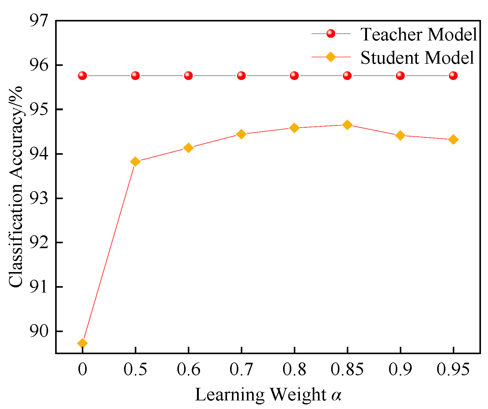
Combination of soft labels and hard labels. The training of the student model involves learning not only from the soft labels generated by the teacher model, but also from the real hard labels. To balance the influence of the soft and hard labels during training, a weighting coefficient α is introduced to combine their contributions. The loss function is calculated as follows:
where
LKD is the total loss function of the student model,
Lhard is the loss associated with the hard labels,
Lsoft is the loss associated with the soft labels, and
α is the coefficient that controls the relative importance of the hard and soft labels. By adjusting the value of
α, one can control whether the student model focuses more on the hard or soft labels during training.
Since ResNet50 employs a residual block structure, it addresses issues such as vanishing gradients that are common in deep networks. This enables it to effectively extract complex features from the data and generate high-quality soft labels. Therefore, ResNet50 is chosen as the teacher model in this study.
MobileNet, as a network model designed for resource-constrained environments such as mobile devices and embedded systems, utilizes techniques such as depthwise separable convolution and dilated convolution. These techniques improve computational efficiency while reducing the model’s parameter count and computational overhead [
28]. Therefore, MobileNet is chosen as the student model in this study.
2.4. Convolutional Neural Networks (CNNs)
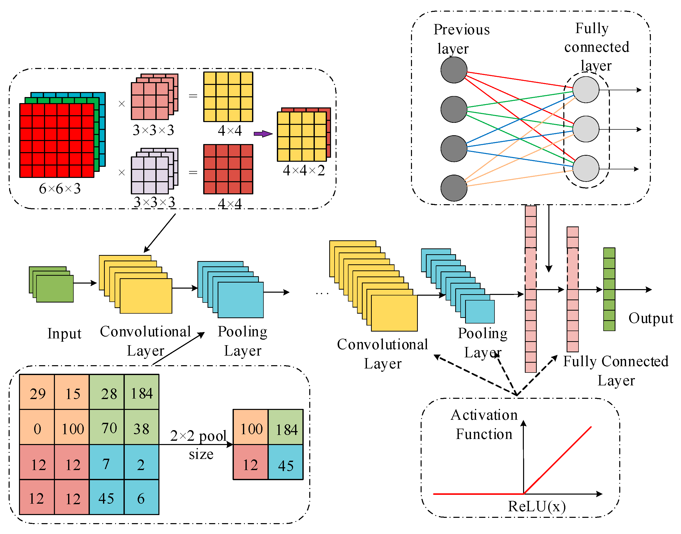
CNNs are a type of deep learning network that include convolutional operations and have a deep layered structure in a feedforward manner. The structure of a CNN mainly consists of convolutional layers, pooling layers, activation layers, and fully connected layers. The convolutional layer extracts local features from the input data through convolution operations, the pooling layer performs dimensionality reduction on the features, the activation layer introduces nonlinear transformations, and the fully connected layer is used for the final classification or regression task. The specific structure is shown in
Figure 1.
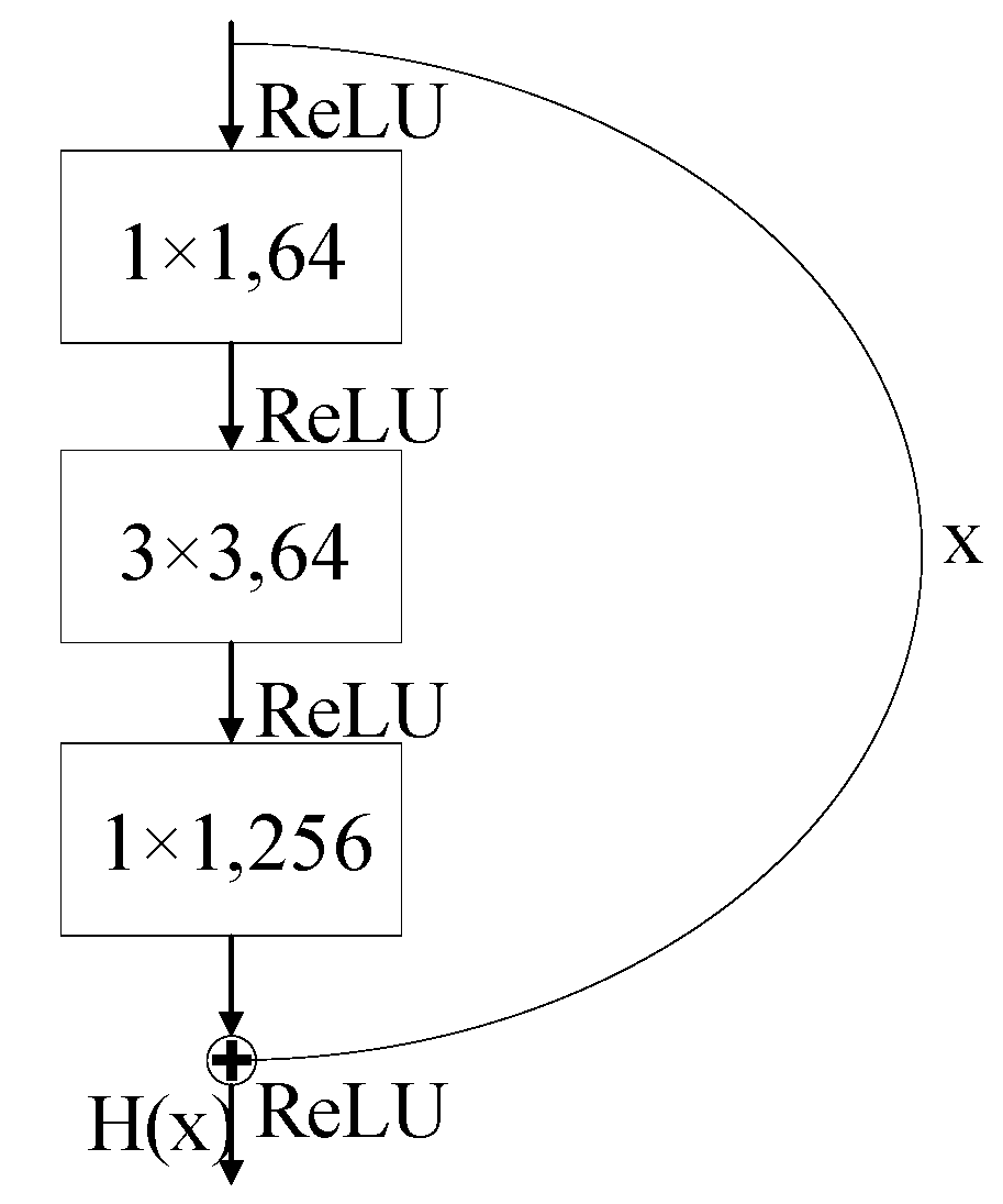
ResNet50 and MobileNet are two popular CNN models. ResNet50 is a deep residual neural network that effectively alleviates the vanishing gradient problem in deep networks through the design of skip connections in its residual blocks. The core residual block in ResNet50 consists of three convolutional layers that form a bottleneck structure, and residual learning is achieved by adding the input features to the output [
29]. The network progressively reduces the feature map size through convolutions at different stages, while simultaneously increasing the number of channels, enabling multiscale feature extraction. When the input and output dimensions do not match, shortcut connections adjust the dimensions using 1 × 1 convolutions, ensuring the integrity of the network structure. The structure is shown in
Figure 2.
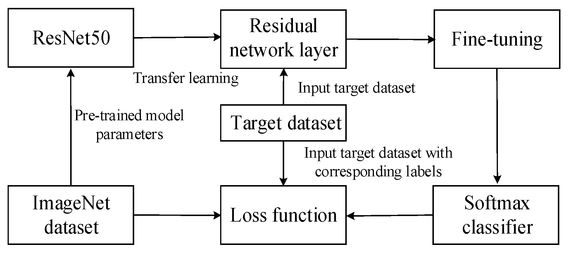
ResNet50, with its powerful feature extraction capabilities, effectively handles high-dimensional and large-scale fault data, identifying complex fault features from them. By introducing residual blocks, gradient propagation through the network is facilitated, thereby accelerating the model’s convergence speed and enhancing the reliability of fault diagnosis. ResNet50 has demonstrated robust performance and strong generalization ability in tasks such as image classification, object detection, and image segmentation, making it a valuable tool in image processing. The specific implementation is shown in
Figure 3.
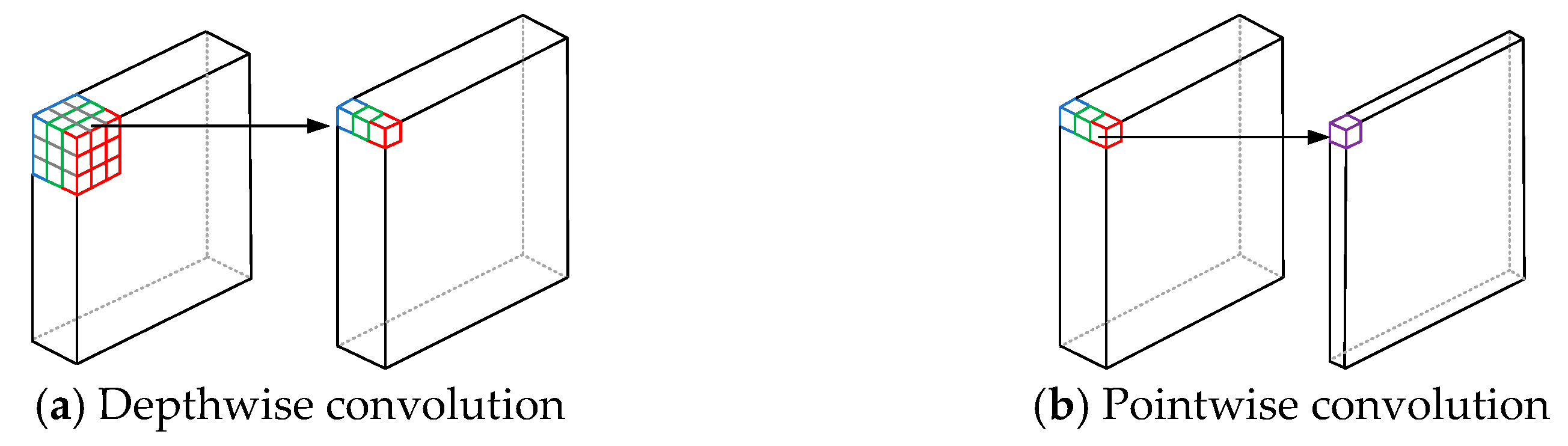
MobileNet is a lightweight convolutional neural network designed specifically to run on resource-constrained devices. Its core innovation is depthwise separable convolution, which decomposes the traditional convolution operation into two steps: depthwise convolution and pointwise convolution. This greatly reduces computational complexity and the number of parameters. Although MobileNet has a relatively simple structure, it still performs well and is suitable for scenarios with low computational resource requirements. The depthwise separable convolution module is shown in
Figure 4.
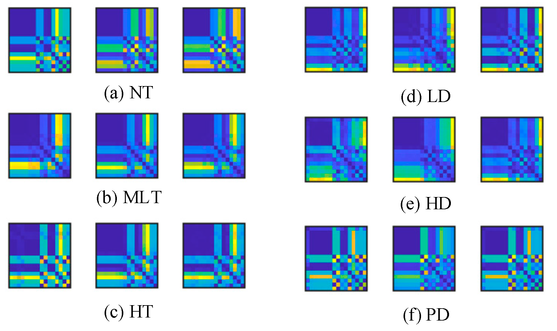
2.5. Recursive Plot
RP is a visualization tool used for analyzing data patterns, designed to visually represent the similarity between data points [
30]. In an RP, each data point is mapped to a node in the plot, and the connections between nodes indicate the similarity or dependency between them. The advantage of the RP lies in its ability to capture latent patterns and relationships in the data through the plot’s topological structure without assuming any specific structure for the data. The RP structure is constructed by calculating the similarity between data points, as shown in the process described in Equation (8).
In the equation, R(i, j) represents the similarity between data points xi and xj, and ϵ is the predefined threshold. The Euclidean distance is used to measure the similarity between data points. When the distance between two points is smaller than the threshold, a connection is established between them; otherwise, no connection is formed.
2.6. Convolutional Block Attention Module (CBAM)
CBAM includes the channel attention and spatial attention modules [
31]. The implementation of channel attention is shown in Equation (9):
In the equation, X represents the input feature map, GlobalPooling denotes the global pooling operation, FC is the fully connected layer, and σ is the Sigmoid function used to generate the weight Mc.
The implementation of spatial attention is shown in Equation (10):
In the equation, MaxPooling and AvgPooling represent the max pooling and average pooling operations, respectively. Conv2D is the convolution operation, and the spatial attention map is generated through σ.


