1. Introduction
Neural networks (NNs) that mimic animal NN behavior are an algorithm to process distributed parallel information. Because of the complexity of NNs, the relationships between internal nodes are adjusted to deal with information in network. Regardless of the type of NNs, they have some common characteristics, such as massively parallel processing, distributed storage, and topology elasticity [
1,
2].
In contrast to pure Markov processes, only the transition time and probability of semi-Markov processes are determined by the time required for the system to reach its present state. Markov theory is named after Russian mathematician Andrei Markov, who pioneered the systematic study of how stochastic processes can be described mathematically. Semi-Markov processes were proposed by Paul Levy in 1954 to build more general models for probabilistic systems. This class of models are used to analyze complex dynamic systems and are often used in reliability calculation. For semi-Markov jump NNs, extended dissipativity was considered by considering partly unknown transition rates [
3] or known transition rates [
4], and state estimation [
5,
6] problem are studied by applying different methods, respectively.
Finite-time control [
7], due to its characteristic, has been widely applied in various fields. Usually, the system state is required to run within a limited time interval and has good performance indicators within a given time [
8,
9,
10]. For finite-time Markov problems in NNs, the
boundedness [
11] was analyzed, synchronization [
12] was shown, and
–
state estimation [
13] based on unreliable communication links was obtained, respectively. For semi-Markov NN problems, finite-time synchronization control [
14,
15] was studied, and the
–
synchronization [
16] was analyzed, respectively.
Because faults in modern industrial systems are inevitable, faults also happen in NNs. Faults happening may cause serious results. To deal with this problem, fault-tolerant control (FTC) [
17] was proposed. The FTC problem [
18] in NNs was studied based on ADP methods. The extended FE observer [
19] was designed to propose an FTC method for discrete Markovian jump systems. A control protocol with actuator fail-resistant performance was adopted to ensure reliable leader–follower consensus [
20]. To save more network resources, a new event-triggering method was proposed which was not constrained by actual system state and designed a reliable observer-based controller [
21].
In particular, results [
22,
23] on semi-Markov NNs existed. Based on the semi-Markov jump model with actuator faults as random variables [
22] in NNs, the criterion of passivity FTSC was analyzed. The improved mean-square exponential stability criterion [
23] was derived, and then an FTC strategy was proposed by using several decoupling techniques.
Since faults were not considered in [
14,
15], which motivates our discussion, we discuss a finite-time
-dissipative FE and event-triggered FTSC for semi-Markov NNs. The highlights of this paper are listed:
- (1)
The error system between master system and slave system are obtained, and then an intermediate FE method is designed so that the state, fault, and intermediate variables are estimated, which provides information for FTSC protocol proposed. The intermediate observer can obtain better fault estimation results than the general observer [
19].
- (2)
Considering the event-triggered condition designed and estimate information, an FTSC protocol is presented to analyze stochastic FTSC with
-dissipativity of error systems with finite time. This finite-time scheme can converge quickly and achieve FTSC more quickly than asymptotic stability schemes [
19].
- (3)
The proposed scheme not only estimates faults, but also proposes the FTSC protocol, which belongs to the active FTC category and is more suitable for practical engineering field.
2. Problem Statement
A NN as master system is that
in which
denotes state of neuron’s state;
is measured output;
denotes neuron activation function;
denotes time-varying delay satisfied
and
,
are given; diagonal matrix
; and matrix
,
,
are known. For
,
is a discrete-time state semi-Markov process with values in
with
, where
if
,
if
, and
,
is transition rate from mode
i at
k to mode
j at
and
. For simplicity, set
, then
,
,
,
; the other symbols are similar expression.
A corresponding NN as slave system is that
in which
,
, and
are similar definitions in master systems, and
denotes the control input.
denotes external disturbance and
denotes the fault, which are different and
is bounded.
,
, and
are known matrices.
Define
,
, then error system between NN (
1) and (2) and NN (
3) and (4) is
where
Assumption 1 ([
24])
. In NN (1) and (2) and NN (3) and (4), is bounded and satisfieswhere , , , are known real scalars. Remark 1. Pointed out in [6], in practice, is usually partly measurable and bounded with . In this case, can be given as follows:where 3. State Transformation
Firstly, to better estimate faults, we designed an intermediate observer for system (
5) and (6).
An intermediate variable
is introduced
with
is a gain to be designed. So it is
For the propose of FE, we designed an intermediate observer:
where
,
are gains to be designed.
Set
,
,
, we have
Replacing (16) with (
14), it has
Let
and define
, then
where
Remark 2. This paper’s FE design method is an extension of the design method in [25,26,27] to semi-Markov discrete NNs, which provides the basis for the γ-dissipative FTSC. Remark 3. For the selection of , scalar ρ is chosen based on experience, and is parameter matrix of fault , which restricts the gain of intermediate variable and observer (10)–(13) and improves the estimate ability similarly to the literature [27]. The higher the scalar ρ, the faster the convergence rate, but it also easily cause overshoot phenomenon. Next, to reduce the impact of faults, we proposed an event-triggered FTSC protocol.
An event generator is designed [
28] to detect and manage the
’s transmission. We set an event-generating function
in which
,
/
is the current/latest transmitted measurement. When
, system signals are transmitted and the transmitted instants set is obtained based on
, where
. Any measurement output variables will be transmitted if
. In
, considering the event-triggered scheme, then
Based on the above, we designed an FTSC protocol:
where
,
are gains to be designed. We selected
with
as pseudo-inverse of
, then
in which
, substituting (
22) into (
5) gives
where
,
.
Considering (16), set
, it can have
For (
18) and (
24), set
,
, so it has
where
Definition 1 ([
29])
. Considering NN (1) and (2) and NN (3) and (4) with given constants and matrix , (10)–(13) is an intermediate FE observer to obtain estimates of and in system (5) and (6), and (21) is an event-triggered FTSC protocol to compensate the effect of faults so that system (25) and (26) is stochastically synchronized within finite time with if Definition 2 ([
30])
. For given real matrices , , and and constant , system (25) and (26) is strictly -γ-dissipative when if Remark 4. For the strict -γ-dissipativity, this performance is equivalent to the other performance if , , and γ take the particular matrices or constant; that is, setting , , , and , this performance becomes strict passivity; let , , , , this performance is standard performance index ; when , , , , this performance is the standard performance index β. Additionally, the dissipation theory unifies traditional performance and performance.
Remark 5. If system (25) and (26) is strictly -γ-dissipative, it must be -dissipative. Specifically, system (25) and (26) becomes -dissipative if . Lemma 1 ([
31])
. For any vectors Ξ, Υ,
and matrix Θ
with appropriate dimension, the following inequality holds: Lemma 2 ([
32])
. Considering scalar and matrix given, the following inequality holds: Lemma 3 ([
33])
. Considering matrices , Π and scalar given, the following inequality holds: Subsequently, main result of this paper is shown; i.e., the stochastical finite-time fault-tolerant synchronization with strict
-
-dissipativity of system (
25) and (26) is analyzed and their existent conditions are shown. Then, gains of the FE and FTSC schemes designed are given.
4. -Dissipative Finite-Time FTSC Analyse
This section analyse the stochastical FTSC with strict
-
-dissipativity of system (
25) and (26) within finite time and show the existent condition.
Theorem 1. For given scalars , , ρ, , and matrix , system (25) and (26) achieves stochastical fault-tolerant synchronization within finite time with strict -γ-dissipativity if there exist matrices , , , , , , , diagonal matrices , , matrices , scalars , such thatwhere 5. Gain Design
In this section, the gain design problem of observer (
10)–(13) and controller (
21) is presented.
Theorem 2. For given scalars , , ρ, , and matrices , , system (25) and (26) is stochastically fault-tolerant synchronized within finite time and satisfies (28) if there exist matrices , , , , , , , , , , , , diagonal matrices , , matrices , , , , , , , , , , , , , , , , , , , , , , , scalars , so thatwhere
Then the gains and are shown as 6. An Example
This section presents an example to illustrate the effectiveness and applicability of this finite-time event-triggered -dissipative FE and FTSC schemes.
Assuming that the semi-Markov jump discrete-time NN considered has two modes:
Parameters in Mode 1:
and parameters in Mode 2:
and
, the activation function [
13] is that
,
; it is easy that
and
by using Assumption 1;
with
and
; and fault
is that
The transition rate matrix is chosen as in [
6,
13,
34], which is
,
. We choose the corresponding event-trigger parameter as
and
in Remark 1. We consider
,
,
,
,
,
, and
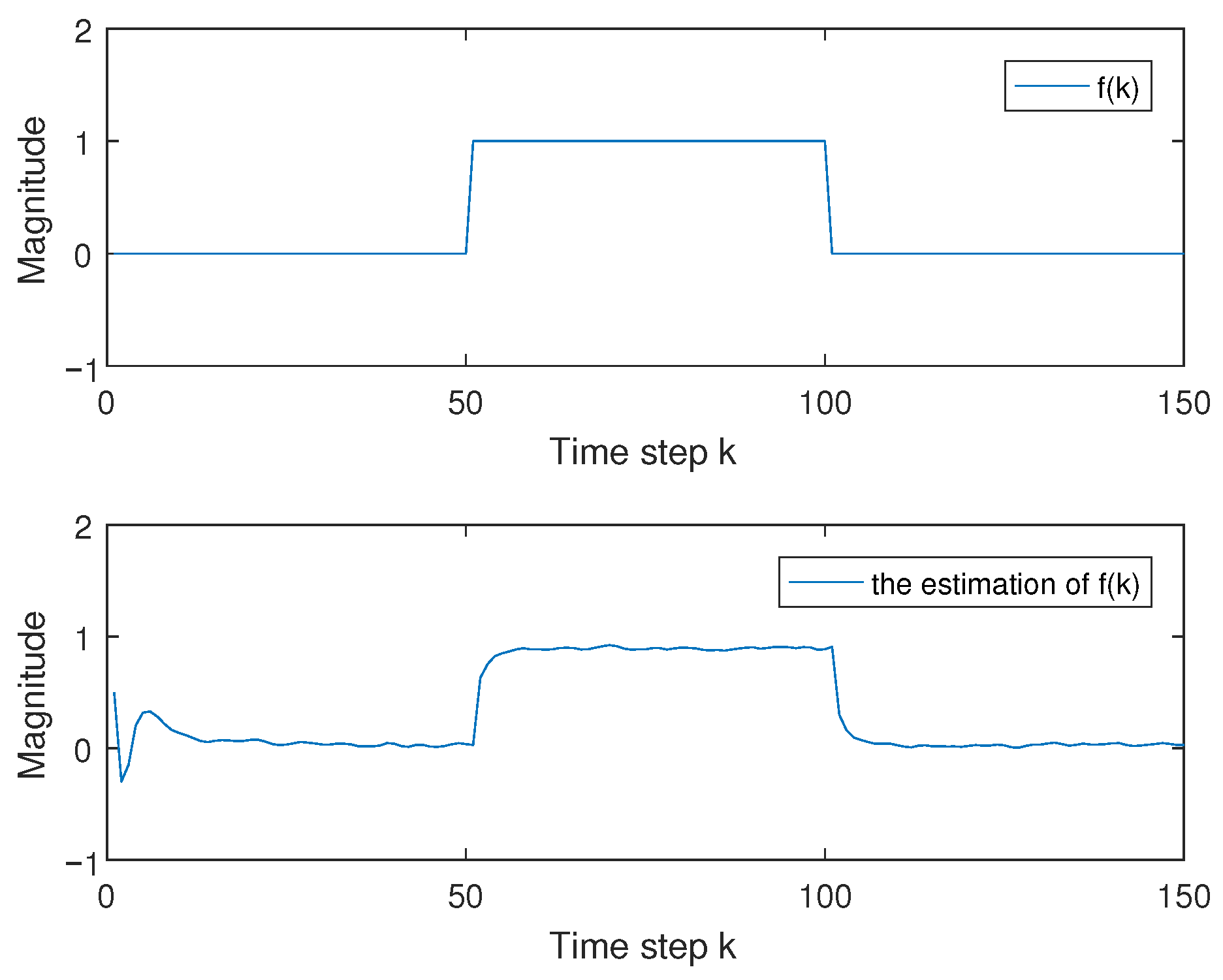
. When
, fault
and its estimation
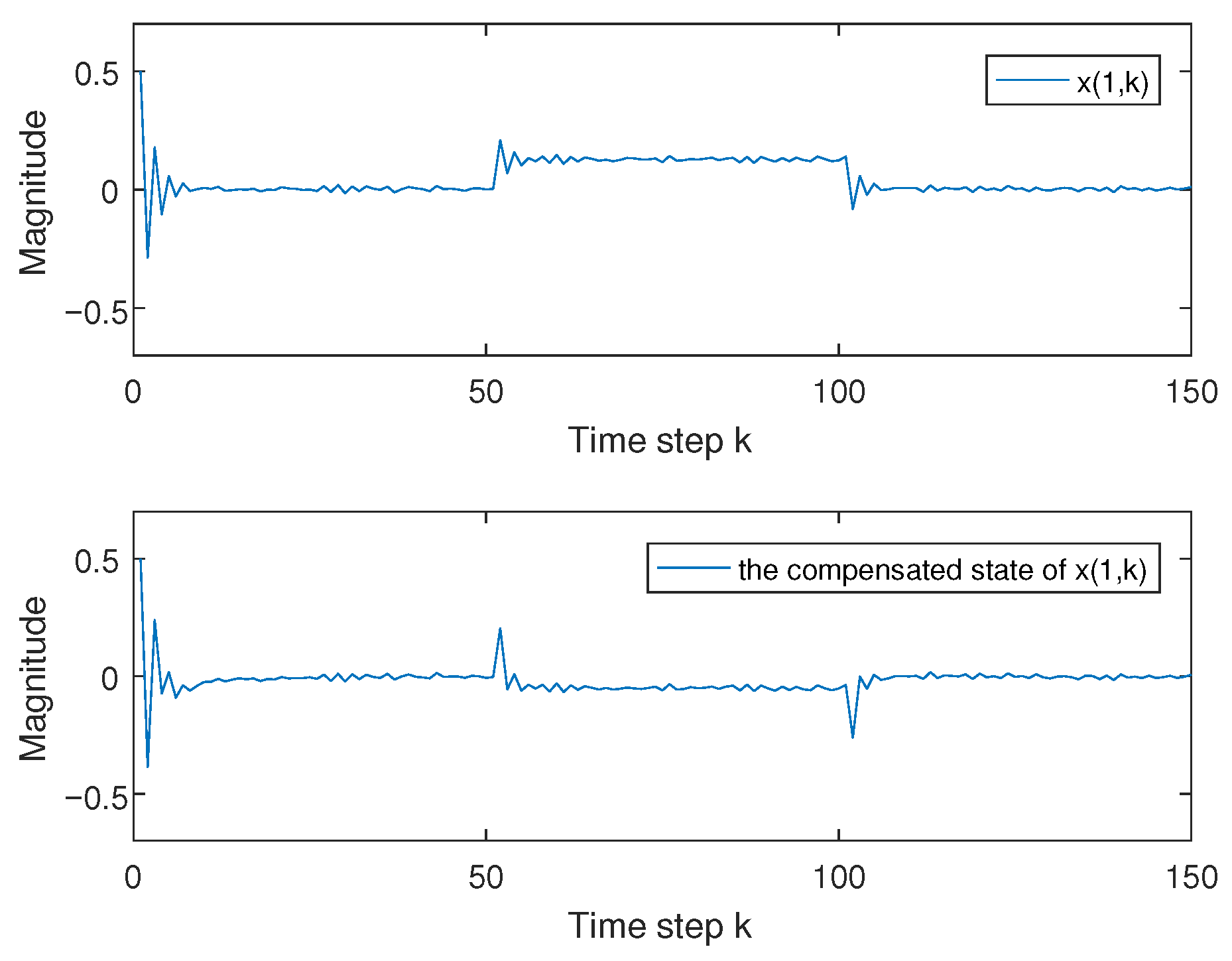
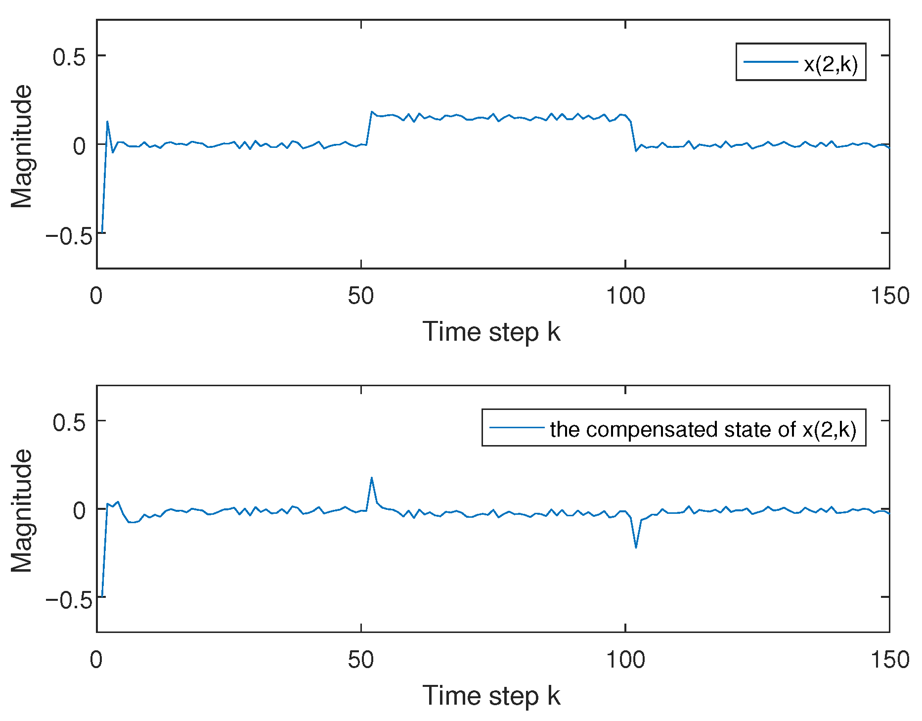
are given in
Figure 1, and the error state in (
5) between system (
1) and system (
3) and its compensated error state are given in
Figure 2 and
Figure 3, which show that controller (
19) is effective by the comparison.
Although this example is a numerical examples, it is easy to obtain that this developed scheme is effective through the above analysis and comparison, i.e., semi-Markov NN has some finite-time -dissipative FTSC ability based on an event-triggered method in this paper.
Remark 6. This paper designs an intermediate observer to estimate faults.
Based on the utilized information, an event-triggered FTSC protocol is proposed to achieve the FTSC with
-dissipativity within finite time. The comparison of this scheme with the existing ones are given in
Table 1.
By this comparison, it is easy to discover that semi-Markov jump discrete NNs in this paper are more consistent with the actual systems. The practicability of this proposed method is better, which is one of our future works.
7. Conclusions
This paper discusses discrete semi-Markov NNs and proposes the finite-time -dissipative FE and FTSC by applying an event-triggered theory. Based on the intermediate variable introduced, an FE scheme is designed to estimate the state, faults, and intermediate variables. Based on the estimate information and the event-triggered condition, an FTSC protocol is constructed to obtain the existence conditions of stochastical finite-time fault-tolerant synchronization with the -dissipativity of error system. The effectiveness of the proposed solution is proven by an example. In future researches, we will mainly study more appropriate FE and FTC design methods to reduce the conservatism and consider their application in engineering practice, such as robot systems, multi-agent systems, UAV swarms, high-speed train traction systems, and so on.
Author Contributions
X.Z.: Conceptualization, methodology, validation, formal analysis, writing, and review and editing. Y.W.: Formal analysis, validation, and editing. Y.C.: Conceptualization, methodology, investigation, resources, and review and editing. All authors have read and agreed to the published version of the manuscript.
Funding
This research was funded by National Natural Science Foundation of China under Grant 62403227, 12201280, and 62273172, and Natural Science Foundation of Shandong Province under Grant ZR2023MF065.
Data Availability Statement
The original contributions presented in this study are included in the article. Further inquiries can be directed to the corresponding author.
Acknowledgments
The authors would like to thank the reviewers for their valuable and helpful comments which have improved the presentation.
Conflicts of Interest
The authors declared that they have no conflicts of interest to this work, or any commercial or associative interest that represents a conflict of interest in connection with the work submitted.
Appendix A
Proof of Theorem 1. Define a Lyapunov functional:
with
. When
, it has
We set
, then
where
Based on Lemma 1, one has
and
Considering Assumption 1, if diagonal matrix
exists, one has
Similarly, it is easy to get
Considering (
18), we can have
with
.
Combined with (
A1)–(
A12), it has
in which
We set
, then
Notice that
, it has
Based on (30) and (31), we have
Based on (32), it has
So system (
25) without
is stochastically fault-tolerant synchronized within finite time.
In the following, we analyse the strict
-
-dissipativity of system (
25) and (26) with
.
When
, it has
Based on (
A3)–(
A9) and (
A20), we have
Considering (
29),
holds. Thus
Summing both side of (
A22) from 0 to
, then
Hence, system (
25) and (26) is strictly
-
-dissipative. That finishes the proof. □
Appendix B
Proof of Theorem 2. Because
in (
29) is nonlinear, we multiply left by
and right by
to (
29),
holds based on Lemma 3, where
. So it has
where
We define
and set
,
, then (
33)–(38) hold based on (
29)–(32). That finishes the proof. □
References
- Zhang, Z.M.; He, Y.; Wu, M.; Wang, Q.G. Exponential synchronization of neural networks with time-varying delays via dynamic intermittent output feedback control. IEEE Trans. Syst. Man Cybern. Syst. 2017, 99, 1–11. [Google Scholar] [CrossRef] [Scilit]
- Zhang, H.Y.; Qiu, Z.P.; Xiong, L.L.; Jiang, G.H. Stochastic stability analysis for neutral-type Markov jump neural networks with additive time-varying delays via a new reciprocally convex combination inequality. Int. J. Syst. Sci. 2017, 5, 970–988. [Google Scholar] [CrossRef] [Scilit]
- Chen, W.Z.; Dai, M.Z.; Guan, C.X.; Fei, Z.Y. Extended dissipativity of semi-Markov jump neural networks with partly unknown transition rates. Neurocomputing 2021, 423, 601–608. [Google Scholar] [CrossRef] [Scilit]
- Wang, Y.; Xia, J.W.; Huang, X.; Zhou, J.P.; Shen, H. Extended disspative synchronization for singularly perturbed semi-Markov jump neural networks with randomly occurring uncertainties. Neurocomputing 2019, 349, 281–289. [Google Scholar] [CrossRef] [Scilit]
- Shen, H.; Wang, Y.; Xia, J.W.; Cao, J.D.; Chen, X.Y. Non-fragile mixed passive and H∞ state estimation for singularly perturbed neural networks with semi-Markov jumping parameters. J. Frankl. Inst. 2020, 357, 6352–6369. [Google Scholar] [CrossRef] [Scilit]
- Rakkiyappan, R.; Maheswari, K.; Velmurugan, G.; Park, J.H. Event-triggered H∞ state estimation for semi-Markov jumping discrete-time neural networks with quantization. Neural Netw. 2018, 105, 236–248. [Google Scholar] [CrossRef] [Scilit]
- Kamenkov, G. On stability of motion over a finite interval of time [in Russian]. J. Appl. Math. Mech. 1953, 17, 529–540. [Google Scholar]
- Yang, P.; Ding, Y.; Shen, Z.W.; Feng, K.J. Integral non-singular terminal sliding mode consensus control for multi-agent systems with disturbance and actuator faults based on finite-time observer. Entropy 2022, 24, 1068. [Google Scholar] [CrossRef] [Scilit] [PubMed]
- Ju, Y.Y.; Cheng, G.F.; Ding, Z.S. Stochastic H∞ finite-time control for linear neutral semi-Markovian jumping systems under event-triggering scheme. J. Frankl. Inst. 2021, 358, 1529–1552. [Google Scholar] [CrossRef] [Scilit]
- Luo, M.H.; Mu, X.W.; Wu, X.H.; Hu, Z.H. Event-triggered non-fragile finite-time H∞ control for semi-Markovian jump systems with actuator saturation. J. Frankl. Inst. 2020, 357, 10626–10647. [Google Scholar] [CrossRef] [Scilit]
- Sun, S.X.; Zhang, H.G.; Li, W.H.; Wang, Y.C. Time-varying delay-dependent finite-time boundedness with H∞ performance for Markovian jump neural networks with state and input constraints. Neurocomputing 2021, 423, 419–426. [Google Scholar] [CrossRef] [Scilit]
- Shen, H.; Park, J.H.; Wu, Z.G. Finite-time synchronization control for uncertain Markov jump neural networks with input constraints. Nonlinear Dyn. 2014, 77, 1709–1720. [Google Scholar] [CrossRef] [Scilit]
- Li, F.; Shen, H.; Chen, M.S.; Kong, Q.K. Non-fragile finite-time l2–l∞ state estimation for discrete-time Markov jump neural networks with unreliable communication links. Appl. Math. Comput. 2015, 271, 467–481. [Google Scholar]
- Li, F.; Shen, H. Finite-time H∞ synchronization control for semi-Markov jump delayed neural networks with randomly occurring uncertainties. Neurocomputing 2015, 166, 447–454. [Google Scholar] [CrossRef] [Scilit]
- Zhang, D.; Cheng, J.; Cao, J.D.; Zhang, D. Finite-time synchronization control for semi-Markov jump neural networks with mode-dependent stochastic parametric uncertainties. Appl. Math. Comput. 2019, 344-345, 230–242. [Google Scholar]
- Wang, J.; Ru, T.T.; Shen, H.; Cao, J.D.; Park, J.H. Finite-time L2-L∞ synchronization for semi-Markov jump inertial neural networks using sampled data. IEEE Trans. Netw. Sci. Eng. 2021, 8, 163–173. [Google Scholar] [CrossRef] [Scilit]
- Niederlinski, A. A heuristic approach to the design of linear multivariable interacting control systems. Automatica 1971, 7, 691–701. [Google Scholar] [CrossRef] [Scilit]
- Liu, L.J.; Lv, J.L.; Lin, H.W.; Zhan, R.D.; Wu, L.M. ADP-based fault-tolerant control with stability guarantee for nonlinear systems. Entropy 2025, 27, 1028. [Google Scholar] [CrossRef] [Scilit]
- Zhu, X.D.; Li, W.Q.; Xia, Y.Q. Finite-time fault estimate and fault-tolerant control for discrete-time Markov jump systems with actuator and sensor faults. Int. J. Robust Nonlinear Control 2023, 33, 6233–6249. [Google Scholar] [CrossRef] [Scilit]
- Wang, Y.; Xia, J.W.; Wang, Z.; Zhou, J.P.; Shen, H. Reliable consensus control for semi-Markov jump multi-agent systems: A leader following strategy. J. Frankl. Inst. 2019, 356, 3612–3627. [Google Scholar] [CrossRef] [Scilit]
- Mu, X.W.; Li, X.; Fang, J.Y.; Wu, X.H. Reliable observer-based finite-time H∞ control for networked nonlinear semi-Markovian jump systems with actuator fault and parameter uncertainties via dynamic event-triggered scheme. Inf. Sci. 2021, 546, 573–595. [Google Scholar] [CrossRef] [Scilit]
- Wang, J.; Shen, H. Passivity-based fault-tolerant synchronization control of chaotic neural networks against actuator faults using the semi-Markov jump model approach. Neurocomputing 2014, 143, 51–56. [Google Scholar] [CrossRef] [Scilit]
- Zhou, J.P.; Liu, Y.M.; Xia, J.W.; Wang, Z.; Arikd, S. Resilient fault-tolerant anti-synchronization for stochastic delayed reaction-diffusion neural networks with semi-Markov jump parameters. Neural Netw. 2020, 125, 194–204. [Google Scholar] [CrossRef] [Scilit] [PubMed]
- Wang, Z.; Liu, Y.; Yu, L.; Liu, X. Exponential stability of delayed recurrent neural networks with Markovian jumping parameters. Phys. Lett. A 2006, 356, 346–352. [Google Scholar] [CrossRef] [Scilit]
- Zhu, J.; Yang, G.; Wang, H.; Wang, F. Fault estimation for a class of nonlinear systems based on intermediate estimator. IEEE Trans. Autom. Control 2016, 61, 2518–2524. [Google Scholar] [CrossRef] [Scilit]
- Zhu, J.; Yang, G. Robust distributed fault estimation for a network of dynamical systems. IEEE Trans. Control Netw. Syst. 2018, 5, 14–22. [Google Scholar] [CrossRef] [Scilit]
- Han, J.; Liu, X.H.; Gao, X.W.; Wei, X.J. Intermediate observer based robust distributed fault estimation for nonlinear multi-agent systems with directed graphs. IEEE Trans. Ind. Inform. 2020, 16, 7426–7436. [Google Scholar] [CrossRef] [Scilit]
- Liu, X.X.; Su, X.J.; Shi, P.; Nguang, S.K.; Shen, C. Fault detection filtering for nonlinear switched systems via event-triggered communication approach. Automatica 2019, 101, 365–376. [Google Scholar] [CrossRef] [Scilit]
- Zuo, Z.; Liu, Y.; Wang, Y.; Li, H. Finite–time stochastic stability and stabilisation of linear discrete-time Markovian jump systems with partly unknown transition probabilities. IET Control Theory Appl. 2012, 6, 1522–1526. [Google Scholar] [CrossRef] [Scilit]
- Shi, P.; Su, X.J.; Li, F.B. Dissipativity-based filtering for fuzzy switched systems with stochastic perturbation. IEEE Trans. Autom. Control 2016, 61, 1694–1699. [Google Scholar] [CrossRef] [Scilit]
- Wang, Y.; Xie, L.; Souza, C.E.D. Robust control of a class of uncertain nonlinear systems. Syst. Control Lett. 1992, 19, 139–149. [Google Scholar] [CrossRef] [Scilit]
- Gu, K.; Chen, J.; Kharitonov, V.L. Stability of Time-Delay Systems; Springer Science and Business Media: Berlin/Heidelberg, Germany, 2003. [Google Scholar]
- Xiong, J.; Lam, J. Stabilization of networked control systems with a logic ZOH. IEEE Trans. Autom. Control 2009, 54, 358–363. [Google Scholar] [CrossRef] [Scilit]
- Li, F.B.; Wu, L.G.; Shi, P. Stochastic stability of semi-Markovian jump systems with mode-dependent delays. Int. J. Robust Nonlinear Control 2014, 24, 3317–3330. [Google Scholar] [CrossRef] [Scilit]
| Disclaimer/Publisher’s Note: The statements, opinions and data contained in all publications are solely those of the individual author(s) and contributor(s) and not of MDPI and/or the editor(s). MDPI and/or the editor(s) disclaim responsibility for any injury to people or property resulting from any ideas, methods, instructions or products referred to in the content. |
© 2025 by the authors. Licensee MDPI, Basel, Switzerland. This article is an open access article distributed under the terms and conditions of the Creative Commons Attribution (CC BY) license (https://creativecommons.org/licenses/by/4.0/).