

Boosted Binary Quantum Classifier via Graphical Kernel


Abstract
1. Introduction
2. Quantum Machine Learning Based on Graphical Feature Space
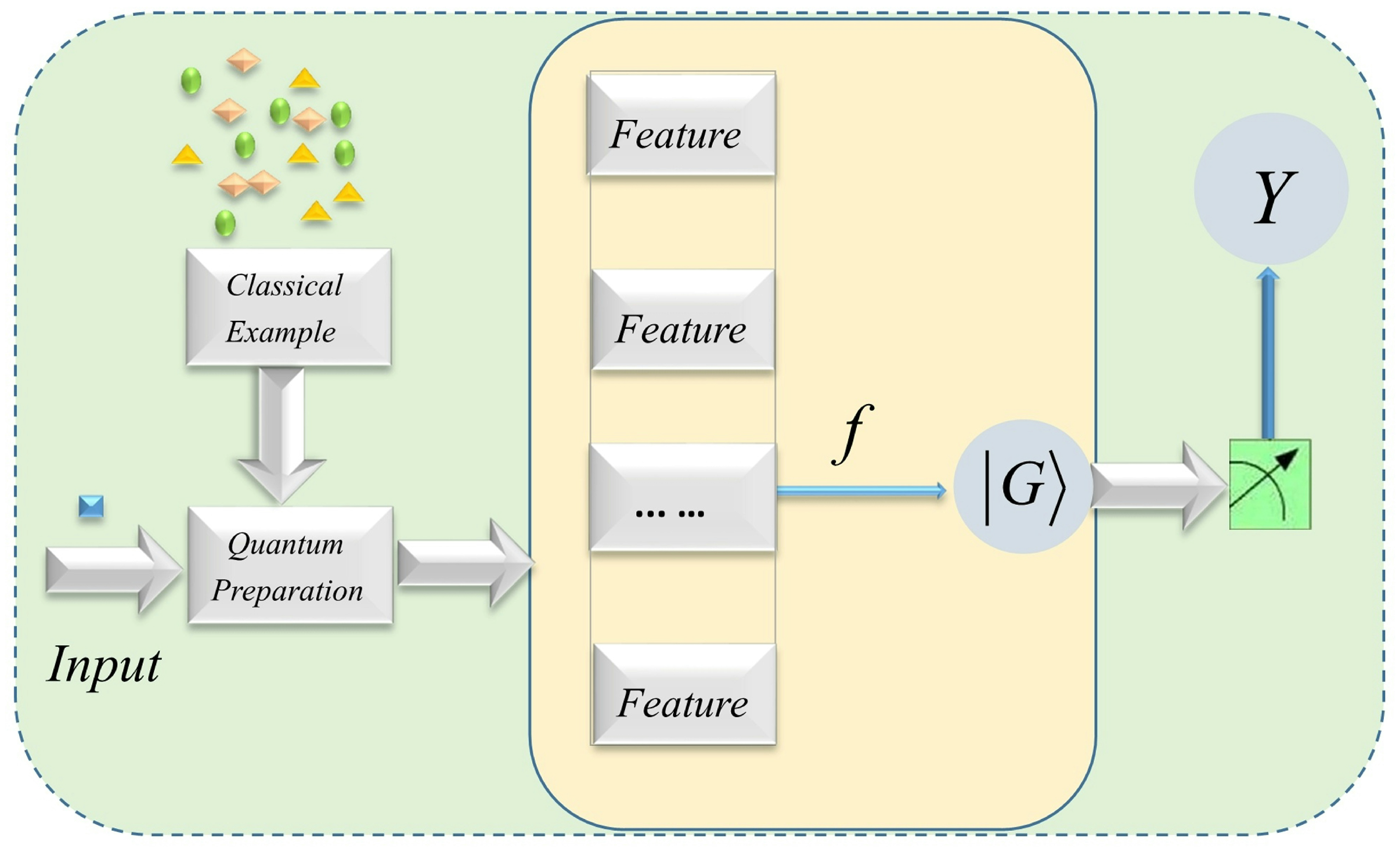
2.1. The Basic Map of Feature Space in Quantum Machine Learning
2.2. Two-Level Quantum Nested Graphical States Mapped to Feature Space
3. Swap-Test Quantum Classifier with Large-Scale Data
3.1. Quantum Swap-Test Classification Based on Graph State
3.2. Quantum Graph Kernels and Graph Segmentation
3.3. Fidelity Analysis in Quantum Classifiers
4. Experiments
4.1. Algorithm
| Algorithm 1: Quantum classifier with respect to quantum encoding |
Prepare: Sample set X, unlabeled test point and quantum classifier circuit . Input: graph , adjacent matrix 1. for , do encode into with quantum phase encoder. 2. Applying H to entangle the sample states with , so that two-level graph state coupling graph is formed. 3. Resort to the circuit , fordo obtain M classes of weak quantum classifiers . 4. Computing the distances between and Output: The label y that belongs to. |
4.2. Boosted Classification Algorithm and Comparison
| Algorithm 2: Boosted quantum classifier with T cycles |
Input: Quantum training dataset ; weak learning algorithm ; integer T of iterative cycle; form sample state vector and ancilla vector Initialize the weight of graph for , and for, do 1. Construct cluster states and 2. Compute mixed state to obtain 3. Apply to provide , return . 4. Obtain the error of . 5. Update weights vector Output: the of graph state . |
4.3. Running Time Analysis
5. Conclusions
Author Contributions
Funding
Institutional Review Board Statement
Data Availability Statement
Conflicts of Interest
References
- Nielsen, M.; Aand Chuang, I.S. Quantum Computation and Quantum Information; Cambridge University Press: Cambridge, UK, 2000. [Google Scholar]
- Cirac, J.I.; Zoller, P. Scalable quantum computer with ions in an array of microtraps. Nature 2000, 404, 579–581. [Google Scholar] [CrossRef] [PubMed]
- Sasaki, M.; Carlini, A. Quantum learning and universal quantum matching machine. Phys. Rev. A 2002, 66, 022303. [Google Scholar] [CrossRef]
- Rebentrost, P.; Mohseni, M.; Lloyd, S. Quantum support vector machine for big data classification. Phys. Rev. Lett. 2014, 113, 130503. [Google Scholar] [CrossRef] [PubMed]
- Lu, S.; Braunstein, S.L. Quantum decision tree classifier. Quantum Inf. Process. 2014, 13, 757–770. [Google Scholar] [CrossRef]
- Hu, W. Comparison of Two Quantum Nearest Neighbor Classifiers on IBM’s Quantum Simulator. Nat. Sci. 2018, 10, 87–98. [Google Scholar] [CrossRef]
- Biamonte, J.; Wittek, P.; Pancotti, N.; Rebentrost, P.; Wiebe, N.; Lloyd, S. Quantum machine learning. Nature 2017, 549, 195. [Google Scholar] [CrossRef]
- Blank, C.; Park, D.K.; Rhee, J.K.K.; Petruccione, F. Quantum classifier with tailored quantum kernel. npj Quantum Inf. 2020, 6, 41. [Google Scholar] [CrossRef]
- Du, Y.; Hsieh, M.H.; Liu, T.; Tao, D. A Grover-search based quantum learning scheme for classification. New J. Phys. 2021, 23, 023020. [Google Scholar] [CrossRef]
- Liao, H.; Convy, I.; Huggins, W.J.; Whaley, K.B. Robust in practice: Adversarial attacks on quantum machine learning. Phys. Rev. A 2021, 103, 042427. [Google Scholar] [CrossRef]
- Li, Y.; Meng, Y.; Luo, Y. Quantum Classifier with Entangled Subgraph States. Int. J. Theor. Phys. 2021, 60, 3529–3538. [Google Scholar] [CrossRef]
- Zhou, N.R.; Zhang, T.F.; Xie, X.W.; Wu, J.Y. Hybrid quantum Cclassical generative adversarial networks for image generation via learning discrete distribution. Signal Process. Image Commun. 2023, 110, 116891. [Google Scholar] [CrossRef]
- Briegel, H.J.; Raussendorf, R. A One-Way Quantum Computer. Phys. Rev. Lett. 2001, 86, 910. [Google Scholar] [CrossRef] [PubMed]
- Mandel, O.; Greiner, M.; Widera, A.; Rom, T.; Hnsch, T.W.; Bloch, I. Controlled collisions for multi-particle entanglement of optically trapped atoms. Nature 2003, 425, 937. [Google Scholar] [CrossRef] [PubMed]
- Raussendorf, R.; Browne, D.E.; Briegel, H.J. Measurement-based quantum computation using cluster states. Phys. Rev. A 2003, 68, 022312. [Google Scholar] [CrossRef]
- Dür Aschauer, W.H.; Briegel, H.J. Multiparticle Entanglement Purification for Graph States. Phys. Rev. Lett. 2003, 91, 107903. [Google Scholar]
- Walther, P.; Pan, J.W.; Aspelmeyer, M.; Ursin, R.; Gasparoni, S.; Zeilinger, A. De Broglie wavelength of a non-local four-photon state. Nature 2004, 429, 158. [Google Scholar] [CrossRef]
- Hein, M.; Eisert, J.; Briegel, H.J. Multi-party entanglement in graph states. Phys. Rev. A 2004, 69, 062311. [Google Scholar] [CrossRef]
- Clark, S.R.; Alves, C.M.; Jaksch, D. Efficient generation of graph states for quantum computation. New J. Phys. 2005, 7, 124. [Google Scholar] [CrossRef]
- Aschauer, H.; Dur, W.; Briegel, H.J. Multiparticle entanglement purification for two-colorable graph states. Phys. Rev. A 2005, 71, 012319. [Google Scholar] [CrossRef]
- Hu, D.; Tang, W.; Zhao, M.; Chen, Q.; Yu, S.; Oh, C.H. Graphical Nonbinary Quantum Error-Correcting Codes. Phys. Rev. A 2008, 78, 012306. [Google Scholar] [CrossRef]
- Park, D.K.; Petruccione, F.; Rhee, J.K.K. Circuit-based quantum random access memory for classical data. Sci. Rep. 2019, 9, 3949. [Google Scholar] [CrossRef]
- Schuld, M.; Petruccione, F. Supervised Learning with Quantum Computers; Springer: Cham, Switzerland, 2018. [Google Scholar]
- Schuld, M.; Sinayskiy, I.; Petruccione, F. An introduction to quantum machine learning. Contemp. Phys. 2015, 56, 172–185. [Google Scholar] [CrossRef]
- Esma, A.; Gilles, B.; Seebastien, G. Machine learning in a quantum world. In Advances in Artificial Intelligence; Springer: Berlin/Heidelberg, Germany, 2006; pp. 431–442. [Google Scholar]
- Wittek, P. Quantum Machine Learning: What Quantum Computing Means to Data Mining; Academic Press: Boston, MA, USA, 2014. [Google Scholar]
- Pudenz, K.L.; Lidar, D.A. Quantum adiabatic machine learning Quantum. Quant. Inf. Proc. 2013, 12, 2027. [Google Scholar] [CrossRef]
- Turkpence, D.; Akncß, T.Ç.; Şeker, S. A steady state quantum classifier. Phys. Lett. A 2019, 383, 1410–1418. [Google Scholar] [CrossRef]
- Schuld, M.; Fingerhuth, M.; Petruccione, F. Implementing a distance-based classifier with a quantum interference circuit. EPL (Europhys. Lett.) 2017, 119, 60002. [Google Scholar] [CrossRef]
- Danielsen, L.E. On self-dual quantum codes, graphs, and Boolean functions. arXiv 2005, arXiv:0503236. [Google Scholar]
- Li, Y.; Ji, C.L.; Xu, M.T. Nested Quantum Error Correction Codes via Subgraphs. Int. J. Theor. Phys. 2014, 53, 390–396. [Google Scholar] [CrossRef]
- Gottesman, D. Class of quantum error-correcting codes saturating the quantum Hamming bound. Phys. Rev. A 1996, 54, 1862–1868. [Google Scholar] [CrossRef]
- Calderbank, A.R.; Rains, E.M.; Shor, P.W.; Sloane, N.J. Quantum error correction and orthogonal geometry. Phys. Rev. Lett. 1997, 76, 405–409. [Google Scholar] [CrossRef]
- Calderbank, A.R.; Shor, P. Good quantum error-correcting codes exist. Phys. Rev. A 1996, 54, 1098–1105. [Google Scholar] [CrossRef]
- Cong, I.; Choi, S.; Lukin, M.D. Quantum convolutional neural networks. Nat. Phys. 2019, 15, 1273–1278. [Google Scholar] [CrossRef]
- Huang, H.Y.; Broughton, M.; Mohseni, M.; Babbush, R.; Boixo, S.; Neven, H.; McClean, J.R. Power of data in quantum machine learning. Nat. Commun. 2021, 12, 2631. [Google Scholar] [CrossRef] [PubMed]
- Schuld, M.; Bradler, K.; Israel, R.; Su, D.; Gupt, B. Measuring the similarity of graphs with a gaussian boson sampler. Phys. Rev. A 2020, 101, 032314. [Google Scholar] [CrossRef]
- IBM. Quantum Experience. Available online: www.research.ibm.com/quantum (accessed on 21 September 2022).
- Qiskit. Available online: https://qiskit.org/ (accessed on 14 November 2019).
- Fisher, P.A. The use of multiple measurements in taxonomic problems. Ann. Eugen. 1936, 7, 179–188. [Google Scholar] [CrossRef]
- Aaronson, S. Quantum Machine Learning Algorithms: Read the Fine Print. arXiv 2009, arXiv:0910.4698. [Google Scholar]


| Dataset | Qubits | Cycle | Experimental (%) | Simulation (%) |
|---|---|---|---|---|
| Iris | 5 | 1 | 83.51 | 87.92 |
| 2 | 96.20 | 97.58 | ||
| 3 | 98.37 | 98.86 | ||
| Skin | 5 | 1 | 67.33 | 73.54 |
| 2 | 76.46 | 79.59 | ||
| 3 | 83.12 | 84.85 |
| Dataset | Model | Method | Precision (%) | Recall (%) | F1-Measure (%) | Qubit Error |
|---|---|---|---|---|---|---|
| Iris | Classical Model | KNN | 94.12 | 94.06 | 94.09 | |
| SVM | 93.54 | 93.26 | 93.40 | |||
| Decision Trees | 93.82 | 94.01 | 93.91 | |||
| Quantum Model | QBoosting | 95.34 | 96.06 | 95.70 | 0.0183 | |
| QKNN | 94.67 | 95.56 | 95.11 | 0.0192 |
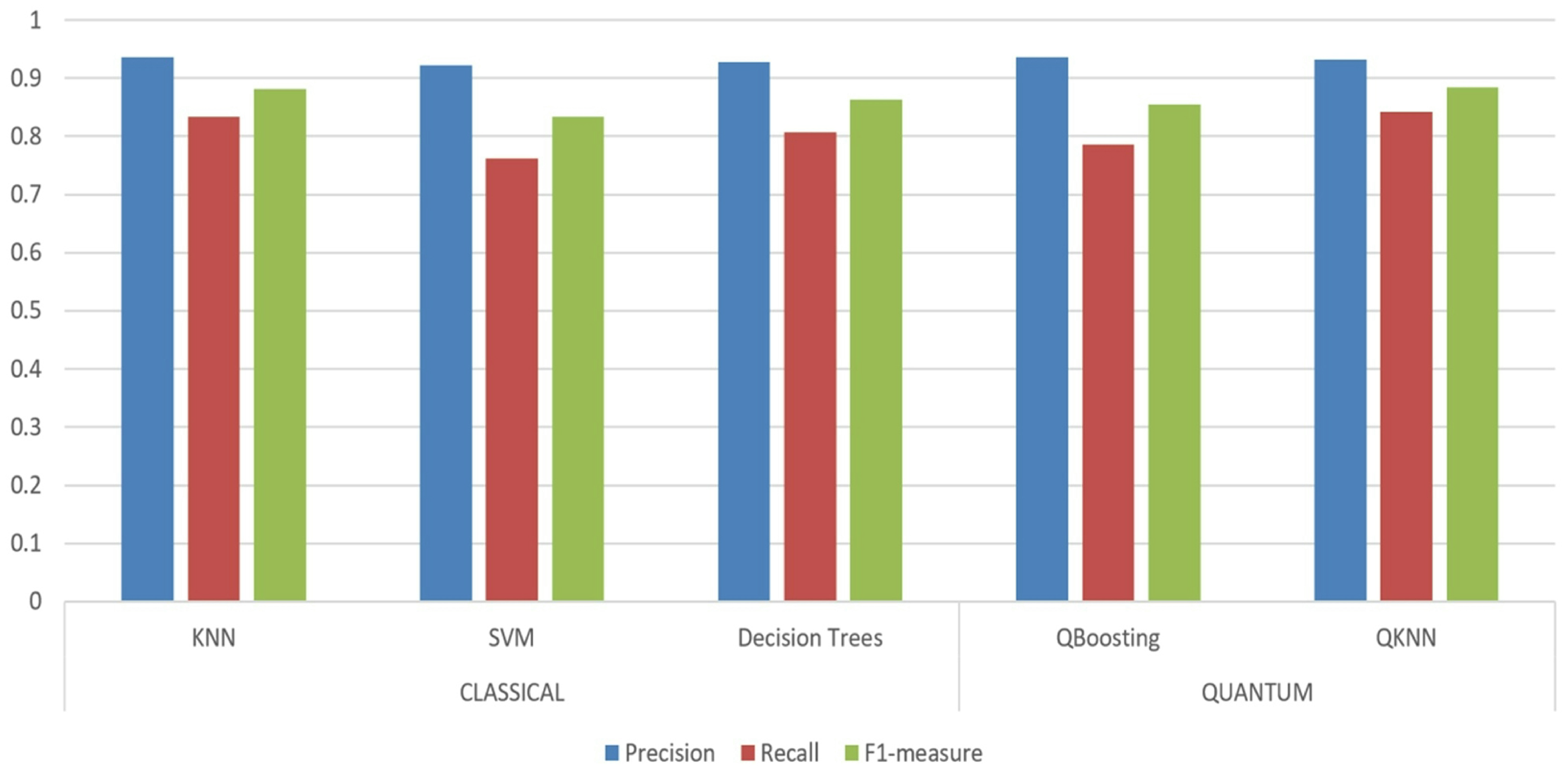
| Dataset | Model | Method | Precision (%) | Recall (%) | F1-Measure (%) | Qubit Error |
|---|---|---|---|---|---|---|
| Skin | Classical Model | KNN | 93.54 | 83.41 | 88.19 | |
| SVM | 92.23 | 76.13 | 83.41 | |||
| Decision Trees | 92.78 | 81.62 | 86.30 | |||
| Quantum Model | QBoosting | 93.57 | 78.57 | 85.42 | 0.0327 | |
| QKNN | 93.21 | 84.13 | 88.43 | 0.0438 |
Disclaimer/Publisher’s Note: The statements, opinions and data contained in all publications are solely those of the individual author(s) and contributor(s) and not of MDPI and/or the editor(s). MDPI and/or the editor(s) disclaim responsibility for any injury to people or property resulting from any ideas, methods, instructions or products referred to in the content. |
© 2023 by the authors. Licensee MDPI, Basel, Switzerland. This article is an open access article distributed under the terms and conditions of the Creative Commons Attribution (CC BY) license (https://creativecommons.org/licenses/by/4.0/).
Share and Cite
Li, Y.; Huang, D. Boosted Binary Quantum Classifier via Graphical Kernel. Entropy 2023, 25, 870. https://doi.org/10.3390/e25060870
Li Y, Huang D. Boosted Binary Quantum Classifier via Graphical Kernel. Entropy. 2023; 25(6):870. https://doi.org/10.3390/e25060870
Chicago/Turabian StyleLi, Yuan, and Duan Huang. 2023. "Boosted Binary Quantum Classifier via Graphical Kernel" Entropy 25, no. 6: 870. https://doi.org/10.3390/e25060870
APA StyleLi, Y., & Huang, D. (2023). Boosted Binary Quantum Classifier via Graphical Kernel. Entropy, 25(6), 870. https://doi.org/10.3390/e25060870