
Quantum Lernmatrix


Department of Computer Science and Engineering, INESC-ID & Instituto Superior Técnico, University of Lisbon, 2740-122 Porto Salvo, Portugal
Entropy 2023, 25(6), 871; https://doi.org/10.3390/e25060871
Submission received: 28 March 2023
/
Revised: 25 May 2023
/
Accepted: 26 May 2023
/
Published: 29 May 2023
(This article belongs to the Special Issue Quantum Machine Learning 2022)
Abstract
We introduce a quantum Lernmatrix based on the Monte Carlo Lernmatrix in which n units are stored in the quantum superposition of units representing binary sparse coded patterns. During the retrieval phase, quantum counting of ones based on Euler’s formula is used for the pattern recovery as proposed by Trugenberger. We demonstrate the quantum Lernmatrix by experiments using qiskit. We indicate why the assumption proposed by Trugenberger, the lower the parameter temperature t; the better the identification of the correct answers; is not correct. Instead, we introduce a tree-like structure that increases the measured value of correct answers. We show that the cost of loading L sparse patterns into quantum states of a quantum Lernmatrix are much lower than storing individually the patterns in superposition. During the active phase, the quantum Lernmatrices are queried and the results are estimated efficiently. The required time is much lower compared with the conventional approach or the of Grover’s algorithm.
1. Introduction
There are two popular models of quantum associative memories, the quantum associative memory as proposed by Venture and Martinez [1,2,3] and the quantum associative memory as proposed by Trugenberger [4,5]. Both models store binary patterns represented by linear independent vectors by basis encoding. They prepare the linear independent states by a procedure that is based on dividing present superposition into processing and memory terms flagged by an ancilla bit. New input patterns are successively loaded into the processing branch that is divided by a parametrized controlled-U operation on an ancilla and then the pattern is merged, resulting in a superposition of linear independent states. The method is linear in the number of stored patterns and their dimension [6].
In the quantum associative memory as proposed by Venture and Martinez, a modified version of Grover’s search algorithm [7,8,9,10], ref. [7] is applied to determine the answer vector to a query vector [1,2,3]. In Trugenberger’s model, the retrieval mechanism is based on Euler’s formula to determine if the input pattern is similar to the set of stored patterns. In an additional step, the most similar pattern can be estimated by the introduced temperature parameter or alternatively by the Grover’s search algorithm. Both models suffer from the problem of input destruction (ID problem) [11,12,13]:
- The input (reading) problem: The amplitude distribution of a quantum state is initialized by reading n data points. Although the existing quantum algorithm requires only steps or and is faster than the classical algorithms, n data points must be read. Hence, the complexity of the algorithm does not improve and is .
- The destruction problem: A quantum associative memory [1,2,3,4,5] for n data points for dimension m requires only or fewer units (quantum bits). An operator, which acts as an oracle [3], indicates the solution. However, this memory can be queried only once because of the collapse during measurement (destruction); hence, quantum associative memory does not have any advantages over classical memory.
Most quantum machine learning algorithms suffer from the input destruction problem [13]. Trugenberger tries to overcome the destruction problem by the probabilistic cloning of the quantum associative memory [4,14]. This approach was criticized in [15]. The efficient preparation of data is possible in part for spare data [16]. However, the input destruction problem is not solved till today, and usually theoretical speed ups are analyzed [17] by ignoring the input problem, which is the main bottleneck for data encoding.
In our approach, the preparation costs in which data points must be read and the query time are represented by two phases that are analyzed independently. As in the Harrow [16] approach, our data are sparse. The sparse data are stored in the best possible distributed compression methods [18,19] by a Lernmatrix [20,21] also called Willshaw’s associative memory [22]. Our quantum Lernmatrix model is based on the Lernmatrix.
We prepare a set of quantum Lernmatrices in superposition. This preparation requires a great deal of time and we name it the sleep phase. On the other hand, in the active phase, the query operation is extremely fast. The cost of the sleep phase and the active phase are the same as one of a conventional Lernmatrix. We assume that in the sleep phase we have enough time to prepare several quantum Lernmatrices in superposition.
The quantum Lernmatrices are kept in superposition until they are queried in the active phase. Each of the copies of the quantum Lernmatrix can be queried only one time due to the destruction problem. We argue that the advantage to conventional associative memories is present in the active phase where the fast determination of information is essential. The naming of the phases is in analogy to a living organism that prepares itself during the sleep for an active day.
The quantum Lernmatrix does not store independent vectors, but units that represent the compressed binary patterns. The units are described by binary weight vectors that can be correlated, so we cannot use the approach as proposed by Venture, Martinez and Trugenberger. Instead, we prepare the superposition of the weight vectors of the units by the entanglement of index qubits in superposition with the weight vectors. The retrieval phase is based on Euler’s formula as suggested by Trugenberger [4,14]. However, we do not determine the Hamming distance to the query vector, but the number of ones of the query vector that are present in the weight vector. We indicate the quantum Lernmatrix qiskit implementation step by step. Qiskit is an open-source software development kit (SDK) for working with quantum computers at the level of circuits and algorithms from IBM [23]. The paper is organized as follows:
- We introduce the Lernmatrix model described by units that model neurons.
- We indicate that Lernmatrix has a tremendous storage capacity, much higher than most other associative memories. This is valid for sparse equally distributed ones in vectors representing the information.
- Quantum counting of ones based on Euler’s formula is described.
- Based on the Lernmatrix model, a quantum Lernmatrix is introduced in which units are represented in superposition and the query operation is based on quantum counting of ones. The measured result is a position of a one or zero in the answer vector.
- We analyze the Trugenberger amplification.
- Since a one in the answer vector represents information, we assume in that we can reconstruct the answer vector by measuring several ones, taking for granted that the rest of the vector is zero. In a sparse code with k ones, k measurements of different ones reconstruct the binary answer vector. We can increase the probability of measuring a one by the introduced tree-like structure.
- The Lernmatrix can store much more patterns then the number of units. Because of this, the cost of loading L patterns into quantum states is much lower than storing the patterns individually.
2. Lernmatrix
Associative memory models human memory [24,25,26,27,28]. The associative memory and distributed representation incorporate the following abilities in a natural way [18,28,29,30]:
- The ability to correct faults if false information is given.
- The ability to complete information if some parts are missing.
- The ability to interpolate information. In other words, if a sub-symbol is not currently stored, the most similar stored sub-symbol is determined.
Different associative memory models have been proposed over the years [19,28,31,32,33]. The Hopfield model represents a recurrent model of the associative memory [29,31,34], it is a dynamical system that evolves until it has converged to a stable state. The Lernmatrix, or Willshaw’s associative memory, also simply called “associative memory” (if no confusion with other models is possible [32,33]), it was developed by Steinbuch in 1958 as a biologically inspired model from the effort to explain the psychological phenomena of conditioning [20,21]. The goal was to produce a network that could use a binary version of Hebbian learning to form associations between pairs of binary vectors. Later, this model was studied under biological and mathematical aspects mainly by Willshaw [22] and Palm [18,24] and it was shown that this simple model has a tremendous storage capacity.
Lernmatrix is composed of a cluster of units. Each unit represents a simple model of a real biological neuron. Each unit is composed of binary weights, which correspond to the synapses and dendrites in a real neuron (see Figure 1).
They are described by in Figure 2. T is the threshold of the unit.
The presence of a feature is indicated by a “one” component of the vector, its absence through a “zero” component of the vector. A pair of these vectors is associated and this process of association is called learning. The first of the two vectors is called the query vector and the second, the answer vector. After learning, the query vector is presented to the associative memory and the answer vector is determined by the retrieval rule.
2.1. Learning and Retrieval
Initially, no information is stored in the associative memory. Because the information is represented in weights, all unit weights are initially set to zero. In the learning phase, pairs of binary vector are associated. Let be the query vector and the answer vector, the learning rule is:
This rule is called the binary Hebbian rule [18]. Every time a pair of binary vectors is stored, this rule is used.
In the one-step retrieval phase of the associative memory, a fault tolerant answering mechanism recalls the appropriate answer vector for a query vector .
The retrieval rule for the determination of the answer vector is:
where T is the threshold of the unit. The threshold T is set to the number of “one” components in the query vector , . If the output of the unit is 1, we say that the units fires, and for the output 0 the unit does not fire. The cost of the one-step retrieval is . The retrieval is called:
- Hetero-association if both vectors are different ,
- Association, if , the answer vector represents the reconstruction of the disturbed query vector.
For simplicity, we assume that the dimension of the query vector and the answer vector are the same, .
Example
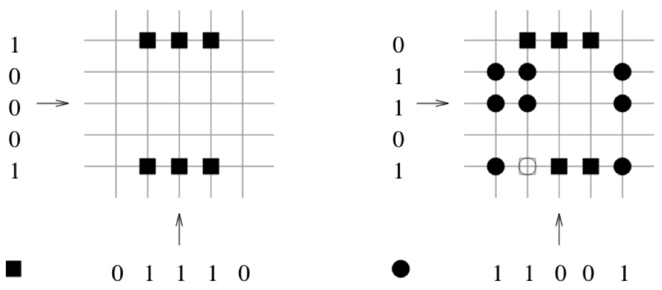
In Figure 3 the vector pair and is learned. The corresponding binary weights of the associated pair are indicated by a black square. In the next step, the vector pair and is learned. The corresponding binary weights of the associated pair are indicated by a black circle. In the third step, the retrieval phase is preformed (see Figure 4). The query vector differs by one bit to the learned query vector . The threshold T is set to the number of “one” components in the query vector , . The retrieved vector is the vector that was stored.
2.2. Storage Capacity
We analyze the optimal storage costs of the Lernmatrix. For an estimation of the asymptotic number L of vector pairs that can be stored in an associative memory before it begins to make mistakes in the retrieval phase, it is assumed that both vectors have the same dimension n. It is also assumed that both vectors are composed of k ones, which are equally likely to be in any coordinate of the vector. In this case, it was shown [18,19,38] that the optimum value for k is approximately
For example, for a vector of the dimension n = 1,000,000, only ones should be used to code a pattern according to the Equation (3). For an optimal value for k according to the Equation (3) with ones equally distributed over the coordinates of the vectors, approximately L vector pairs can be stored in the associative memory [18,19]. L is approximately
This value is much greater than n. The estimate of L is very rough because Equation (3) is only valid for very large networks; however, the capacity increase is still considerable. The upper bound for large n is
the asymptotic capacity is percent per bit, which is much higher than most associative memories. This capacity is only valid for sparse equally distributed ones [18]. The promise of Willshaw’s associative memory that it can store much more patterns then the number of units. The cost of loading patterns in n units with is . It is much lower than storing the L patterns in a list of L units This is because , or
since
The Lernmatrix has a tremendous storage capacity [18,19], it can store much more patterns then the number of units.
The description of how to generated efficiently binary sparse codes of visual patterns or other data structure is described in [39,40,41]. For example, real vector patterns have to be binarized.
The asymptotic capacity is per bit, which is much higher than most associative memories. This capacity is only valid for sparse equally distributed ones [18]. The description of how to generate efficiently binary sparse codes of visual patterns or other data structures is described in [39,40,41]. For example, real vector patterns have to be binarized.
2.3. Large Matrices
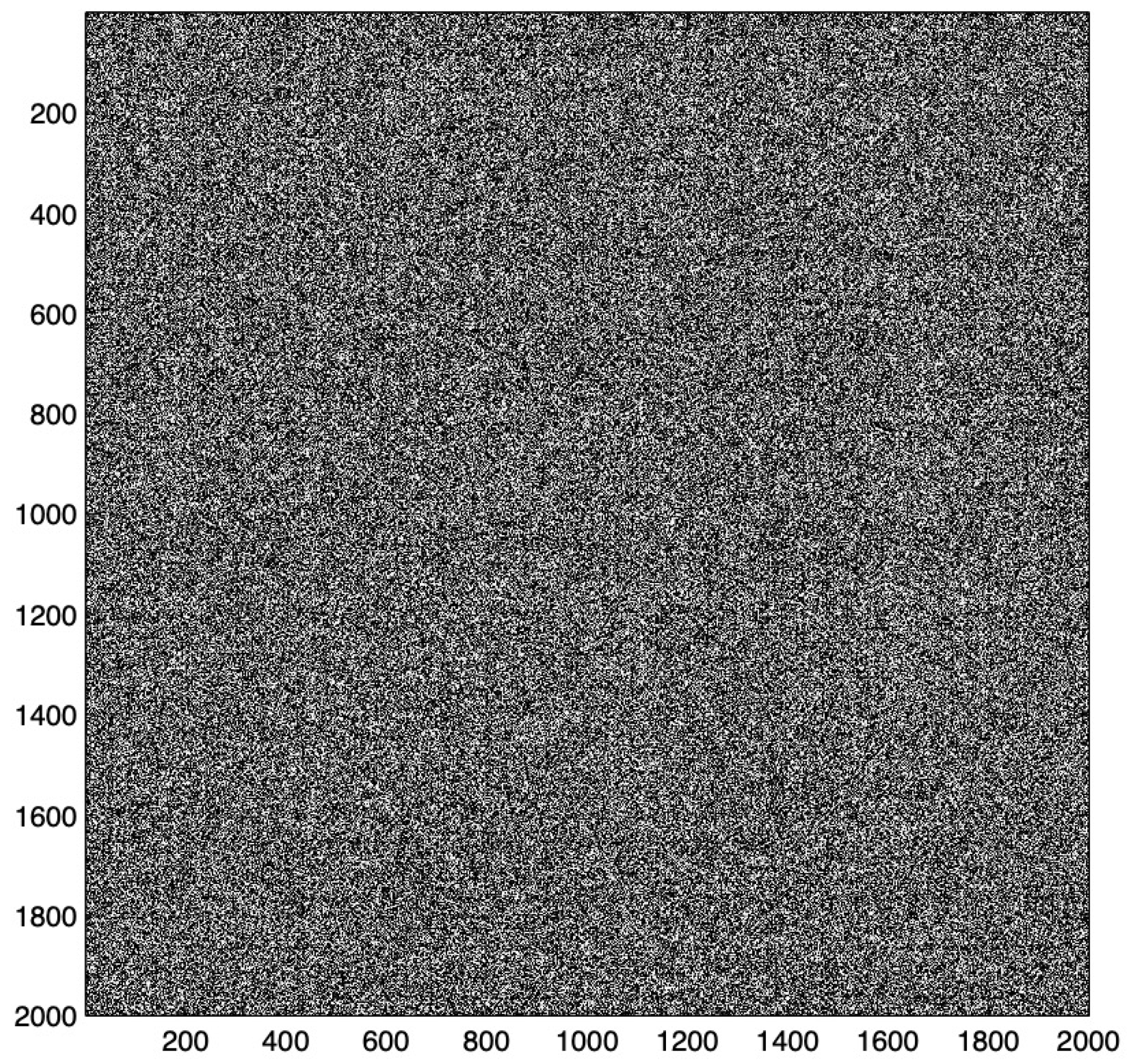
The diagram of the weight matrix illustrates the weight distribution, which results from the distribution of the stored patterns [42,43]. Useful associative properties result from equally distributed weights over the whole weight matrix and are only present in large matrices. A high percentage indicates an overload and the loss of its associative properties. Figure 5 represents a diagram of a high loaded matrix with equally distributed weights.
3. Monte Carlo Lernmatrix
The suggested probabilistic retrieval rule for the determination of the answer vector for the query vector is
and
describing the probability of firing or not firing of one unit with
During the query operation one unit is randomly sampled and either it fires or not according to the probability distribution. To determine the answer vector, we have to sample the Monte Carlo Lernmatrix several times. For the reconstructed vector three states will be present: 1 for fired units, 0 for not fired units and for silent units. The Monte Carlo Lernmatrix is a close description of the quantum Lernmatrix. In the quantum Lernmatrix, units are represented by quantum states, with sampling correspond to the measurement.
4. Qiskit Experiments
Qiskit is an open-source software development kit (SDK) for working with quantum computers at the level of circuits and algorithms [23], IBM Quantum, https://quantum-computing.ibm.com/ (accessed on 25 May 2023 ), 2023, Qiskit (Version 0.43.0). Qiskit provides tools for creating and manipulating quantum programs and running them on prototype quantum devices on the IBM Quantum Experience or on simulators on a local computer. It follows the quantum circuit model for universal quantum computation and can be used for any quantum hardware that follows this model. Qiskt provides different backend simulator functions.
In our experiments, we use the statevector simulator. It performs an ideal execution of qiskit circuits and returns the final state vector off the simulator after application (all qubits). The state vector of the circuit can represent the probability values that correspond to the multiplication of the state vector by the unitary matrix that represents the circuit. We use the statevector simulator to check the value of all qubits.
If we want to simulate an actual device of today, which is prone to noise resulting from decoherence, we can use the qasm simulator. It returns counts, which are a sampling of the measured qubits that have to be defined in the circuit. One can easily port the simulation using
and the command indicates that we measure the (the counting begins with zero and not one) and store the result of the measurement in the conventional bits c.
Our description involve simple quantum circuits using basic quantum gates that can be easily ported to other quantum software development kits.
5. Quantum Counting Ones
In a binary string of the length N, we can represent the fraction of k ones by the simple formula and of the zeros as resulting in a linear relation. We can interpret these numbers as probability values. We can map these linear relations into the sigmoid-like probability functions for the presence of ones using Euler’s formula [4] in relation to trigonometry
and of zeros with
together with
in the Figure 6, the sigmoid-like probability functions for are indicated.
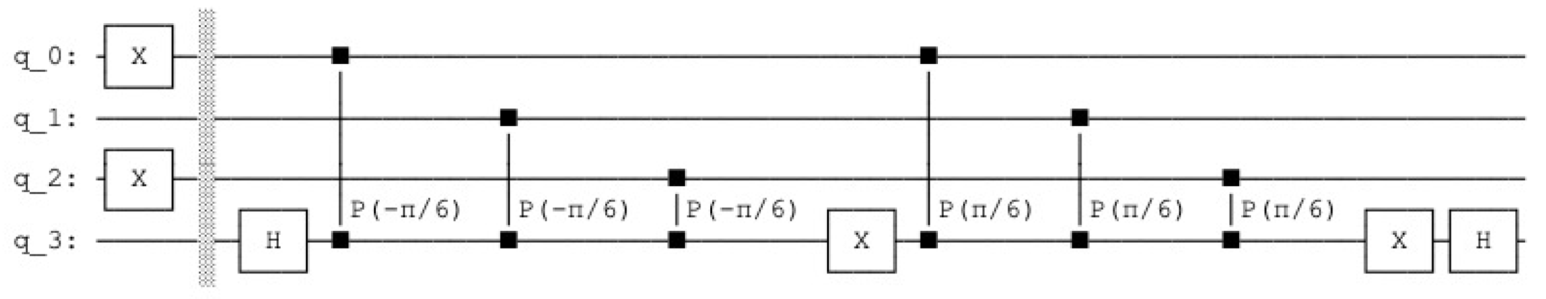
This operation can be implemented by quantum counting of ones. In our example, the state is represented by qubits, of which two () are one.
To count the number of ones, we introduced the control qubit in superposition . For the superposition part represented by the control qubit 0, the phase is applied for each one. For the superposition part represented by the control qubit 1, the phase is applied for each one.
If we apply a Hadamard gate to the control qubit [4], we obtain
The probability of measuring the control qubit is
and the probability of measuring the control qubit is
indicating the presence of two ones. The representation of the circuit in qiskit is given by
- from qiskit import QuantumCircuit, Aer, execute
- from qiskit.visualization import plot_histogram
- from math import~pi
- qc = QuantumCircuit(4)
- #Input is |101>
- qc.x(0)
- qc.x(2)
- qc.barrier()
- qc.h(3)
- qc.cp(-pi/6,0,3)
- qc.cp(-pi/6,1,3)
- qc.cp(-pi/6,2,3)
- qc.x(3)
- qc.cp(pi/6,0,3)
- qc.cp(pi/6,1,3)
- qc.cp(pi/6,2,3)
- qc.x(3)
- qc.h(3)
- simulator = Aer.get_backend(’statevector_simulator’)
- # Run and get counts
- result=execute(qc,simulator).result()
- counts = result.get_counts()
- plot_histogram(counts)
6. Quantum Lernmatrix
Useful associative properties result from equally distributed weights over the whole weight matrix and are only present in large matrices, in our examples we examine toys examples as a proof of concept for future quantum associative memories.
The superposition of the weight vectors of the units is based on the entanglement of the index qubits that are in the superposition with the weight vectors. The count is represented by a unary string of qubits that controls the phase operation. It represents the value of the Lernmatrix. The phase information is the basis of the quantum counting of ones that increases the probability of measuring the correct units representing ones in the answer vector. We will represent n units in superposition by entanglement with the index qubits.
To represent four 4 units, we need two index qubits in superposition. Each index state of the qubit is entangled with a pattern by the Toffoli gate also called the ccX gate (CCNOT gate, controlled controlled not gate), by setting a corresponding qubit to one. In our example, we store three patterns ; , ; and ; resulting in the weight matrix represented by four units (see Figure 9).
After the entanglement of index qubits in superposition
with the weight vectors the following state is present, the state and are represented by four qubits each for the four binary weights, with
(see Figure 10)
With
The value is the unary representation of the Lernmatrix value . We include the query vector as ,
the resulting histogram of the measured qubits is represented in Figure 11.
In the next step, we describe the active phase (see Figure 12).
For simplicity, we will ignore the index qubits, since they are not important in the active phase. We perform quantum counting using the control bit that is set in superposition resulting in
Applying controlled phase operation with since two ones are present in the query vector and
and applying the Hadamard gate to the control qubit, we obtain
The architecture is described by fifteen qubits, see Appendix A. With the query vector units represented by the states have following values:
- The first unit has the value and the two corresponding states are: for the control the value is with the measured probability and for the control the value is with the measured probability 0.
- The second unit has the value and the two corresponding states are: for the control the value is with the measured probability and for the control the value is with the measured probability .
- The third unit has the value and the two corresponding states are: for the control the value is with the measured probability = 0 and for the control the value is with the measured probability = 0.
- The fourth unit has the (decimal) value and the two corresponding states are: for the control the value is with the measured probability and for the control the value is with the measured probability 0.
There are five states with probabilities not equal to zero, see Figure 13. The measured probability (control ) indicating a firing of the units is .
6.1. Generalization
We can generalize the description for n units. After the entanglement of index qubits in superposition with the weight vectors, the following state is present, and the state and are represented by [4,5],
with the cost . We apply the control qubit (ignoring the index qubits)
Applying controlled phase operation with N for present ones in the query vector and
and applying the Hadamard gate to the control qubit, we obtain the final result with
The cost of one query is and for queries .
6.2. Example
In this example, we store three patterns representing three associations: ; , ; and ; . The weight matrix after the learning phase is represented by eight units (see Figure 14 and Figure 15).
After the entanglement of index qubits in superposition
with the weight vectors, the following state is present, the state and are represented by eight qubits [4,5],
With the query vector as , we obtain (see Figure 16)
and the answer vector (ignoring the index qubits) according to
is (see Figure 17).
7. Applying Trugenberger Amplification Several Times
According to Trugenberger [5], applying the control qubit sequential b times results in
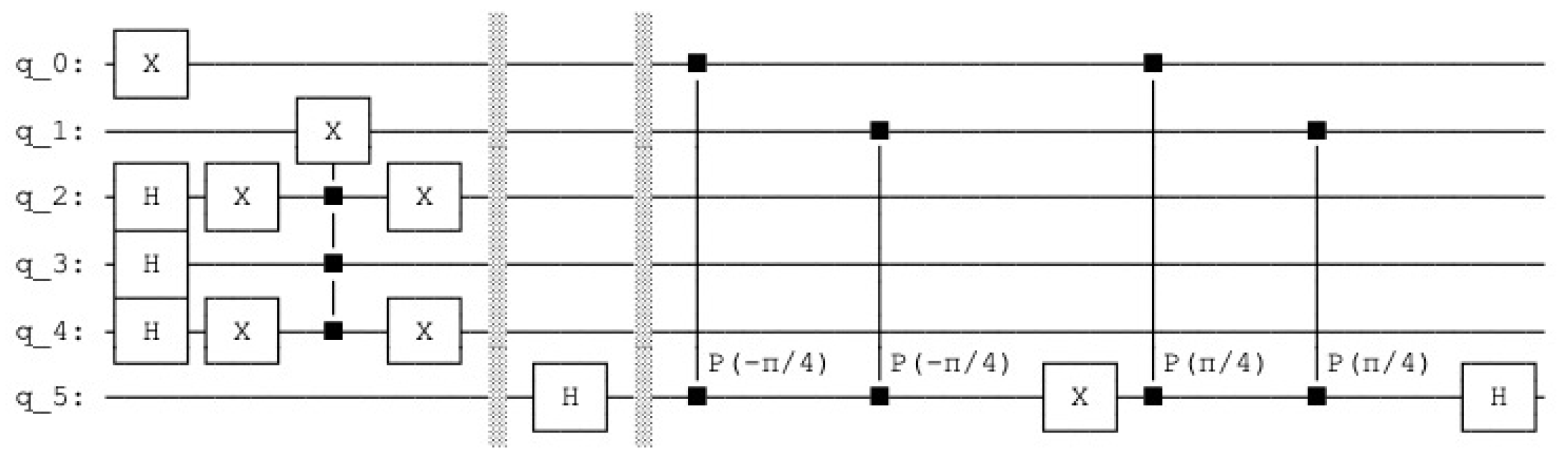
with being the binary representation of the decimal value v. The idea is then to measure b control qubits b times, until the desired state is obtained. Trugenberger identifies the inverse parameter b as temperature and concludes that the accuracy of pattern recall can be tuned by adjusting a parameter playing the role of an effective temperature [5]. In Figure 18, the control qubit was applied two times for the quantum circuit of the Figure 10. Figure 19 represents the resulting histogram of the measured qubits.
Relation to b
Trugenberger [5] identifies as a temperature and concludes: the lower t; the better one can identify the desired states. Assuming we have eight states indicated by the index qubit 2, 3 and 4, one marked state 010 has the count two, and the other seven state the count of one, see Figure 20. Figure 21 represents the resulting histogram of the measured qubits and Figure 22 represents the resulting histogram after applying the control qubit two times .
Now we can take the idea further and generalize it. For n states, one state is marked with the count of 2, and all other remaining states have the count of 1. Since there are n states, the marked state has the probability value and the remaining states have the probability value . It follows
and
For the next control qubit, we would obtain
with
resulting in the sequence
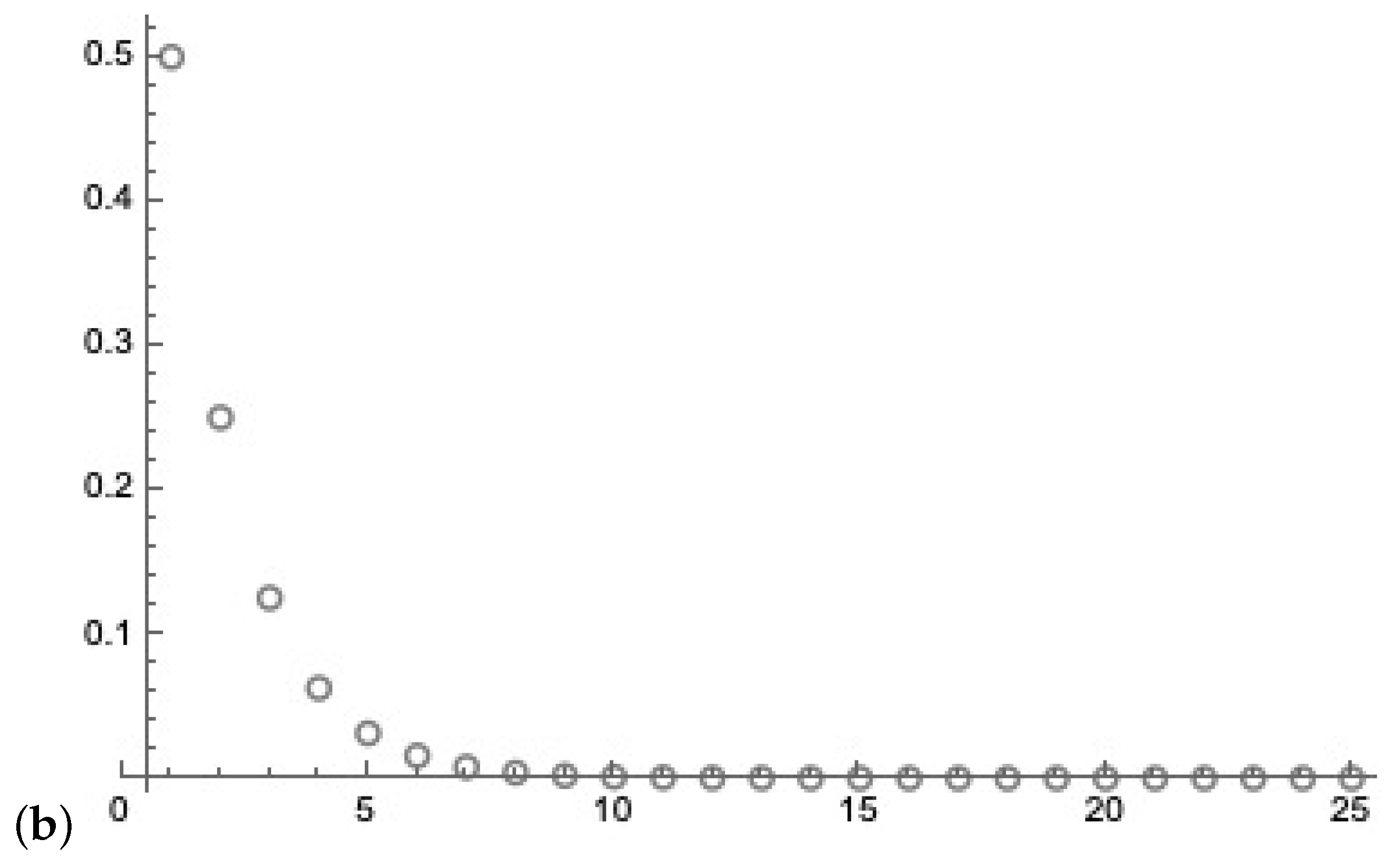
After measuring the control qubit at step b, the probability of the marked state is (see Figure 23)
and with the probability of measuring the control qubit at step b
With the assumption of independence, measuring the control qubits in the sequence
results in a low probability (see Figure 23). The assumption that “if t is lower (higher b;) than the determination of the desired states is better” is not correct. As a consequence, we can measure the sequential control qubits two times before the task becomes not tractable.
8. Tree-like Structures
We want to increase the probability of measuring the correct units representing the ones in the answer vector and decrease the probability of measuring the zeros. For example, in a sparse code with k ones, k measurements of different ones reconstruct the binary answer vector and we cannot use the idea of applying Trugenberger amplification several times as indicated before. Instead, we can increase the probability of measuring a one by the introduced tree-like structure [44]. The tree-like hierarchical associative memory approach is based on aggregation of the neighboring units [44]. The aggregation is a Boolean OR-based transform for two or three neighboring weights of unit results resulting in a more dense memory, see Figure 24.
It was shown by computer experiments that the aggregation value between two and three is an optimal one [45]. The more dense memory is copied on top or the original memory. Depending on the number of units, we can repeat the process in which we aggregate groups of two to three neighboring groups of equal units. We can continue the process till we arrive in two different groups of different units, the number of possible different aggregated memories is logarithmic, with . Since in our example only four units are present, we aggregate two units resulting in a memory of four units described by 2 identical units each.
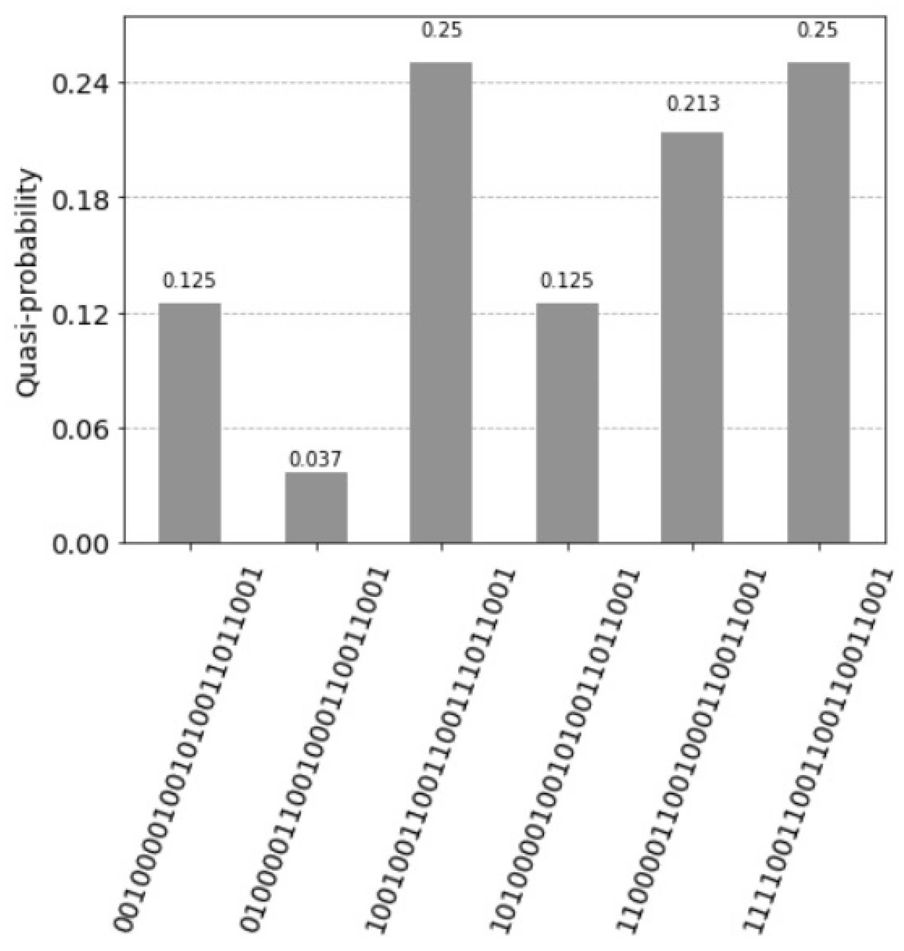
The query vector is composed of concatenated copies of the original query vector, in our example . We apply controlled phase operation with with , see Figure 24 and Appendix B. The measured probability (control ) indicating a firing of the units is and there are six states not equal to zero, see Figure 25 and compare with Figure 11.
9. Costs
We cannot clone an arbitrary quantum state; however, it was proposed that a quantum state can be probabilistic cloned up to a mirror modular transformation [14]. In an alternative approach, we prepare a set of quantum Lernmatrices in superposition. This preparation requires a great deal of time and we name it the sleep phase. The cost of storing patterns in n units with in a Lernmatrix and consequently the quantum Lernmatrix is [18,19]. On the other hand, in the active phase, the query operation is extremely fast.
Query Cost of Quantum Lernmatrix
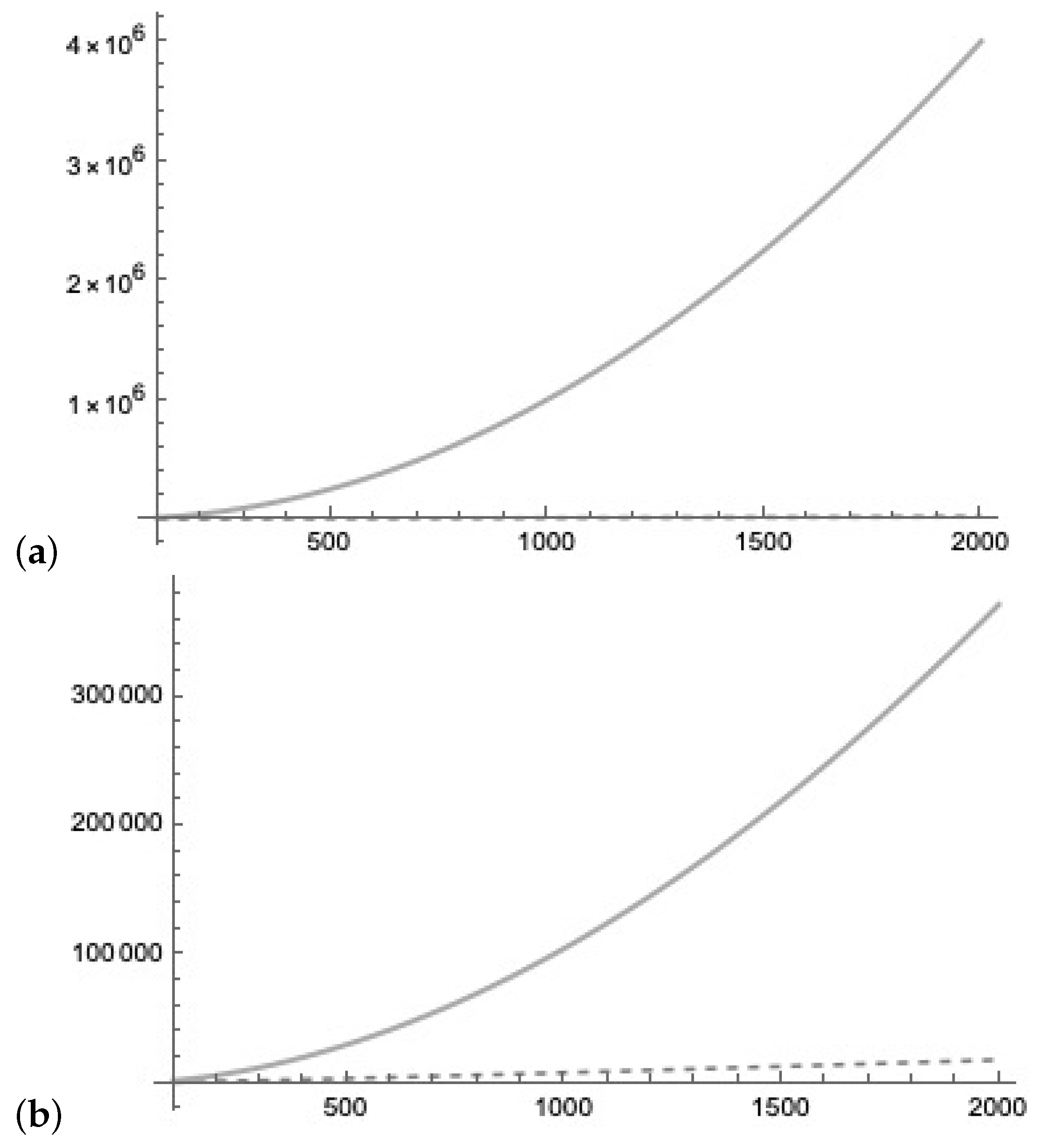
During the active phase, the quantum Lernmatrices are sampled with minimal costs in time. In Figure 26a, we compare the query cost of k queries of the quantum Lernmatrix representing the weight matrix of the size to the cost of a classical Lernmatrix of the size , which are
In Figure 26b, we compare the query cost of k queries of the quantum Lernmatrix representing the weight matrix of the size to Grover’s amplification algorithm on a list of L vectors of dimension n
10. Conclusions
We introduced a quantum Lernmatrix based on the Monte Carlo Lernmatrix and preformed experiments using qiskit as a proof of concept for future quantum associative memories. We proposed a tree-like structure that increases the measured value for the control qubit indicating a firing of the units. Our approach does not solve the input destruction problem but gives a hint how to deal with it. We represent the preparation costs and the query time by two phases.
The cost of the sleep phase and the active phase are the same as one of a conventional associative memory . We assume that in the sleep phase we have enough time to prepare several quantum Lernmatrices in superposition. The quantum Lernmatrices are kept in superposition until they are queried in the active phase. Each of the copies of the quantum Lernmatrix can be queried only once. We argue that the advantage to conventional associative memories is present in the active phase were the fast determination of information is essential by the use of quantum Lernmatrices in superposition compared to the cost of the classical Lernmatrix .
Funding
This work was supported by national funds through FCT, Fundação para a Ciência e a Tecnologia, under project UIDB/50021/2020. The funders had no role in study design, data collection and analysis, decision to publish, or preparation of the manuscript. The authors declare no conflicts of interest. This article does not contain any studies with human participants or animals performed by any of the authors.
Data Availability Statement
Not appliable.
Acknowledgments
The author acknowledges the use of IBM Quantum services for this work. The views expressed are those of the author, and do not reflect the official policy or position of IBM or the IBM Quantum team.
Conflicts of Interest
The author declares no conflict of interest.
Appendix A. Quantum Lernmatrix
In our architecture the qubits 0 to 3 represent the query vector, the qubits 4 to 7 the associative memory, the qubits 8 to 11 represent the count and the qubits 12 and 13 are the index qubits, the qubit 14 is the control qubit. The count operation is done by the ccX gate (see Figure 10 and Figure 12)
- qc = QuantumCircuit(15)
- #0-3 query
- #4-7 data
- #8-11 count
- #Index Pointer
- #12-13
- #Aux
- #14
- #Sleep Phase
- #Index Pointer
- qc.h(12)
- qc.h(13)
- qc.barrier()
- #1st weights
- qc.ccx(12,13,4)
- qc.ccx(12,13,7)
- qc.barrier()
- #2th weights
- qc.x(12)
- qc.ccx(12,13,4)
- qc.x(12)
- qc.barrier()
- #3th weights
- qc.x(13)
- qc.ccx(12,13,6)
- qc.x(13)
- qc.barrier()
- #4th weights
- qc.x(12)
- qc.x(13)
- qc.ccx(12,13,4)
- qc.ccx(12,13,7)
- qc.x(13)
- qc.x(12)
- qc.barrier()
- #Active Phase
- #query
- qc.x(0)
- qc.x(3)
- qc.barrier()
- qc.ccx(0,4,8)
- qc.ccx(1,5,9)
- qc.ccx(2,6,10)
- qc.ccx(3,7,11)
- #Dividing
- qc.h(14)
- qc.barrier()
- #Marking
- qc.cp(-pi/4,8,14)
- qc.cp(-pi/4,9,14)
- qc.cp(-pi/4,10,14)
- qc.cp(-pi/4,11,14)
- qc.barrier()
- qc.x(14)
- qc.cp(pi/4,8,14)
- qc.cp(pi/4,9,14)
- qc.cp(pi/4,10,14)
- qc.cp(pi/4,11,14)
- qc.h(14)
- qc.draw(fold=110)
Appendix B. Quantum Tree-like Lernmatrix
- qc = QuantumCircuit(23)
- #0-3 query
- #4-7 data aggregated
- #8-11 data
- #12-19 count
- #Index Pointer
- #20-21
- #Aux
- #22
- #Sleep Phase
- #Index Pointer
- qc.h(20)
- qc.h(21)
- #1st weights
- #OR Aggregated
- qc.barrier()
- qc.ccx(20,21,4)
- qc.ccx(20,21,7)
- #Original
- qc.barrier()
- qc.ccx(20,21,8)
- qc.ccx(20,21,11)
- #2th weights
- qc.x(20)
- #OR Aggregated
- qc.barrier()
- qc.ccx(20,21,4)
- qc.ccx(20,21,7)
- #Original
- qc.barrier()
- qc.ccx(20,21,8)
- qc.x(20)
- #3th weights
- qc.x(21)
- #OR Aggregated
- qc.barrier()
- qc.ccx(20,21,4)
- qc.ccx(20,21,6)
- qc.ccx(20,21,7)
- #Original
- qc.barrier()
- qc.ccx(20,21,10)
- qc.x(21)
- #4th weights
- qc.x(20)
- qc.x(21)
- #OR Aggregated
- qc.barrier()
- qc.ccx(20,21,4)
- qc.ccx(20,21,6)
- qc.ccx(20,21,7)
- #Original
- qc.barrier()
- qc.ccx(20,21,8)
- qc.ccx(20,21,11)
- qc.x(21)
- qc.x(20)
- #Active Phase
- #query
- qc.barrier()
- qc.x(0)
- qc.x(3)
- qc.barrier()
- #query, counting
- #OR Aggregated
- qc.ccx(0,4,12)
- qc.ccx(1,5,13)
- qc.ccx(2,6,14)
- qc.ccx(3,7,15)
- #Original
- qc.ccx(0,8,16)
- qc.ccx(1,9,17)
- qc.ccx(2,10,18)
- qc.ccx(3,11,19)
- #Dividing
- qc.barrier()
- qc.h(22)
- #Marking
- qc.barrier()
- qc.cp(-pi/8,12,22)
- qc.cp(-pi/8,13,22)
- qc.cp(-pi/8,14,22)
- qc.cp(-pi/8,15,22)
- qc.cp(-pi/8,16,22)
- qc.cp(-pi/8,17,22)
- qc.cp(-pi/8,18,22)
- qc.cp(-pi/8,19,22)
- qc.barrier()
- qc.x(22)
- qc.cp(pi/8,12,22)
- qc.cp(pi/8,13,22)
- qc.cp(pi/8,14,22)
- qc.cp(pi/8,15,22)
- qc.cp(pi/8,16,22)
- qc.cp(pi/8,17,22)
- qc.cp(pi/8,18,22)
- qc.cp(pi/8,19,22)
- qc.barrier()
- qc.h(22)
- qc.draw()
References
- Ventura, D.; Martinez, T. Quantum associative memory with exponential capacity. In Proceedings of the 1998 IEEE International Joint Conference on Neural Networks Proceedings. IEEE World Congress on Computational Intelligence, Anchorage, AK, USA, 4–9 May 1988; Volume 1, pp. 509–513. [Google Scholar]
- Ventura, D.; Martinez, T. Quantum associative memory. Inf. Sci. 2000, 124, 273–296. [Google Scholar] [CrossRef]
- Tay, N.; Loo, C.; Perus, M. Face Recognition with Quantum Associative Networks Using Overcomplete Gabor Wavelet. Cogn. Comput. 2010, 2, 297–302. [Google Scholar] [CrossRef]
- Trugenberger, C.A. Probabilistic Quantum Memories. Phys. Rev. Lett. 2001, 87, 067901. [Google Scholar] [CrossRef] [PubMed]
- Trugenberger, C.A. Quantum Pattern Recognition. Quantum Inf. Process. 2003, 1, 471–493. [Google Scholar] [CrossRef]
- Schuld, M.; Petruccione, F. Supervised Learning with Quantum Computers; Springer: Berlin/Heidelberg, Germany, 2018. [Google Scholar]
- Grover, L.K. A fast quantum mechanical algorithm for database search. In Proceedings of the STOC’96: Proceedings of the Twenty-Eighth Annual ACM Symposium on Theory of Computing, Philadelphia, PA, USA, 22–24 May 1996; ACM: New York, NY, USA, 1996; pp. 212–219. [Google Scholar] [CrossRef]
- Grover, L.K. Quantum Mechanics helps in searching for a needle in a haystack. Phys. Rev. Lett. 1997, 79, 325. [Google Scholar] [CrossRef]
- Grover, L.K. A framework for fast quantum mechanical algorithms. In Proceedings of the STOC’98: Proceedings of the Thirtieth Annual ACM Symposium on Theory of Computing, Dallas, TX, USA, 24–26 May 1998; ACM: New York, NY, USA, 1998; pp. 53–62. [Google Scholar] [CrossRef]
- Grover, L.K. Quantum Computers Can Search Rapidly by Using Almost Any Transformation. Phys. Rev. Lett. 1998, 80, 4329–4332. [Google Scholar] [CrossRef]
- Aïmeur, E.; Brassard, B.; Gambs, S. Quantum speed-up for unsupervised learning. Mach. Learn. 2013, 90, 261–287. [Google Scholar] [CrossRef]
- Wittek, P. Quantum Machine Learning, What Quantum Computing Means to Data Mining; Elsevier Insights; Academic Press: Cambridge, MA, USA, 2014. [Google Scholar]
- Aaronson, S. Quantum Machine Learning Algorithms: Read the Fine Print. Nat. Phys. 2015, 11, 291–293. [Google Scholar] [CrossRef]
- Diamantini, M.C.; Trugenberger, C.A. Mirror modular cloning and fast quantum associative retrieval. arXiv 2022, arXiv:2206.01644. [Google Scholar]
- Brun, T.; Klauck, H.; Nayak, A.; Rotteler, M.; Zalka, C. Comment on “Probabilistic Quantum Memories”. Phys. Rev. Lett. 2003, 91, 209801. [Google Scholar] [CrossRef] [PubMed]
- Harrow, A.; Hassidim, A.; Lloyd, S. Quantum algorithm for solving linear systems of equations. Phys. Rev. Lett. 2009, 103, 150502. [Google Scholar] [CrossRef]
- Schuld, M.; Killoran, N. Quantum Machine Learning in Feature Hilbert Spaces. Phys. Rev. Lett. 2019, 122, 040504. [Google Scholar] [CrossRef]
- Palm, G. Neural Assemblies, an Alternative Approach to Artificial Intelligence; Springer: Berlin/Heidelberg, Germany, 1982. [Google Scholar]
- Hecht-Nielsen, R. Neurocomputing; Addison-Wesley: Reading, PA, USA, 1989. [Google Scholar]
- Steinbuch, K. Die Lernmatrix. Kybernetik 1961, 1, 36–45. [Google Scholar] [CrossRef]
- Steinbuch, K. Automat und Mensch, 4th ed.; Springer: Berlin/Heidelberg, Germany, 1971. [Google Scholar]
- Willshaw, D.; Buneman, O.; Longuet-Higgins, H. Nonholgraphic associative memory. Nature 1969, 222, 960–962. [Google Scholar] [CrossRef] [PubMed]
- Contributors, Q. Qiskit: An Open-source Framework for Quantum Computing. Zenodo 2023. [Google Scholar] [CrossRef]
- Palm, G. Assoziatives Gedächtnis und Gehirntheorie. In Gehirn und Kognition; Spektrum der Wissenschaft: Heidelberg, Germany, 1990; pp. 164–174. [Google Scholar]
- Churchland, P.S.; Sejnowski, T.J. The Computational Brain; The MIT Press: Cambridge, MA, USA, 1994. [Google Scholar]
- Fuster, J. Memory in the Cerebral Cortex; The MIT Press: Cambridge, MA, USA, 1995. [Google Scholar]
- Squire, L.R.; Kandel, E.R. Memory: From Mind to Moleculus; Scientific American Library: New York, NY, USA, 1999. [Google Scholar]
- Kohonen, T. Self-Organization and Associative Memory, 3rd ed.; Springer: Berlin/Heidelberg, Germany, 1989. [Google Scholar]
- Hertz, J.; Krogh, A.; Palmer, R.G. Introduction to the Theory of Neural Computation; Addison-Wesley: Reading, PA, USA, 1991. [Google Scholar]
- Anderson, J.R. Cognitive Psychology and Its Implications, 4th ed.; W. H. Freeman and Company: New York, NY, USA, 1995. [Google Scholar]
- Amari, S. Learning Patterns and Pattern Sequences by Self-Organizing Nets of Threshold Elements. IEEE Trans. Comput. 1972, 100, 1197–1206. [Google Scholar] [CrossRef]
- Anderson, J.A. An Introduction to Neural Networks; The MIT Press: Cambridge, MA, USA, 1995. [Google Scholar]
- Ballard, D.H. An Introduction to Natural Computation; The MIT Press: Cambridge, MA, USA, 1997. [Google Scholar]
- Hopfield, J.J. Neural networks and physical systems with emergent collective computational abilities. Proc. Natl. Acad. Sci. USA 1982, 79, 2554–2558. [Google Scholar] [CrossRef] [PubMed]
- McClelland, J.; Kawamoto, A. Mechanisms of Sentence Processing: Assigning Roles to Constituents of Sentences. In Parallel Distributed Processing; McClelland, J., Rumelhart, D., Eds.; The MIT Press: Cambridge, MA, USA, 1986; pp. 272–325. [Google Scholar]
- OFTA. Les Re´seaux de Neurones; Masson: Paris, France, 1991. [Google Scholar]
- Schwenker, F. Küntliche Neuronale Netze: Ein Überblick über die theoretischen Grundlagen. In Finanzmarktanalyse und-Prognose mit Innovativen und Quantitativen Verfahren; Bol, G., Nakhaeizadeh, G., Vollmer, K., Eds.; Physica-Verlag: Heidelberg, Germany, 1996; pp. 1–14. [Google Scholar]
- Sommer, F.T. Theorie Neuronaler Assoziativspeicher. Ph.D. Thesis, Heinrich-Heine-Universität Düsseldorf, Düsseldorf, Germany, 1993. [Google Scholar]
- Wickelgren, W.A. Context-Sensitive Coding, Associative Memory, and Serial Order in (Speech) Behavior. Psychol. Rev. 1969, 76, 1–15. [Google Scholar] [CrossRef]
- Sa-Couto, L.; Wichert, A. “What-Where” sparse distributed invariant representations of visual patterns. Neural Comput. Appl. 2022, 34, 6207–6214. [Google Scholar] [CrossRef]
- Sa-Couto, L.; Wichert, A. Competitive learning to generate sparse representations for associative memory. arXiv 2023, arXiv:2301.02196. [Google Scholar]
- Marcinowski, M. Codierungsprobleme beim Assoziativen Speichern. Master’s Thesis, Fakultät für Physik der Eberhard-Karls-Universität Tübingen, Tübingen, Germany, 1987. [Google Scholar]
- Freeman, J.A. Simulating Neural Networks with Mathematica; Addison-Wesley: Reading, PA, USA, 1994. [Google Scholar]
- Sacramento, J.; Wichert, A. Tree-like hierarchical associative memory structures. Neural Netw. 2011, 24, 143–147. [Google Scholar] [CrossRef] [PubMed]
- Sacramento, J.; Burnay, F.; Wichert, A. Regarding the temporal requirements of a hierarchical Willshaw network. Neural Netw. 2012, 25, 84–93. [Google Scholar] [CrossRef] [PubMed]

Figure 2.
The Lernmatrix is composed of a set of units that represent a simple model of a real biological neuron. The unit is composed of weights, which correspond to the synapses and dendrites in the real neuron. In this Figure, they are described by where and . T is the threshold of the unit.
Figure 2.
The Lernmatrix is composed of a set of units that represent a simple model of a real biological neuron. The unit is composed of weights, which correspond to the synapses and dendrites in the real neuron. In this Figure, they are described by where and . T is the threshold of the unit.

Figure 3.
The vector pair and is learned. The corresponding binary weights of the associated pair are indicated by a black square. In the next step, the vector pair and is learned. The corresponding binary weights of the associated pair are indicated by a black circle.
Figure 3.
The vector pair and is learned. The corresponding binary weights of the associated pair are indicated by a black square. In the next step, the vector pair and is learned. The corresponding binary weights of the associated pair are indicated by a black circle.

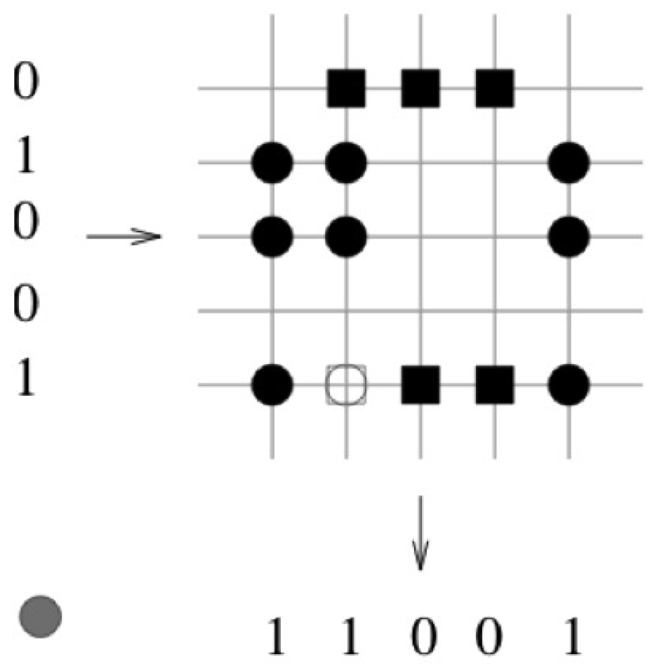
Figure 4.
The query vector differs by one bit to the learned query vector . The threshold T is set to the number of “one” components in the query vector , . The retrieved vector is the vector that was stored.
Figure 4.
The query vector differs by one bit to the learned query vector . The threshold T is set to the number of “one” components in the query vector , . The retrieved vector is the vector that was stored.

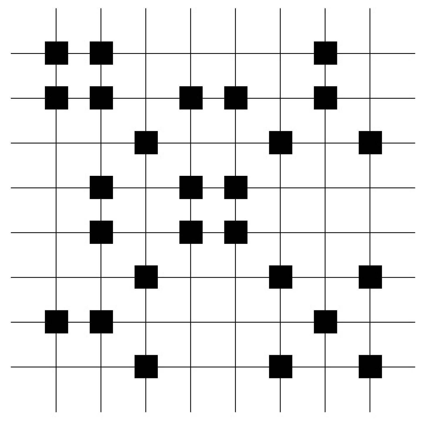
Figure 5.
The weight matrix after learning of 20,000 test patterns, in which ten ones were randomly set in a 2000 dimensional vector represents a high loaded matrix with equally distributed weights. This example shows that the weight matrix diagram often contains nearly no information. Information about the weight matrix can be extracted by the structure of weight matrix. (White color represents wights.)

Figure 6.
Sigmoid-like probability functions for is indicated by continuous line, the linear relation by the dashed lines. The x-axis indicates the k values, and the y-axis the probabilities.
Figure 6.
Sigmoid-like probability functions for is indicated by continuous line, the linear relation by the dashed lines. The x-axis indicates the k values, and the y-axis the probabilities.

Figure 7.
Quantum counting circuit with and .

Figure 8.
and .

Figure 9.
Wight matrix represented by four units after learning the correlation of the three patterns ; , ; and ; . The learning is identical with the learning phase of the Lernmatrix.
Figure 9.
Wight matrix represented by four units after learning the correlation of the three patterns ; , ; and ; . The learning is identical with the learning phase of the Lernmatrix.

Figure 10.
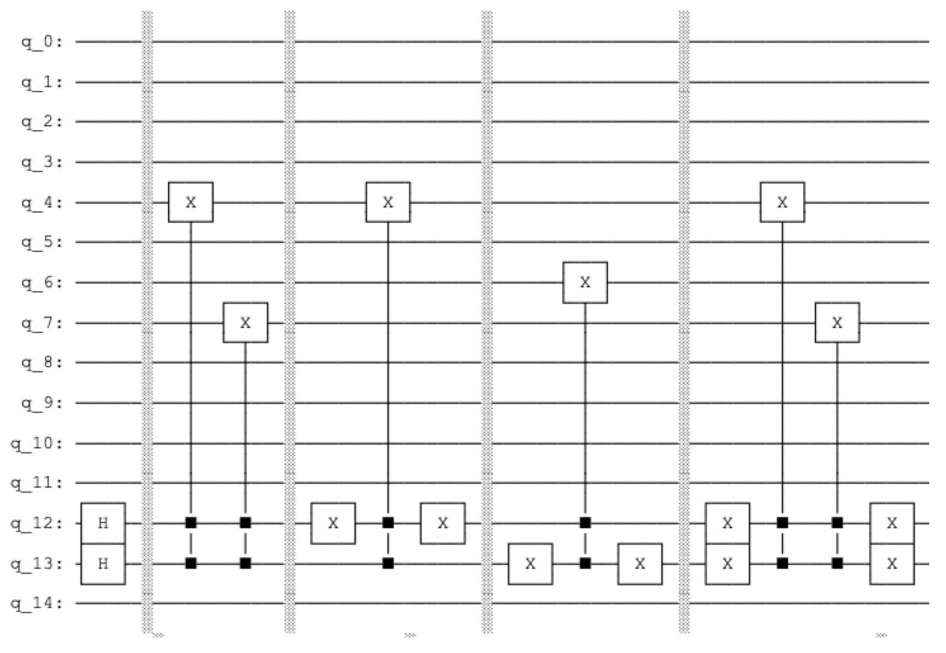
The quantum circuit that produces the sleep phase. The qubits 0 to 3 represent the query vector, the qubits 4 to 7 the associative memory, the qubits 8 to 11 represent the count and the qubits 12 and 13 are the index qubits, while the qubit 14 is the control qubit.
Figure 10.
The quantum circuit that produces the sleep phase. The qubits 0 to 3 represent the query vector, the qubits 4 to 7 the associative memory, the qubits 8 to 11 represent the count and the qubits 12 and 13 are the index qubits, while the qubit 14 is the control qubit.

Figure 11.
Four superposition states corresponding to the four units of the associative memory. The qubits 0 to 3 represent the query vector , the qubits 4 to 7 the associative memory, the qubits 8 to 11 represent the count, the qubits 12 and 13 are the index qubits, and the control qubit 14 is zero. Note that the units are counted in the reverse order by the index qubits: 11 for the first unit, 10 for the third unit, 01 for second unit and 00 for the fourth unit.

Figure 12.
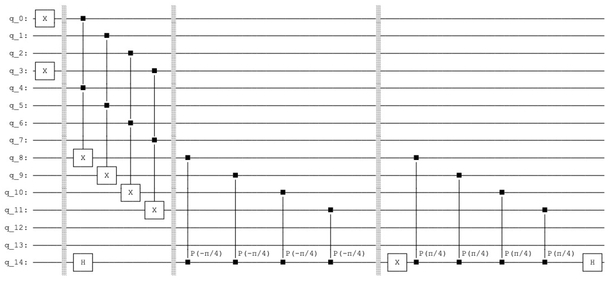
The quantum circuit that produces the active phase. The query and the amplification operations on the count qubits, the qubits 8 to 11. The control qubit 14.
Figure 12.
The quantum circuit that produces the active phase. The query and the amplification operations on the count qubits, the qubits 8 to 11. The control qubit 14.

Figure 13.
Five superposition states not equal to zero. The control qubit 14 equal to one indicates the firing of the units. The measured value is . The two probabilities express the perfect match and the solution , indicated by the index qubits 12 and 13, with the values for the first unit and for the fourth unit. Note that the units are counted in the reverse order by the index qubits: first unit, for the second unit, for third unit and for the fourth unit. The control qubit 14 equal to zero indicates the units that do not fire. The measured value is . The probability with the index qubits 12 and 13, with the value for the third unit indicates the most dissimilar pattern .

Figure 14.
Weight matrix represented by eight units after learning the correlation of the three patterns ; , ; and ; . The learning is identical with the learning phase of the Lernmatrix.
Figure 14.
Weight matrix represented by eight units after learning the correlation of the three patterns ; , ; and ; . The learning is identical with the learning phase of the Lernmatrix.

Figure 15.
The quantum circuit that produces the sleep phase. The qubits 0 to 7 represent the query vector, the qubits 8 to 15 the associative memory, the qubits 16 to 23 represent the count and the qubits 24, 25 and 26 are the index qubits (8 states), and the qubit 27 is the control qubit.
Figure 15.
The quantum circuit that produces the sleep phase. The qubits 0 to 7 represent the query vector, the qubits 8 to 15 the associative memory, the qubits 16 to 23 represent the count and the qubits 24, 25 and 26 are the index qubits (8 states), and the qubit 27 is the control qubit.

Figure 16.
The quantum circuit that produces the active phase. The query and the amplification operations on the count qubits, the qubits 16 to 23 and the control qubit 27.
Figure 16.
The quantum circuit that produces the active phase. The query and the amplification operations on the count qubits, the qubits 16 to 23 and the control qubit 27.

Figure 17.
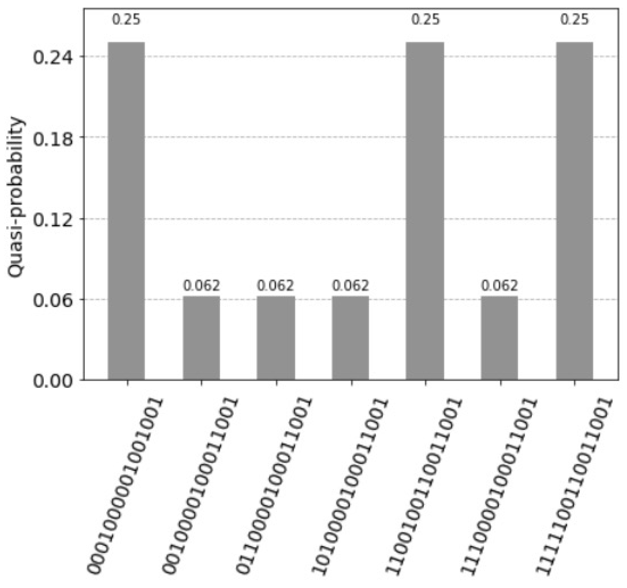
Teen superposition states not equal to zero. The qubits 24, 25 and 26 are the index qubits. Note that the units are counted in the reverse order by the index qubits: 111 first unit, 110 for the second unit, till 000 being the eight unit. The measured value for the control qubit 27 equal to one indicates the firing of the units. The measured value is just . This happens since the weight matrix is relatively small and not homogeneously filled. For the query vector , the three values indicate the answer vector by the index qubits 24, 25 and 26; for the first unit with the value (111), the second unit (110) and seventh unit (001). The control qubit 27 equal to zero indicates the units that do not fire.
Figure 17.
Teen superposition states not equal to zero. The qubits 24, 25 and 26 are the index qubits. Note that the units are counted in the reverse order by the index qubits: 111 first unit, 110 for the second unit, till 000 being the eight unit. The measured value for the control qubit 27 equal to one indicates the firing of the units. The measured value is just . This happens since the weight matrix is relatively small and not homogeneously filled. For the query vector , the three values indicate the answer vector by the index qubits 24, 25 and 26; for the first unit with the value (111), the second unit (110) and seventh unit (001). The control qubit 27 equal to zero indicates the units that do not fire.

Figure 18.
Circuit representing the application of the control qubit two times for the quantum circuit of Figure 10.
Figure 18.
Circuit representing the application of the control qubit two times for the quantum circuit of Figure 10.

Figure 19.
Seven superposition states not equal to zero. This is because the states with the former values were divided into two values by the two control qubits. The first control qubit 15 equal to one indicates the firing of the units. The measured value is . After measuring the first control qubit equal to one, the measured value of the second control qubit 14 equal to one is . Assuming independence, the value of measuring the two control qubits with the value one is . As before, the two values indicate the perfect match and the solution with the values of the index qubits 12 and 13: for the first unit and for the fourth unit.

Figure 20.
Assuming we have eight states indicated by the index qubit 2, 3 and 4, one marked state 010 has the count two, and the other seven state the count of one.
Figure 20.
Assuming we have eight states indicated by the index qubit 2, 3 and 4, one marked state 010 has the count two, and the other seven state the count of one.

Figure 21.
The resulting histogram of the measured qubits of one marked state with the count two, and the other seven state the count of one with applying the control qubit.
Figure 21.
The resulting histogram of the measured qubits of one marked state with the count two, and the other seven state the count of one with applying the control qubit.

Figure 22.
The resulting histogram of the measured qubits of one marked state with the count two, and the other seven state the count of one with applying the control qubit two times.
Figure 22.
The resulting histogram of the measured qubits of one marked state with the count two, and the other seven state the count of one with applying the control qubit two times.

Figure 23.
For , the y-axis indicates the resulting probability. (a) Circles indicate the growth of the probability of the marked state related to the the number of steps of Grover’s amplification indicated by the x-axis. The triangles indicate the growth of the probability of the marked state using Trugenberger amplification with the x-axis indicating the number b of measurements assuming the control qubits are 1. (b) With the assumption of independence, measuring the control qubits in the sequence results in a low probability indicated by the circles. The x-axis indicates the number measurements b of the control qubits. As a consequence, we can measure the sequential control qubits two times before the task becomes not tractable.


Figure 24.
(a) In our example, we store three patterns, , ; , and , , and the query vector is . (b) The aggregation is a Boolean OR-based transform for two neighboring weights of units results resulting in a more dense memory with .
Figure 24.
(a) In our example, we store three patterns, , ; , and , , and the query vector is . (b) The aggregation is a Boolean OR-based transform for two neighboring weights of units results resulting in a more dense memory with .

Figure 25.
Five superposition states not equal to zero. The measured probability (control qubit equal to one) indicates the firing of the units is , the measured probability values are , and .
Figure 25.
Five superposition states not equal to zero. The measured probability (control qubit equal to one) indicates the firing of the units is , the measured probability values are , and .

Figure 26.
(a) We compare the cost of queries to the quantum Lernmatrix (representing the weight matrix of the size ), (dashed line) to the cost of a classical Lernmatrix of the size , . (b) We compare the cost of k queries to the quantum Lernmatrix (representing the weight matrix of the size ), with cost (dashed line) to Grover’s amplification algorithm on a list of L vectors of dimension n with cost .

Disclaimer/Publisher’s Note: The statements, opinions and data contained in all publications are solely those of the individual author(s) and contributor(s) and not of MDPI and/or the editor(s). MDPI and/or the editor(s) disclaim responsibility for any injury to people or property resulting from any ideas, methods, instructions or products referred to in the content. |
© 2023 by the author. Licensee MDPI, Basel, Switzerland. This article is an open access article distributed under the terms and conditions of the Creative Commons Attribution (CC BY) license (https://creativecommons.org/licenses/by/4.0/).
Share and Cite
MDPI and ACS Style
Wichert, A. Quantum Lernmatrix. Entropy 2023, 25, 871. https://doi.org/10.3390/e25060871
AMA Style
Wichert A. Quantum Lernmatrix. Entropy. 2023; 25(6):871. https://doi.org/10.3390/e25060871
Chicago/Turabian StyleWichert, Andreas. 2023. "Quantum Lernmatrix" Entropy 25, no. 6: 871. https://doi.org/10.3390/e25060871
APA StyleWichert, A. (2023). Quantum Lernmatrix. Entropy, 25(6), 871. https://doi.org/10.3390/e25060871
Note that from the first issue of 2016, this journal uses article numbers instead of page numbers. See further details here.