
The Strongly Asynchronous Massive Access Channel

Abstract
1. Introduction
1.1. Past Work
1.2. Contribution
- We propose a new achievability scheme that supports strictly positive values of for identical channels for the users.
- We define a new massive identification paradigm in which we allow the number of sequences in a classical identification problem to increase exponentially with the sequence blocklength (or sample size). We find asymptotically matching upper and lower bounds on the probability of identification error for this problem. We use this result in our SAS-DM-MAC model to recover the identity of the users.
- We propose a new achievability scheme for the case that the channels are chosen from a set of conditional distributions. The size of the set increases polynomially in the blocklength n. In this case, the channel statistics themselves can be used for user identification.
- We propose a new achievability scheme without imposing any restrictive assumptions on the users’ channels. We show that strictly positive are possible.
- We propose a novel converse bound for the capacity of the SAS-DM-MAC.
- We show that for , not even reliable synchronization is possible.
1.3. Paper Organization
2. Notations and Problem Formulation
2.1. Notation
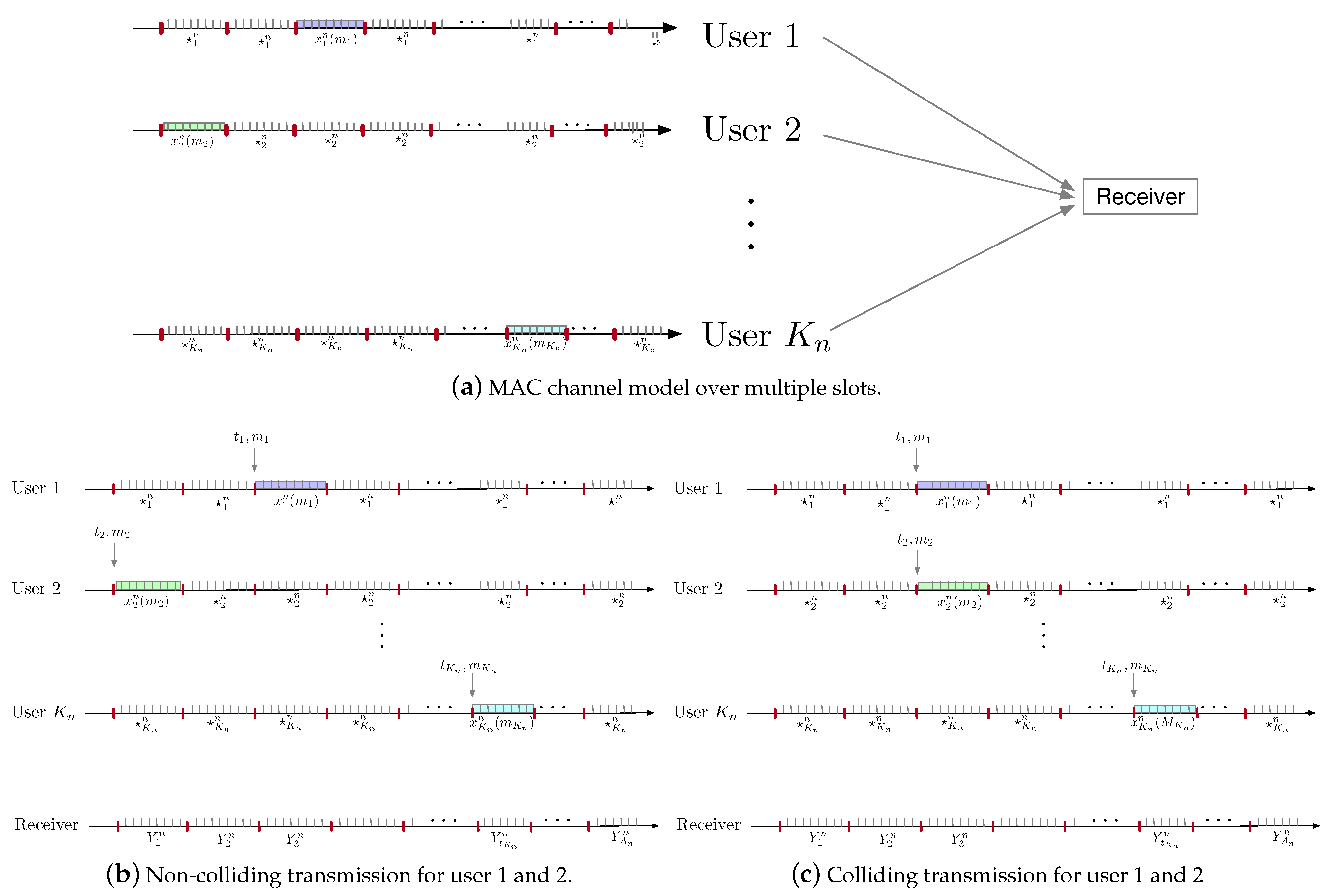
2.2. SAS-DM-MAC Problem Formulation
- A message set , for each user .
- An encoding function , for each user . We define
- Each user chooses a message and a block index (called ‘active’ block henceforth), both uniformly at random. It then transmits , where is the designated idle symbol for user i.
- A destination decoding functionsuch that its associated probability of error, , satisfies wherewhere the hypothesis that user has chosen to transmit message in block is denoted by .
2.3. Identification Problem Formulation
3. Main Results
3.1. Users with Identical Channels
3.2. Users with Different Choice of Channels
3.3. General Case
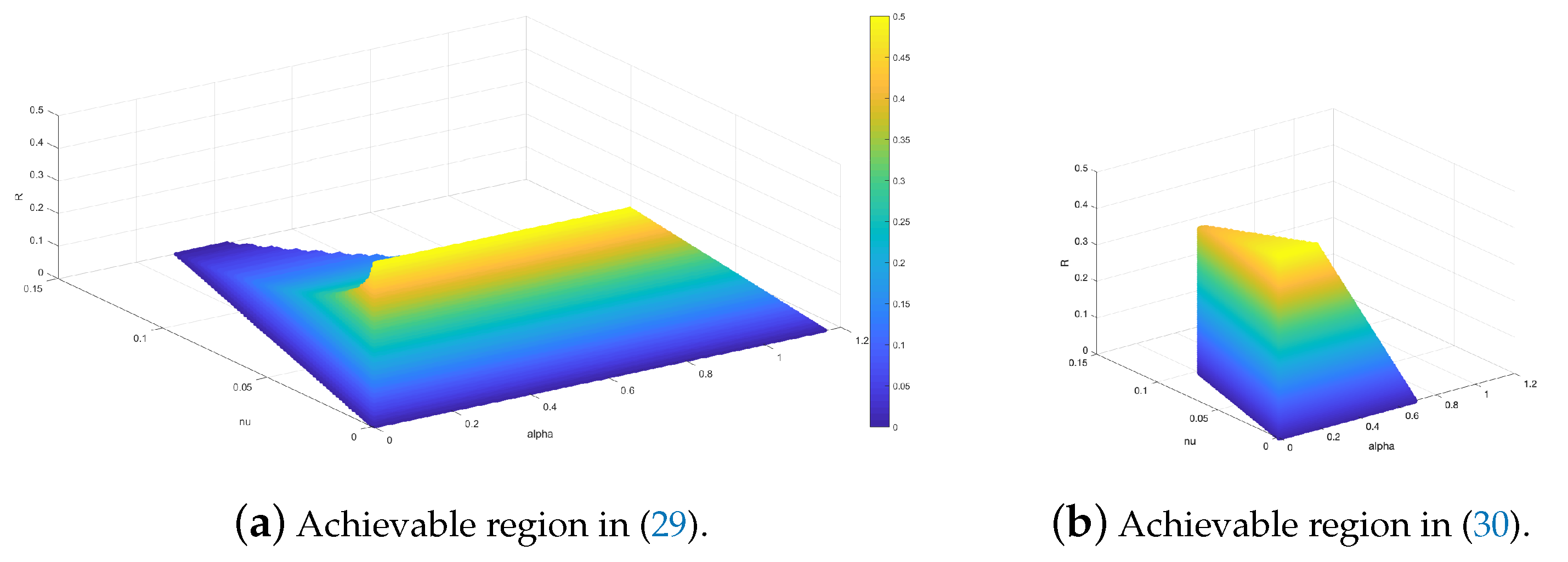
3.4. Example
3.5. Converse on the Capacity Region of the SAS-DM-MAC
3.6. Converse on the Number of Users in a SAS-DM-MAC
4. Discussion and Conclusions
Author Contributions
Funding
Institutional Review Board Statement
Data Availability Statement
Conflicts of Interest
Appendix A. Proof of Theorem 1
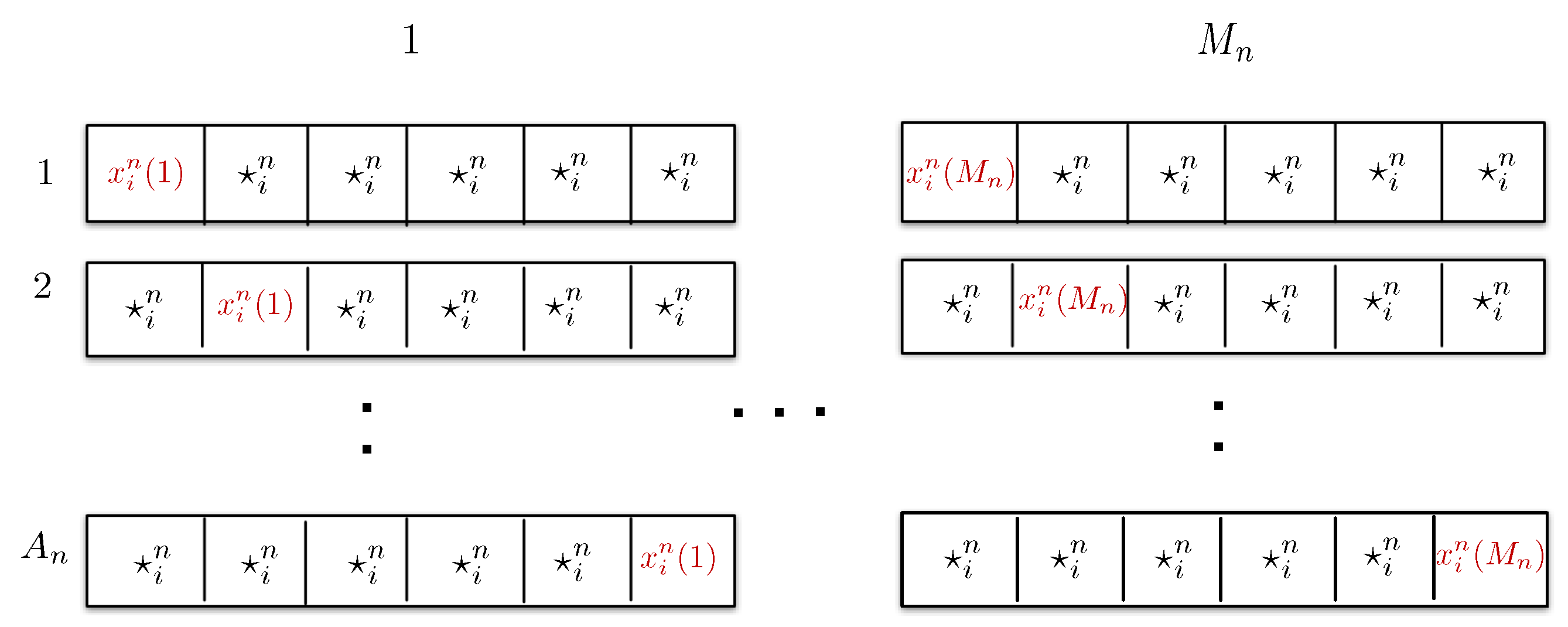
Appendix A.1. Codebook Generation
Appendix A.2. The Decoder and Analysis of the Probability of Error
Appendix B. Proof of Theorem 2
Appendix B.1. Upper Bound on the Probability of Identification Error


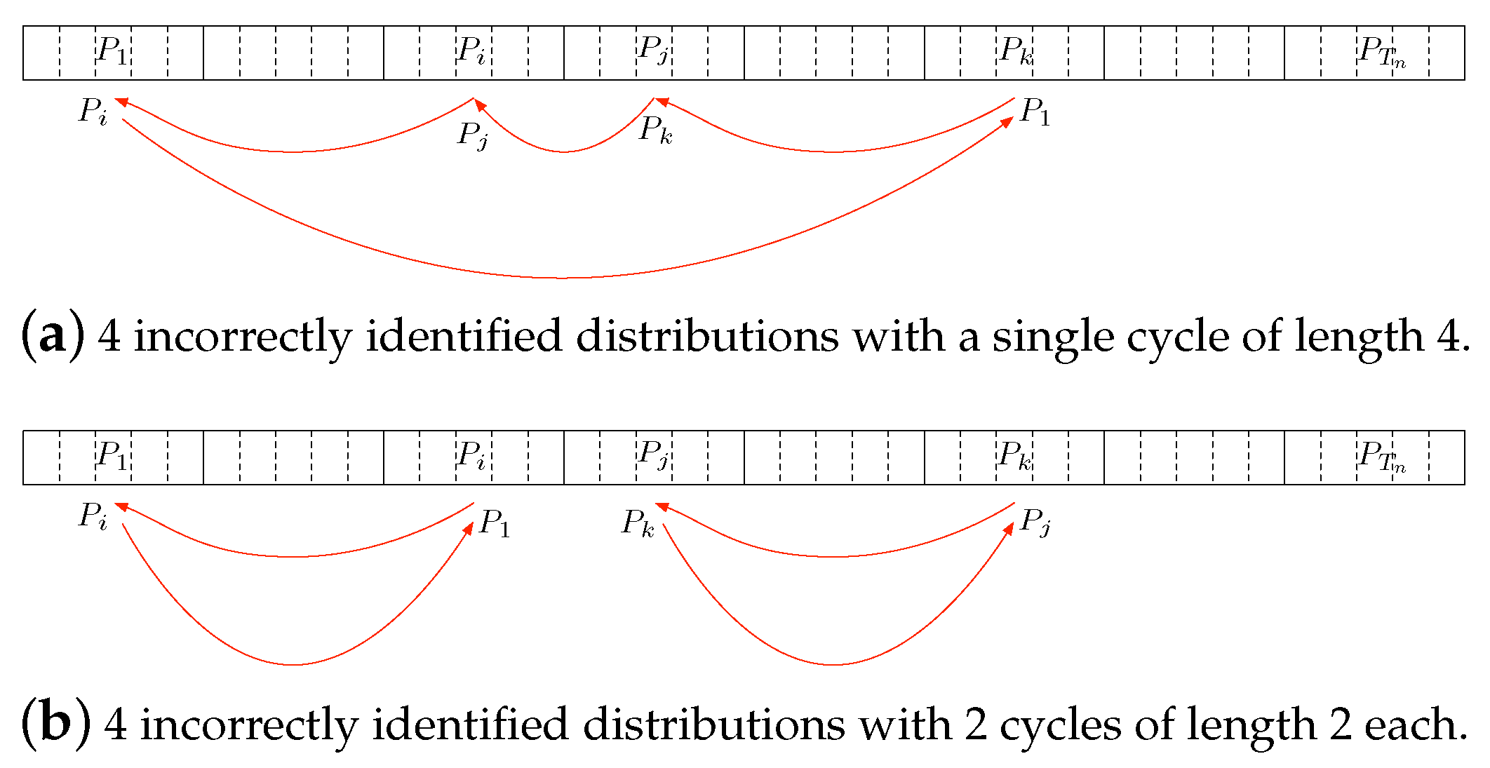
Appendix B.2. Lower Bound on the Probability of Identifiability Error
Appendix C. Proof of Lemma A1

Grouping Scheme
Appendix D. Proof of (A9)
Appendix E. Proof of (A13a)
Appendix F. Proof of Theorem 3
Appendix F.1. Codebook Generation
Appendix F.2. Probability of Error Analysis
Appendix G. Proof of Theorem 4
Appendix H. Proof of (28)
Appendix I. Proof of Theorem 5
Appendix J. Proof of Theorem 6

Appendix K. Proof of (A33a) and (A33b)
Appendix L. Proof of Lemma 1
References
- Chandar, V.; Tchamkerten, A.; Wornell, G. Optimal Sequential Frame Synchronization. IEEE Trans. Inf. Theory 2008, 54, 3725–3728. [Google Scholar] [CrossRef]
- Tchamkerten, A.; Chandar, V.; Wornell, G.W. Asynchronous Communication: Capacity Bounds and Suboptimality of Training. IEEE Trans. Inf. Theory 2013, 59, 1227–1255. [Google Scholar] [CrossRef]
- Tchamkerten, A.; Chandar, V.; Caire, G. Energy and Sampling Constrained Asynchronous Communication. IEEE Trans. Inf. Theory 2014, 60, 7686–7697. [Google Scholar] [CrossRef]
- Chen, X.; Chen, T.Y.; Guo, D. Capacity of Gaussian many-access channels. IEEE Trans. Inf. Theory 2017, 63, 3516–3539. [Google Scholar] [CrossRef]
- Polyanskiy, Y. A perspective on massive random-access. In Proceedings of the IEEE International Symposium on Information Theory (ISIT), Aachen, Germany, 25–30 June 2017; pp. 2523–2527. [Google Scholar] [CrossRef]
- Ahlswede, R.; Dueck, G. Identification via channels. IEEE Trans. Inf. Theory 1989, 35, 15–29. [Google Scholar] [CrossRef]
- Han, T.S.; Verdu, S. Identification Plus Transmission. In Proceedings of the 1991 IEEE International Symposium on Information Theory, Budapest, Hungary, 24–28 June 1991; p. 267. [Google Scholar] [CrossRef]
- Kiefer, J.; Sobel, M. Sequential Identification and Ranking Procedures, with Special Reference to Koopman-Darmois Populations; University of Chicago Press: Chicago, IL, USA, 1968. [Google Scholar]
- Ahlswede, R.; Haroutunian, E. On logarithmically asymptotically optimal testing of hypotheses and identification. In General Theory of Information Transfer and Combinatorics; Springer: Berlin/Heidelberg, Germany, 2006; pp. 553–571. [Google Scholar]
- Unnikrishnan, J. Asymptotically optimal matching of multiple sequences to source distributions and training sequences. IEEE Trans. Inf. Theory 2015, 61, 452–468. [Google Scholar] [CrossRef]
- Shahi, S.; Tuninetti, D.; Devroye, N. On the capacity of strong asynchronous multiple access channels with a large number of users. In Proceedings of the IEEE International Symposium on Information Theory (ISIT), Barcelona, Spain, 10–15 July 2016; pp. 1486–1490. [Google Scholar] [CrossRef]
- Shahi, S.; Tuninetti, D.; Devroye, N. On the capacity of the slotted strongly asynchronous channel with a bursty user. In Proceedings of the 2017 IEEE Information Theory Workshop (ITW), Kaohsiung, Taiwan, 6–10 November 2017; pp. 91–95. [Google Scholar] [CrossRef][Green Version]
- Shahi, S.; Tuninetti, D.; Devroye, N. On Identifying a Massive Number of Distributions. In Proceedings of the IEEE International Symposium on Information Theory (ISIT), Vail, CO, USA, 17–22 June 2018. [Google Scholar]
- Gallager, R.G. Information Theory and Reliable Communication; Springer: Berlin/Heidelberg, Germany, 1968; Volume 588. [Google Scholar]
- Polyanskiy, Y. Asynchronous Communication: Exact Synchronization, Universality, and Dispersion. IEEE Trans. Inf. Theory 2013, 59, 1256–1270. [Google Scholar] [CrossRef][Green Version]
- Chandar, V.; Tchamkerten, A. A Note on Bursty MAC. 2015. Available online: https://www.google.com/url?sa=t&rct=j&q=&esrc=s&source=web&cd=&ved=2ahUKEwiL8qDGgZ78AhXgmVYBHcCSAtoQFnoECA4QAQ&url=https%3A%2F%2Fperso.telecom-paristech.fr%2Ftchamker%2Fburstymac.pdf&usg=AOvVaw0ferJC5-OOrr-KzrA7XG1V (accessed on 29 August 2022).
- Cover, T.M.; Thomas, J.A. Elements of Information Theory; John Wiley & Sons: Hoboken, NJ, USA, 2012. [Google Scholar]
- Chung, K.L.; Erdos, P. On the application of the Borel-Cantelli lemma. Trans. Am. Math. Soc. 1952, 72, 179–186. [Google Scholar] [CrossRef]
- Csiszár, I.; Körner, J. Information Theory: Coding Theorems for Discrete Memoryless Systems; Cambridge University Press: Cambridge, UK, 2011. [Google Scholar]


| A symmetric group which is the set of all possible permutations of A elements. | |
| The i-th element of the permutation ; . | |
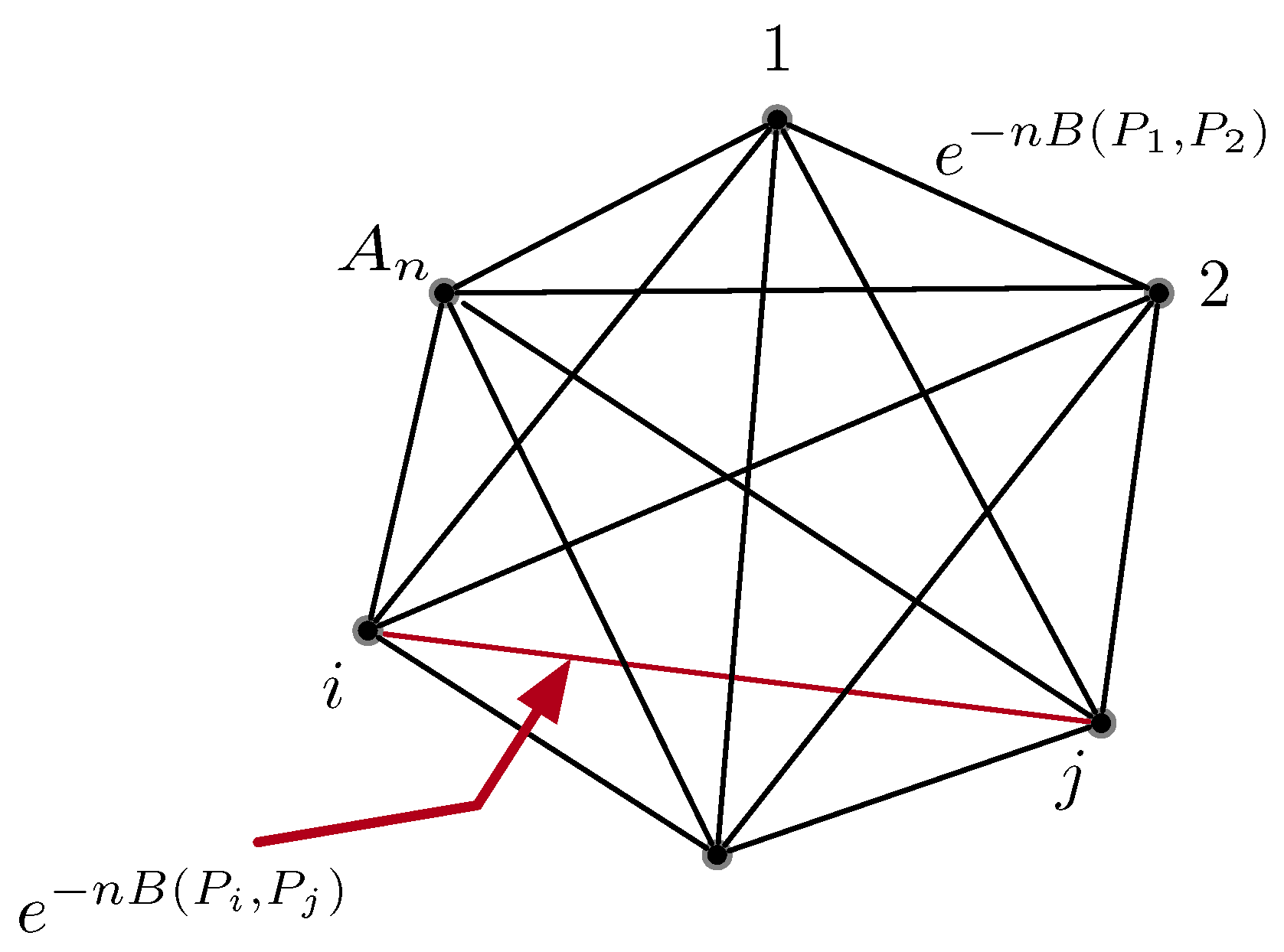
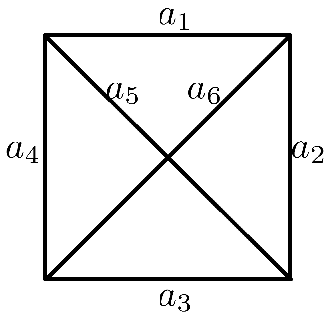
| ; A complete graph with k nodes and edge weights between node . | |
| A cycle of length r represented by the set of its vertices and edges, respectively. | |
| i-th vertex of the cycle . | |
| Set of cycles of length r in the complete graph . | |
| Number of cycles of length r in a complete graph . | |
| ; Gain of a cycle which we define as the product of the edge weights within the cycle c. | |
| AM-GM inequality | Refers to the following inequality . |
Disclaimer/Publisher’s Note: The statements, opinions and data contained in all publications are solely those of the individual author(s) and contributor(s) and not of MDPI and/or the editor(s). MDPI and/or the editor(s) disclaim responsibility for any injury to people or property resulting from any ideas, methods, instructions or products referred to in the content. |
© 2022 by the authors. Licensee MDPI, Basel, Switzerland. This article is an open access article distributed under the terms and conditions of the Creative Commons Attribution (CC BY) license (https://creativecommons.org/licenses/by/4.0/).
Share and Cite
Shahi, S.; Tuninetti, D.; Devroye, N. The Strongly Asynchronous Massive Access Channel. Entropy 2023, 25, 65. https://doi.org/10.3390/e25010065
Shahi S, Tuninetti D, Devroye N. The Strongly Asynchronous Massive Access Channel. Entropy. 2023; 25(1):65. https://doi.org/10.3390/e25010065
Chicago/Turabian StyleShahi, Sara, Daniela Tuninetti, and Natasha Devroye. 2023. "The Strongly Asynchronous Massive Access Channel" Entropy 25, no. 1: 65. https://doi.org/10.3390/e25010065
APA StyleShahi, S., Tuninetti, D., & Devroye, N. (2023). The Strongly Asynchronous Massive Access Channel. Entropy, 25(1), 65. https://doi.org/10.3390/e25010065