
Financial Fraud Detection and Prediction in Listed Companies Using SMOTE and Machine Learning Algorithms


Abstract
:1. Introduction
- We have comprehensively investigated the issues of fraud detection in listed companies related to imbalanced data classification in machine learning.
- The number of financial fraud records is 18,060 and the number of indicators is 353. This means that a large amount of data is the basis of our research; thus increasing the probability of accurate prediction.
- We used the Synthetic Minority Oversampling Technique (SMOTE) to address imbalance in the data set.
- We proposed the new framework when we chose reasonable indicators which have a big impact on the type of companies, such as Logistic Regression (LR), Random Forest (RF), Gradient Boosting Decision Tree (GBDT), Decision Tree (DT), and Extreme Gradient Boosting (XGBOOST).
- We carried out grid search that can choose the best parameter when constructing machine learning models, including Logistic Regression (LR), Support Vector Machine (SVM), Random Forest (RF), and Extreme Gradient Boosting (XGBOOST).
- We implemented voting classifier method with several ML methods to get more reasonable and scientific results compared with single classification models of reviews.
2. Related Work
3. Research Methology
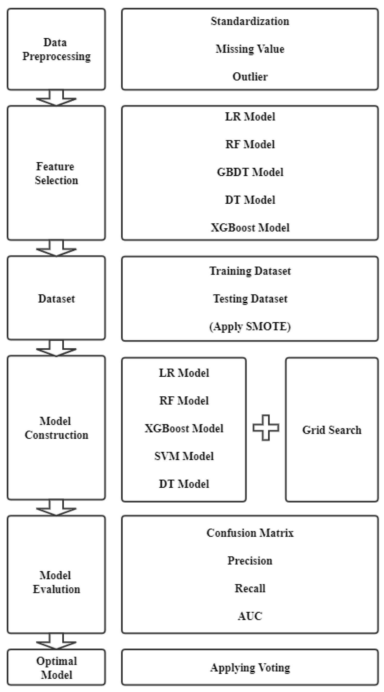
3.1. Framework
3.2. Dataset and Data Pre-Processing
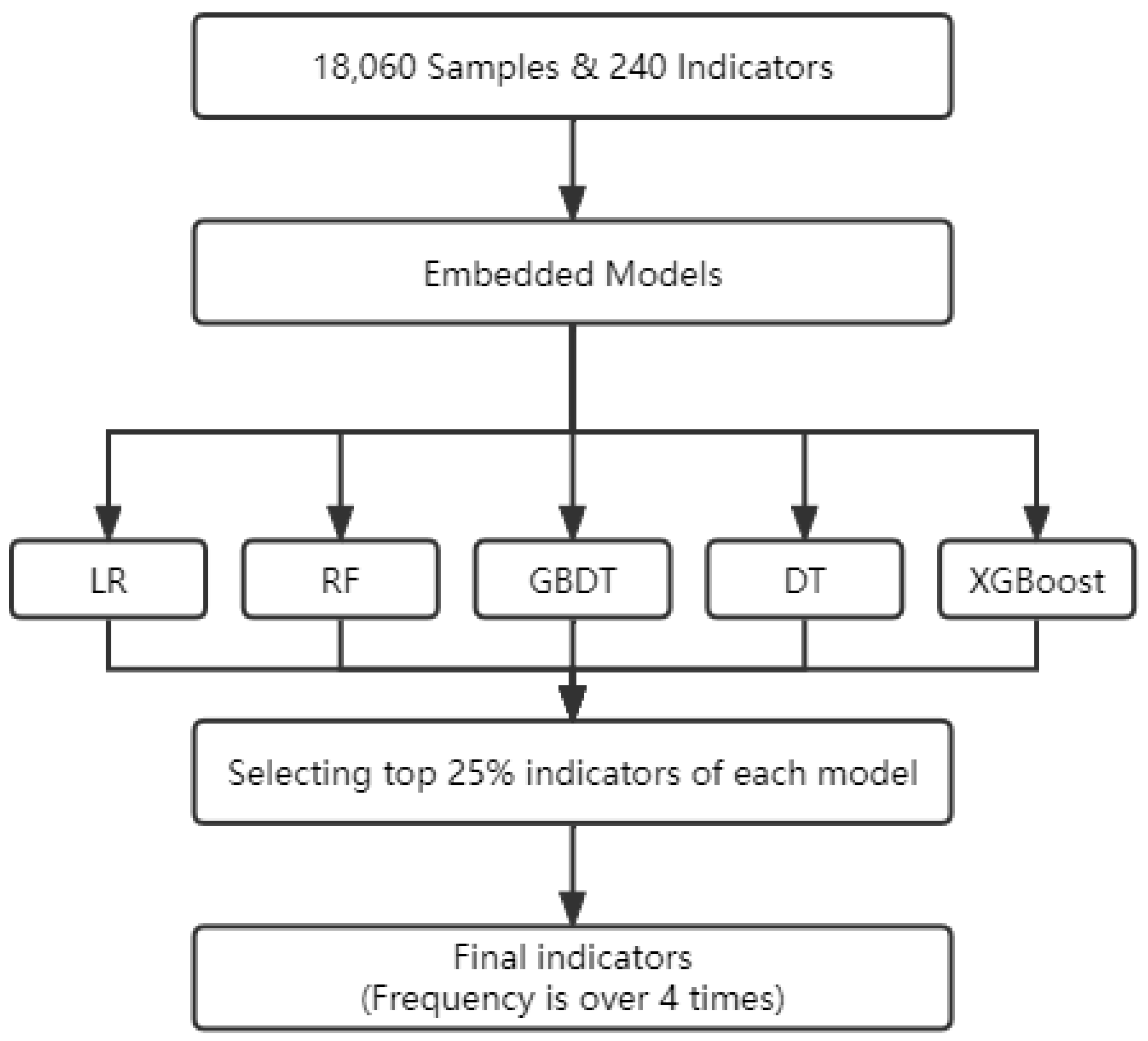
3.3. Feature Selection
3.4. Sampling Method
3.5. Machine Learning Models
3.6. Setting Parameters of Machine Learning Algorithm
3.7. Voting Classifier
3.8. Performance Metrics
- True Positive (): legitimate records that are accurately labeled as legitimate.
- True Negative (): fraudulent records that are accurately labeled as fraudulent.
- False Positive (): fraudulent records that are incorrectly labeled as legitimate.
- False Negative (): legitimate records that are incorrectly classified as fraudulent records.
4. Results and Discussions
4.1. Experiment Setup
4.2. Results and Discussions
- Deep learning is more effective in text, video, and image processing compared with classification.
- The importance of each indicator is not clear, because neural networks pay attention to the model framework. It is difficult to prevent and get information of the state of the finances.
- When we conduct deep learning, we cannot know how to predict according to parameters and which indicators are essential for management because it is not easy to explain the connections between neurons.
5. Conclusions
- In terms of collecting data, we ought to collect data as much as possible.
- In term of model application, the financial fraud identification and prediction model can be used not only in the stock market but also in company operations for oversight of the company’s financial status at anytime and anywhere.
- In term of model validation, we plan to collect financial indicators of other listed companies in various industries and apply the model to validate the model effect and ensure its reliability by repeating the experiment.
Author Contributions
Funding
Institutional Review Board Statement
Informed Consent Statement
Data Availability Statement
Conflicts of Interest
References
- Reurink, A. Financial fraud: A literature review. J. Econ. Surv. 2018, 32, 1292–1325. [Google Scholar] [CrossRef] [Green Version]
- Restya, W.P.D. Corrupt behavior in a psychological perspective. Asia Pac. Fraud. J. 2019, 4, 177–182. [Google Scholar] [CrossRef]
- Treadway, J.C.; Thompson, G.; Woolworth, F.W. Comment letters to the National Commission on Commission on Fraudulent Financial Reporting; Treadway Commission: New York, NY, USA, 1987; Volume 2. [Google Scholar]
- Li, R.H. A study for establishing a fraud audit. Audit. Econ. Res. 2002, 17, 31–35. [Google Scholar]
- Handoko, B.L.; Warganegara, D.L.; Ariyanto, S. The impact of financial distress, stability, and liquidity on the likelihood of financial statement fraud. Palarch’s J. Archaeol. Egypt/Egyptology 2020, 17, 2383–2394. [Google Scholar]
- Peng, Z. A Ripple in the Muddy Waters: The Luckin Coffee Scandal and Short Selling Attacks. Available online: https://ssrn.com/abstract=3672971 (accessed on 1 August 2020).
- Li, Y. Research on the Effectiveness of China’s A-share Main Board Market. In E3S Web of Conferences; EDP Sciences: Les Ulis, France, 2021; Volume 235. [Google Scholar]
- Zhu, X.; Ao, X.; Qin, Z.; Chang, Y.; Liu, Y.; He, Q.; Li, J. Intelligent financial fraud detection practices in post-pandemic era. Innovation 2021, 2, 100176. [Google Scholar] [CrossRef]
- Mohammed, R.A.; Wong, K.W.; Shiratuddin, M.F.; Wang, X. Scalable machine learning techniques for highly imbalanced credit card fraud detection: A comparative study. In Pacific Rim International Conference on Artificial Intelligence; Springer: Cham, Switzerland, 2018; pp. 237–246. [Google Scholar]
- Kaur, H.; Pannu, H.S.; Malhi, A.K. A systematic review on imbalanced data challenges in machine learning: Applications and solutions. Acm Comput. Surv. (CSUR) 2020, 52, 1–36. [Google Scholar] [CrossRef] [Green Version]
- Ganganwar, V. An overview of classification algorithms for imbalanced data set. Int. J. Emerg. Technol. Adv. Eng. 2012, 2, 42–47. [Google Scholar]
- Neumann, J.; Schnörr, C.; Steidl, G. Combined SVM-based feature selection and classification. Mach. Learn. 2005, 61, 129–150. [Google Scholar] [CrossRef] [Green Version]
- Tang, J.; Alelyani, S.; Liu, H. Feature selection for classification: A review. Data Classif. Algorithms Appl. 2014, 37–64. [Google Scholar]
- Guyon, I.; Elisseeff, A. An introduction to variable and feature selection. J. Mach. Learn. Res. 2003, 3, 1157–1182. [Google Scholar]
- Kohavi, R.; John, G.H. Wrappers for feature subset selection. Artif. Intell. 1997, 97, 273–324. [Google Scholar] [CrossRef] [Green Version]
- Omar, N.; Jusoh, F.; Ibrahim, R.; Othman, M.S. Review of feature selection for solving classification problems. J. Inf. Syst. Res. Innov. 2013, 3, 64–70. [Google Scholar]
- Coelho, F.; Braga, A.P.; Verleysen, M. A mutual information estimator for continuous and discrete variables applied to feature selection and classification problem. Int. J. Comput. Intell. Syst. 2016, 9, 726–733. [Google Scholar] [CrossRef] [Green Version]
- Bell, T.B.; Carcello, J.V. A Decision Aid for Assessing the Likelihood of Fraudulent Financial Reporting. Audit. J. Pract. Theory 2000, 19, 169–184. [Google Scholar] [CrossRef]
- Spathis, C.T. Detecting False Financial Statements Using Published Data: Some Evidence from Greece. Manag. Audit. J. 2002, 17, 179–191. [Google Scholar] [CrossRef] [Green Version]
- Kirkos, E.; Spathis, C.; Manolopoulos, Y. Data mining techniques for the detection of fraudulent financial statements. Expert Syst. Appl. 2007, 32, 995–1003. [Google Scholar] [CrossRef]
- Skousen, C.J.; Smith, K.R.; Wright, C.J. Detecting and Predicting Financial Statement Fraud: The Effectiveness of the Fraud Triangle and SAS No. 99. Soc. Sci. Electron. Publ. 2008, 13, 53–81. [Google Scholar] [CrossRef]
- Ravisankar, P.; Ravi, V.; Rao, G.R.; Bose, I. Detection of financial statement fraud and feature selection using data mining techniques. Decis. Support Syst. 2011, 50, 491–500. [Google Scholar] [CrossRef]
- Glancy, F.H.; Yadav, S.B. A computational model for financial reporting fraud detection. Decis. Support Syst. 2011, 50, 595–601. [Google Scholar] [CrossRef]
- Chawla, N.V.; Bowyer, K.W.; Hall, L.O.; Kegelmeyer, W.P. SMOTE: Synthetic minority over-sampling technique. J. Artif. Intell. Res. 2002, 16, 321–357. [Google Scholar] [CrossRef]
- Abdoh, S.F.; Rizka, M.A.; Maghraby, F.A. Cervical Cancer Diagnosis Using Random Forest Classifier with SMOTE and Feature Reduction Techniques. IEEE Access 2018, 6, 59475–59485. [Google Scholar] [CrossRef]
- Ileberi, E.; Sun, Y.; Wang, Z. Performance Evaluation of Machine Learning Methods for Credit Card Fraud Detection Using SMOTE and AdaBoost. IEEE Access 2021, 6, 165286–165294. [Google Scholar] [CrossRef]
- Dreiseitl, S.; Ohno-Machado, L. Logistic regression and artificial neural network classification models: A methodology review. J. Biomed. Inform. 2002, 35, 352–359. [Google Scholar] [CrossRef] [Green Version]
- Speiser, J.L.; Miller, M.E.; Tooze, J.; Ip, E. A comparison of random forest variable selection methods for classification prediction modeling. Expert Syst. Appl. 2019, 134, 93–101. [Google Scholar] [CrossRef]
- Ramraj, S.; Uzir, N.; Sunil, R.; Banerjee, S. Experimenting XGBOOST algorithm for prediction and classification of different data sets. Int. J. Control. Theory Appl. 2016, 9, 651–662. [Google Scholar]
- Bhavsar, H.; Panchal, M.H. A review on support vector machine for data classification. Int. J. Adv. Res. Comput. Eng. Technol. 2012, 11, 185–189. [Google Scholar]
- Song, Y.Y.; Ying, L.U. Decision tree methods: Applications for classification and prediction. Shanghai Arch. Psychiatry 2015, 27, 130. [Google Scholar]
- Pedregosa, F.; Varoquaux, G.; Gramfort, A.; Michel, V.; Thirion, B.; Grisel, O.; Blondel, M.; Prettenhofer, P.; Weiss, R.; Dubourg, V.; et al. Scikit-learn: Machine Learning in Python. J. Mach. Learn. Res. 2011, 12, 2825–2830. [Google Scholar]
- LogisticRegression. Available online: https://scikit-learn.org/stable/modules/classes.html (accessed on 29 March 2022).
- RandomForestClassifier. Available online: https://scikit-learn.org/stable/supervised_learning.html (accessed on 29 March 2022).
- SVC. Available online: https://scikit-learn.org/stable/supervised_learning.html (accessed on 29 March 2022).
- DecisionTreeClassifier. Available online: https://scikit-learn.org/stable/supervised_learning.html (accessed on 29 March 2022).
- Kabari, L.G.; Onwuka, U.C. Comparison of bagging and voting ensemble machine learning algorithm as a classifier. Int. J. Adv. Res. Comput. Sci. Softw. Eng. 2019, 9, 19–23. [Google Scholar]
- Randhawa, K.; Loo, C.K.; Seera, M.; Lim, C.P.; Nandi, A.K. Credit card fraud detection using AdaBoost and majority voting. IEEE Access 2018, 6, 14277–14284. [Google Scholar] [CrossRef]
- Taha, A.A.; Malebary, S.J. An intelligent approach to credit card fraud detection using an optimized light gradient boosting machine. IEEE Access 2020, 8, 25579–25587. [Google Scholar] [CrossRef]
- Khamis, H. Measures of association: How to choose? J. Diagn. Med. Sonogr. 2008, 24, 155–162. [Google Scholar] [CrossRef] [Green Version]
- Mehbodniya, A.; Alam, I.; Pande, S.; Neware, R.; Rane, K.P.; Shabaz, M.; Madhavan, M.V. Financial fraud detection in healthcare using machine learning and deep learning techniques. Secur. Commun. Netw. 2021, 2021, 9293877. [Google Scholar] [CrossRef]
- Gupta, R.Y.; Mudigonda, S.S.; Baruah, P.K. A comparative study of using various machine learning and deep learning-based fraud detection models for universal health coverage schemes. Int. J. Eng. Trends Technol. 2021, 69, 96–102. [Google Scholar] [CrossRef]
- Mathew, A.; Amudha, P.; Sivakumari, S. Deep learning techniques: An overvie. In International Conference on Advanced Machine Learning Technologies and Applications; Springer: Singapore, 2020; pp. 599–608. [Google Scholar]


| Algorithm | Parameter | Value |
|---|---|---|
| LR | Penalty | [‘l1’,‘l2’] |
| C | [0.01,0.05,0.1,0.5,10,50,100] | |
| Solver | [‘liblinear’,‘lbfgs’] | |
| RF | Criterion | [‘gini’,‘entropy’] |
| Max_features | range(1,len(features)) | |
| N_estimators | [1,10,20,50,100] | |
| XGBOOST | Max_depth | range(1,len(features)) |
| Learning_rate | [0.01,0.1,0.5,1] | |
| Gamma | [0.01,0.05,0.1,0.5,10,50,100] | |
| SVM | C | [0.01,0.05,0.1,0.5,10,50,100] |
| Gamma | [0.01,0.05,0.1,0.5,10,50,100] | |
| DT | Criterion | [‘gini’,‘entropy’] |
| Max_features | range(1,len(features)) |
| Indicator | Meaning | Unit |
|---|---|---|
| RETAINED_EARNINGS | Undistributed profits | CNY |
| PUR_FIX_ASSETS_OTH | Cash paid for fixed assets, intangible assets and other long-term assets | CNY |
| CIP | Construction work in process | CNY |
| ADVANCE_RECEIPTS | Deposit received | CNY |
| NOPERATE_EXP | Non-business expenditure | CNY |
| C_PAID_TO_FOR_EMPL | Cash received relating to operating activities | CNY |
| INVENTORIES | Inventory | CNY |
| MINORITY_INT | Minority equity | CNY |
| BIZ_TAX_SURCHG | Business taxes and surcharges | CNY |
| ASSETS_DISP_GAIN | Gain on disposal of assets | CNY |
| BASIC_EPS | Primary earnings per share | CNY |
| COMPR_INC_ATTR_M_S | Total comprehensive income attributable to minority shareholders | CNY |
| N_CF_OPA_R | Operating cash flow (operating income) | CNY |
| Pointbiserial Correlation Coefficient | |||||||
|---|---|---|---|---|---|---|---|
| y | 0.908 | 0.839 | 0.491 | 0.665 | 0.829 | 0.989 | 0.552 |
| y | 0.757 | 0.432 | 0.769 | 0.605 | 0.116 | 0.737 |
| Original | The number of legitimate records | The number of fraudulent records |
|---|---|---|
| Training data set | 12,526 | 116 |
| Testing data set | 5354 | 64 |
| After | The number of legitimate records | The number of fraudulent records |
| Training data set | 12,526 | 12,526 |
| Testing data set | 5354 | 5354 |
| Algorithm | The Value of AUC (Imbalanced Data Set) | The Value of AUC (Balanced Data Set) |
|---|---|---|
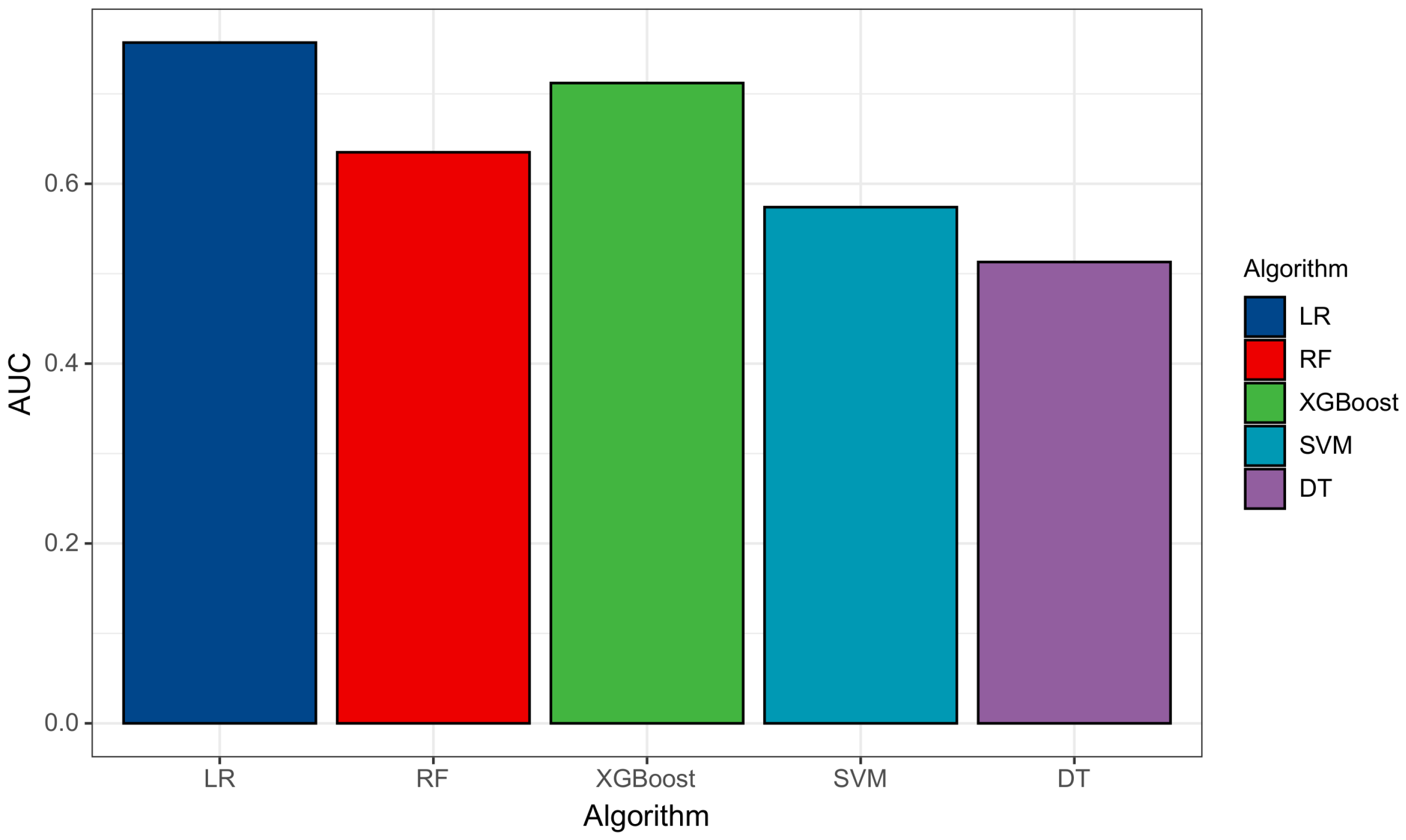
| LR | 0.719 | 0.757 |
| RF | 0.562 | 0.635 |
| XGBOOST | 0.690 | 0.712 |
| SVM | 0.509 | 0.574 |
| DT | 0.505 | 0.513 |
| Algorithm | Parameter | Value |
|---|---|---|
| LR | Penalty | l2 |
| C | 50 | |
| Solver | lbfgs | |
| RF | Criterion | gini |
| Max_features | 1 | |
| N_estimators | 50 | |
| XGBOOST | Max_depth | 7 |
| Learning_rate | 0.5 | |
| Gamma | 0.05 | |
| SVM | C | 100 |
| Gamma | 100 | |
| DT | Criterion | gini |
| Max_features | 9 |
| Algorithm | ||||
|---|---|---|---|---|
| LR | 3590 | 1773 | 15 | 40 |
| RF | 5362 | 1 | 55 | 0 |
| XGBOOST | 5358 | 5 | 55 | 0 |
| SVM | 5289 | 74 | 55 | 0 |
| DT | 5323 | 40 | 54 | 1 |
| Algorithm | AUC | Training Time | Testing Time | |||
|---|---|---|---|---|---|---|
| LR | 66.999% | 99.584% | 66.940% | 0.757 | 0.05 s | 0.01 s |
| RF | 98.966% | 98.985% | 99.981% | 0.635 | 0.26 s | 0.01 s |
| XGBOOST | 98.893% | 98.984% | 99.907% | 0.712 | 1.46 s | 0.02 s |
| SVM | 97.619% | 98.971% | 98.620% | 0.574 | 2.49 s | 0.01 s |
| DT | 98.265% | 98.996% | 99.254% | 0.513 | 0.03 s | 0.01 s |
| Algorithm | AUC | Training Time | Testing Time | |||
|---|---|---|---|---|---|---|
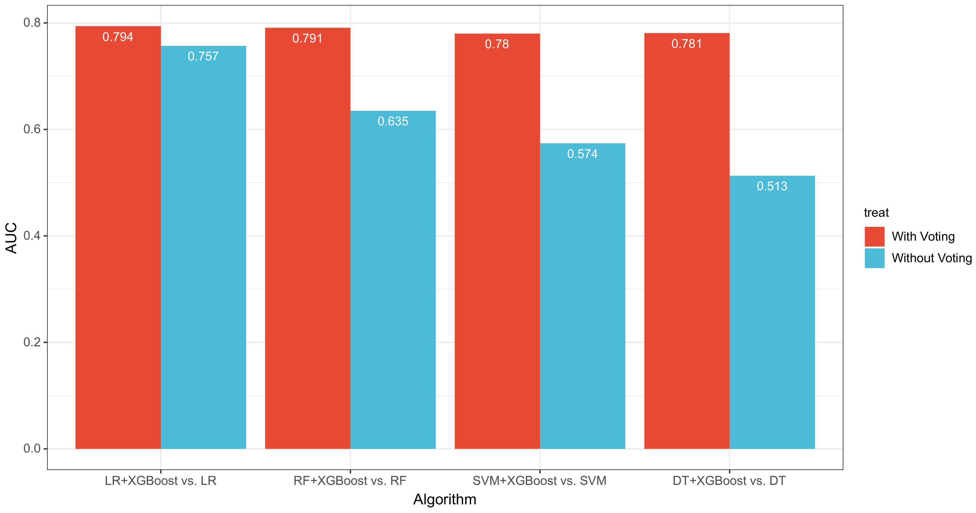
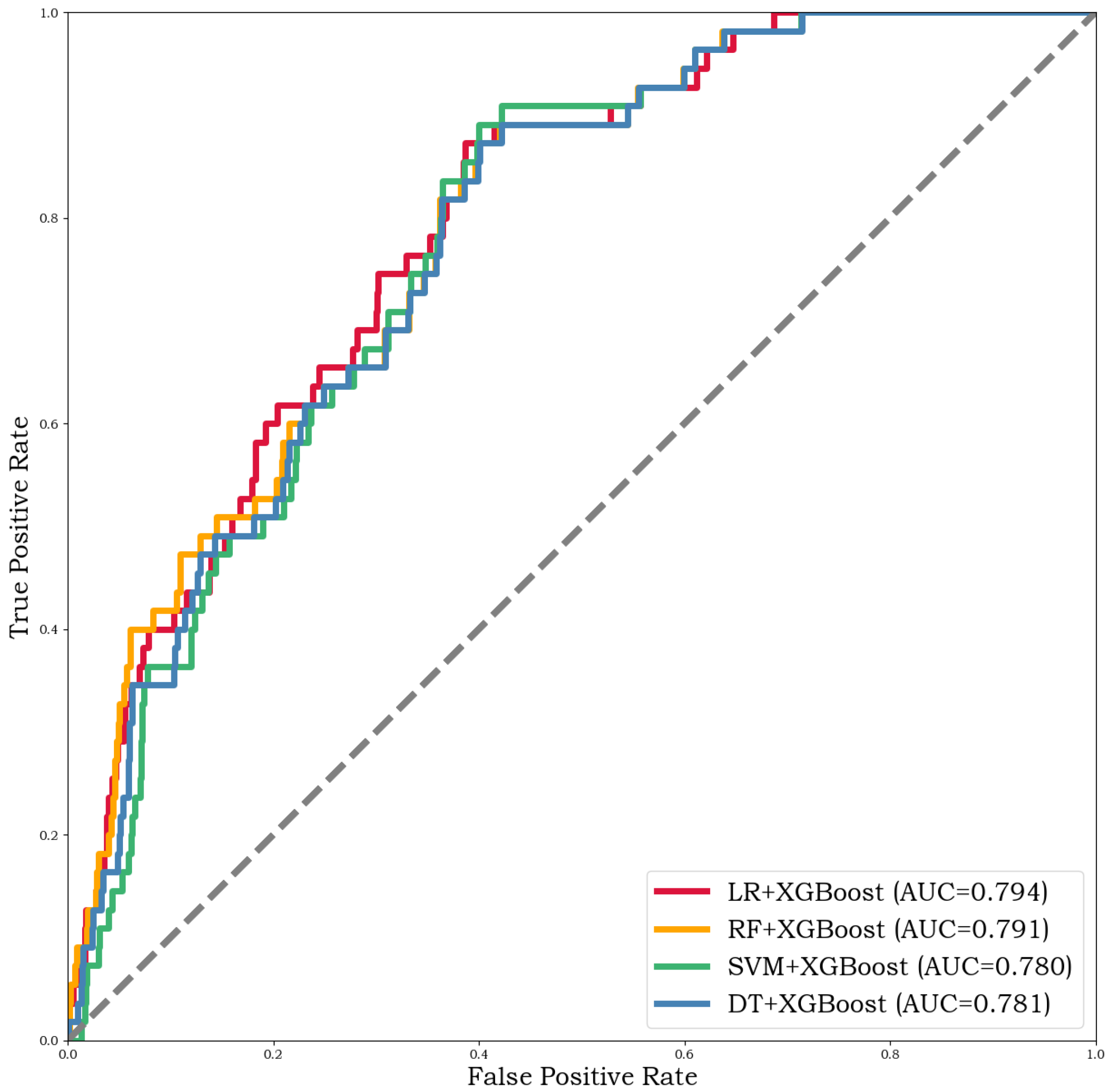
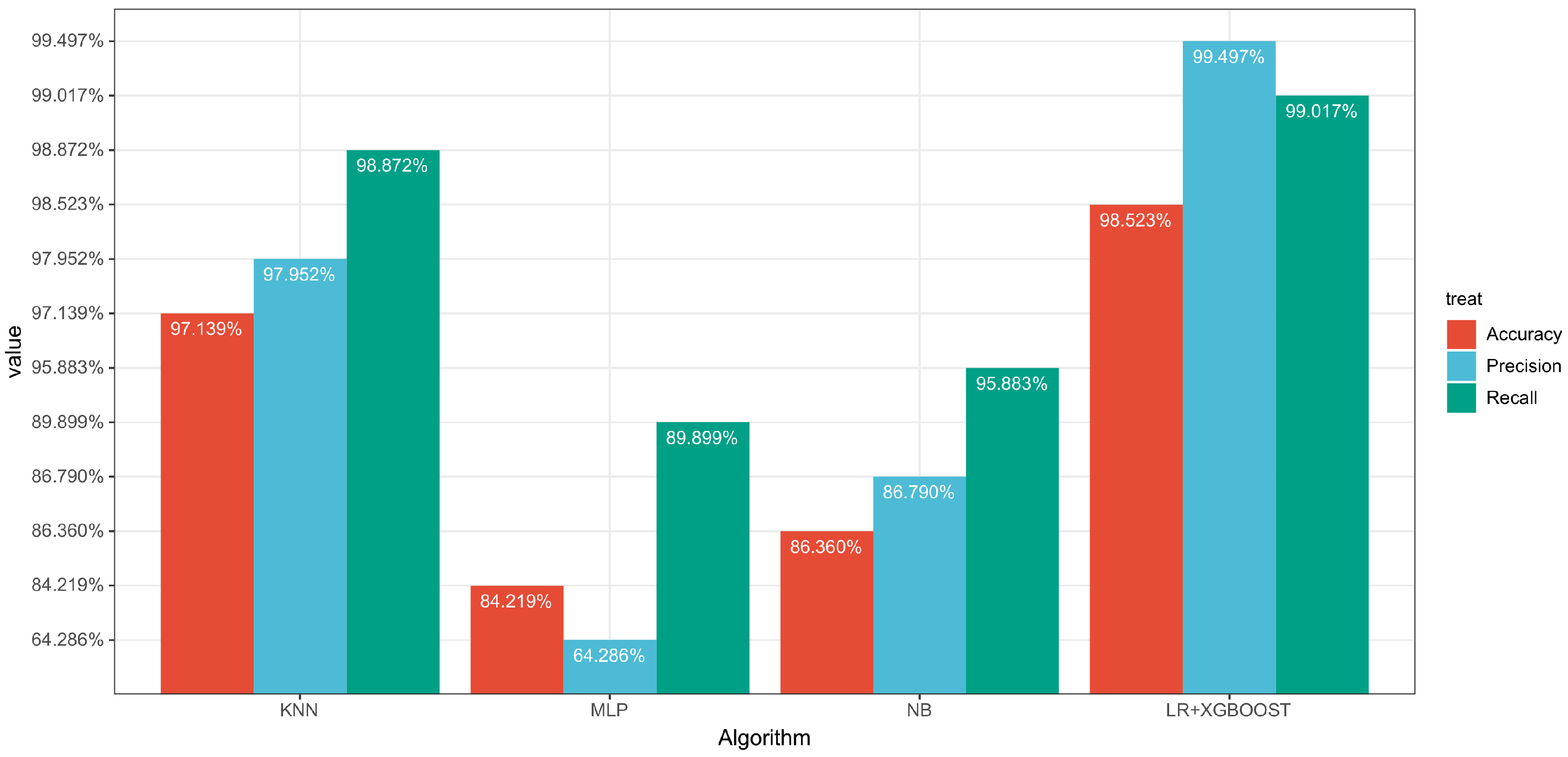
| LR + XGBOOST | 98.523% | 99.017% | 99.497% | 0.794 | 1.54 s | 0.01 s |
| RF + XGBOOST | 98.616% | 99.036% | 99.571% | 0.791 | 1.75 s | 0.05 s |
| SVM + XGBOOST | 97.933% | 98.974% | 98.937% | 0.780 | 12.34 s | 0.71 s |
| DT + XGBOOST | 98.154% | 98.995% | 99.142% | 0.781 | 1.54 s | 0.01 s |
Publisher’s Note: MDPI stays neutral with regard to jurisdictional claims in published maps and institutional affiliations. |
© 2022 by the authors. Licensee MDPI, Basel, Switzerland. This article is an open access article distributed under the terms and conditions of the Creative Commons Attribution (CC BY) license (https://creativecommons.org/licenses/by/4.0/).
Share and Cite
Zhao, Z.; Bai, T. Financial Fraud Detection and Prediction in Listed Companies Using SMOTE and Machine Learning Algorithms. Entropy 2022, 24, 1157. https://doi.org/10.3390/e24081157
Zhao Z, Bai T. Financial Fraud Detection and Prediction in Listed Companies Using SMOTE and Machine Learning Algorithms. Entropy. 2022; 24(8):1157. https://doi.org/10.3390/e24081157
Chicago/Turabian StyleZhao, Zhihong, and Tongyuan Bai. 2022. "Financial Fraud Detection and Prediction in Listed Companies Using SMOTE and Machine Learning Algorithms" Entropy 24, no. 8: 1157. https://doi.org/10.3390/e24081157
APA StyleZhao, Z., & Bai, T. (2022). Financial Fraud Detection and Prediction in Listed Companies Using SMOTE and Machine Learning Algorithms. Entropy, 24(8), 1157. https://doi.org/10.3390/e24081157