Figure 1.
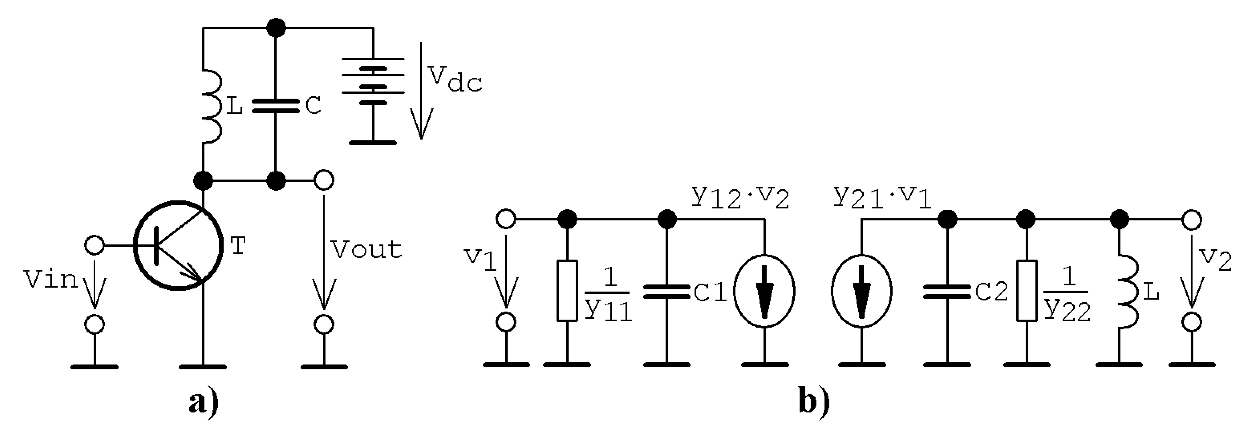
General circuit concepts analyzed in this paper: (a) fundamental cell of class C amplifier, (b) equivalent schematic of class C amplifier for useful small-amplitude AC (Alternating Current) signals.
Figure 1.
General circuit concepts analyzed in this paper: (a) fundamental cell of class C amplifier, (b) equivalent schematic of class C amplifier for useful small-amplitude AC (Alternating Current) signals.
Figure 2.
Plane projection v1 vs. v2 (black) and rainbow colored three-dimensional perspective views on the typical strange attractors generated by: (a) parameter set Ψ1 substituted into the expression (1), (b) parameter set Ψ1 substituted into system (6), (c) parameter set Ψ2 substituted into differential Equation (1), (d) parameter set Ψ2 substituted into jerk dynamics (6), (e) parameter set Ψ3 numerically integrated using Equation (1), (f) integration of system (1) with parameter set Ψ4, (g) parameter set Ψ5 substituted into Equation (1), and (h) parameter set Ψ6 substituted into system (1) and integrated.
Figure 3.
Sensitivity to tiny changes of initial condition demonstrated for first case of chaotic system: starting situation (red points), short time evolution (green points), average time evolution (blue dots) and long time separation (black dots). Nominal starting position is chosen as follows: (a) x0 = (1, 0, 0)T, (b) x0 = (−1, 0, 0)T, (c) x0 = (0, −1, 0)T and (d) x0 = (0, 1, 0)T. Magnified areas showing states are demonstrated.
Figure 4.
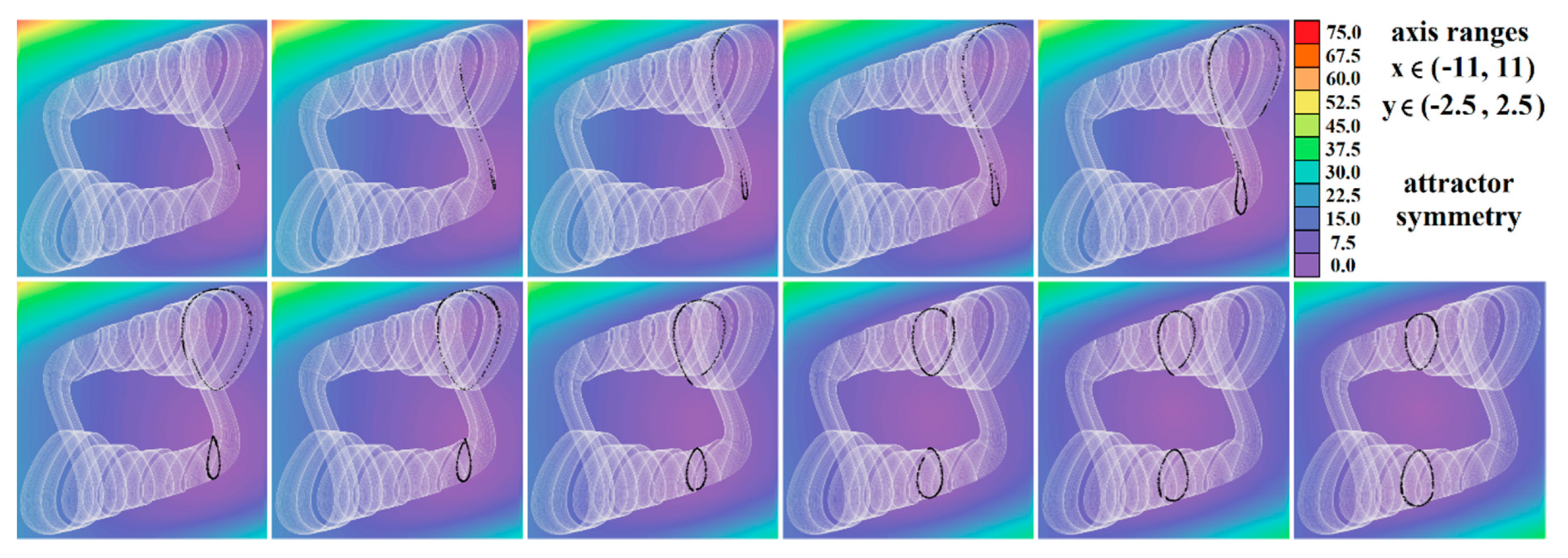
Horizontal state space slices given by z = const. showing kinetic energy distribution of typical chaotic attractors of case Ψ1 system, associated Poincaré sections (black dots). Figures sorted from left to right and up to down: z = −0.9, z = −0.7, z = −0.5, z = −0.2, z = 0, z = 0.3, z = 1, z = 1.5, z = 2, z = 2.4, and z = 2.47.
Figure 4.
Horizontal state space slices given by z = const. showing kinetic energy distribution of typical chaotic attractors of case Ψ1 system, associated Poincaré sections (black dots). Figures sorted from left to right and up to down: z = −0.9, z = −0.7, z = −0.5, z = −0.2, z = 0, z = 0.3, z = 1, z = 1.5, z = 2, z = 2.4, and z = 2.47.
Figure 5.
Horizontal state space slices defined by the plane z = const. and providing dynamical energy distribution of typical chaotic attractors of case Ψ2 system (white curve), associated Poincaré sections (black dots). Figures sorted from left to right and up to down: z = −3.3, z = −3, z = −2.5, z = −2, z = −1.5, z = −1, z = −0.8, z = −0.6, z = −0.4, z = −0.2, and z = 0.
Figure 6.
Horizontal state space slices given by plane z = const. providing rainbow scaled dynamical energy distribution of the typical chaotic attractors of case Ψ3 system, associated Poincaré sections (black dots). Individual figures are sorted from left to right and up to down with respect to the planes: z = −9.4, z = −9, z = −8.5, z = −8, z = −7, z = −6.5, z = −6, z = −4, z = −2, z = −1, and z = 0.
Figure 7.
Horizontal state space slices given by plane z = const. providing rainbow scaled dynamical energy distribution of the typical chaotic attractors of case Ψ4 system (white trajectory), and associated Poincaré sections (black dots). Figures sorted from left to right and up to down: z = −0.4, z = −0.2, z = 0, z = 0.2, z = 0.3, z = 0.5, z = 0.8, z = 1.2, z = 1.6, z = 2, and z = 2.5.
Figure 8.
Horizontal state space slices given by plane z = const. providing rainbow scaled dynamical energy distribution of the typical chaotic attractors of case Ψ5 system (white trajectory), and associated Poincaré sections (black dots). Individual figures are sorted from left to right and up to down: z = −1, z = −0.8, z = −0.6, z = −0.2, z = 0.4, z = 0.6, z = 1, z = 1.5, z = 2, z = 2.5, and z = 2.9.
Figure 9.
Horizontal state space slices defined by plane z = const. providing rainbow scaled dynamical energy distribution of typical chaotic attractors of case Ψ6 system (white state trajectory), associated Poincaré sections (black dots). Figures sorted from left to right and up to down are given by: z =−3.3, z = −2.7, z = −2, z = −1.2, z = −0.7, z = 0, z = 0.4, z = 1, z = 1.7, z = 2.3, and z = 3.3.
Figure 10.
Horizontal state space slices given by plane z = const. providing rainbow scaled dynamical energy distribution of the typical chaotic attractors of case Ψ7 system (white trajectory), and associated Poincaré sections (black dots). Individual figures sorted from left to right and up to down are given by: z = −1.4, z = −1, z = −0.5, z = −0.2, z = 0, z = 0.2, z = 0.5, z = 1, z = 1.5, z = 1.8, z = 2.2, and z = 2.7.
Figure 11.
Rainbow scaled surface-contour plot of the largest Lyapunov exponent as two-dimensional function of nonlinear feedback, calculated for Ψ1 case of chaotic circuit and total range of parameters is a∈(0, 3) and b∈(−3, 0).
Figure 11.
Rainbow scaled surface-contour plot of the largest Lyapunov exponent as two-dimensional function of nonlinear feedback, calculated for Ψ1 case of chaotic circuit and total range of parameters is a∈(0, 3) and b∈(−3, 0).
Figure 12.
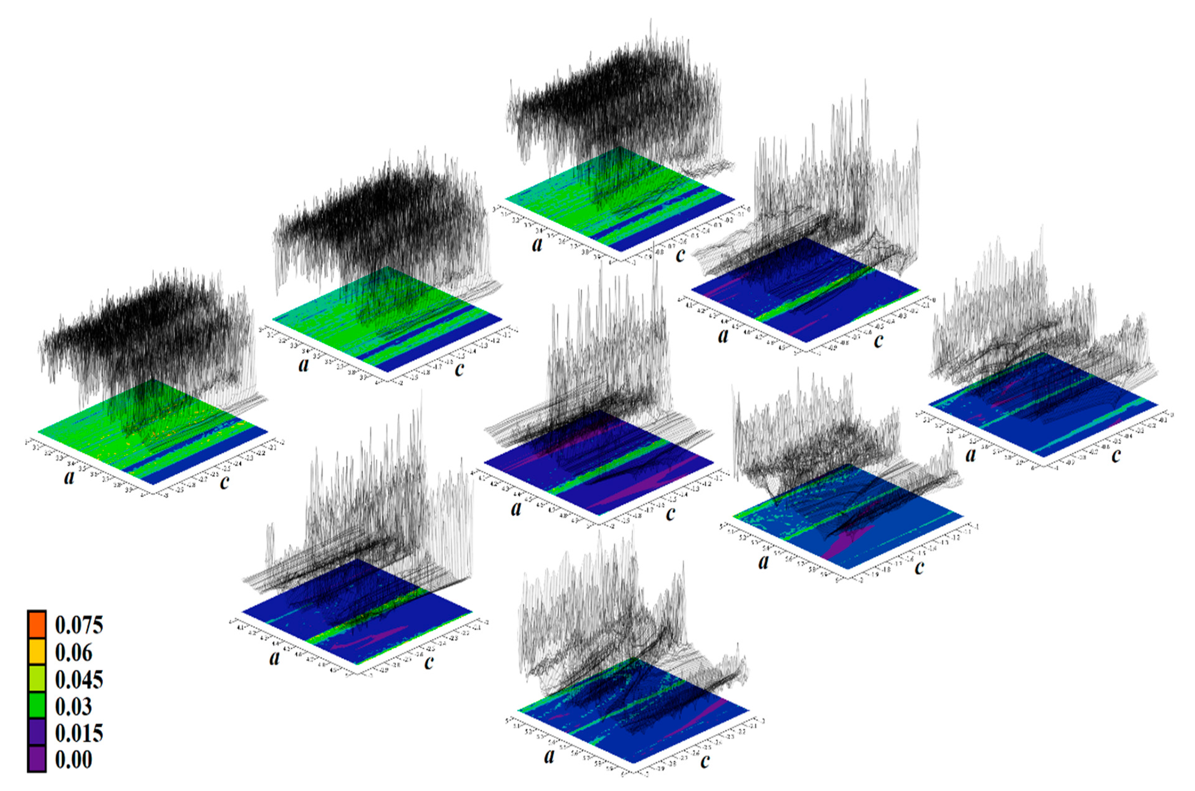
Rainbow scaled surface-contour plot of the largest Lyapunov exponent as two-dimensional function of nonlinear feedback, area covering both Ψ2, Ψ5, and Ψ7 with dissipation coefficient y11 = 0.4, total range of parameters is c∈(2, 5) and e∈(−3, 0).
Figure 12.
Rainbow scaled surface-contour plot of the largest Lyapunov exponent as two-dimensional function of nonlinear feedback, area covering both Ψ2, Ψ5, and Ψ7 with dissipation coefficient y11 = 0.4, total range of parameters is c∈(2, 5) and e∈(−3, 0).
Figure 13.
Rainbow scaled surface-contour plot of the largest Lyapunov exponent as two-dimensional function of nonlinear feedback, area covering case Ψ3 and total range of parameters is a∈(3, 6) along with b∈(−3, 0).
Figure 13.
Rainbow scaled surface-contour plot of the largest Lyapunov exponent as two-dimensional function of nonlinear feedback, area covering case Ψ3 and total range of parameters is a∈(3, 6) along with b∈(−3, 0).
Figure 14.
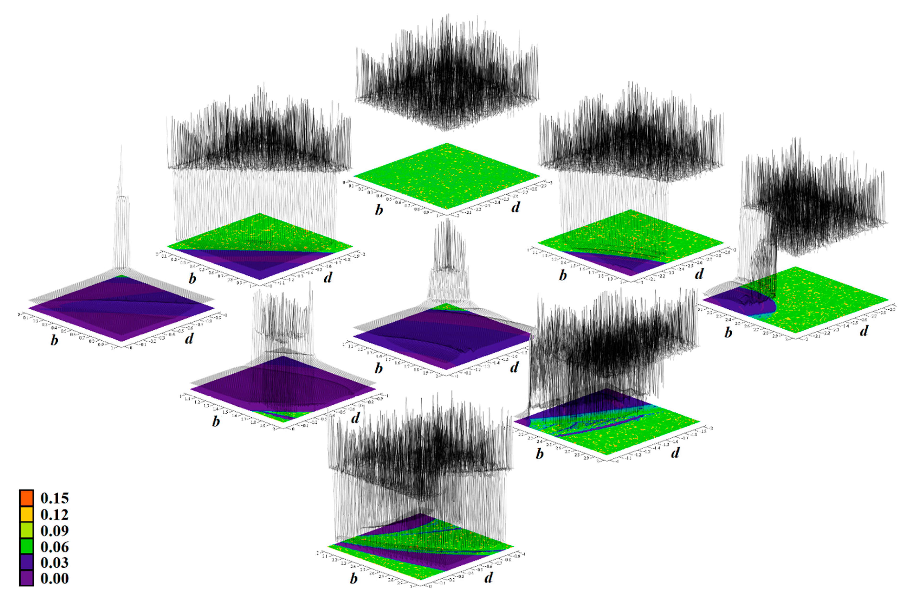
Rainbow scaled surface-contour plot of the largest Lyapunov exponent as two-dimensional function of nonlinear feedback, area covering case Ψ4 and total range of parameters is b∈(0, 3) along with d∈(−3, 0).
Figure 14.
Rainbow scaled surface-contour plot of the largest Lyapunov exponent as two-dimensional function of nonlinear feedback, area covering case Ψ4 and total range of parameters is b∈(0, 3) along with d∈(−3, 0).
Figure 15.
Rainbow scaled surface-contour plot of the largest Lyapunov exponent as two-dimensional function of nonlinear feedback, area covering case Ψ6 and total range of parameters is a∈(1, 4) along with e∈(−3, 0).
Figure 15.
Rainbow scaled surface-contour plot of the largest Lyapunov exponent as two-dimensional function of nonlinear feedback, area covering case Ψ6 and total range of parameters is a∈(1, 4) along with e∈(−3, 0).
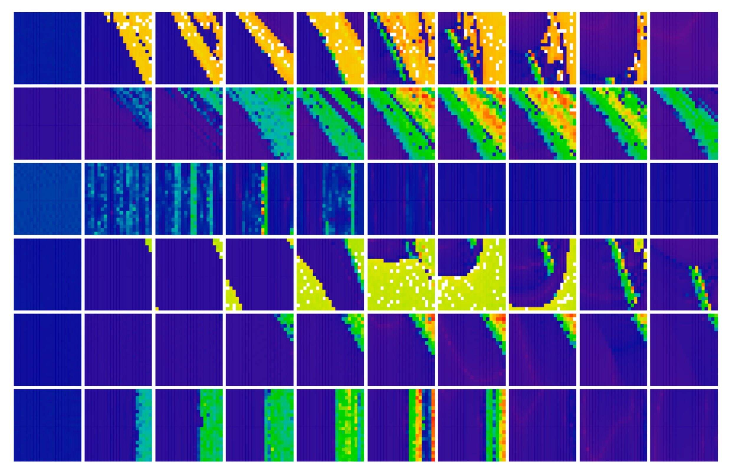
Figure 16.
Rainbow scaled plot showing flow quantification for the individual cases Ψ1–6 (rows 1 to 6) of chaotic class C amplifier and increased value of system dissipation y11 = 0, 0.1, 0.2, 0.3, 0.4, 0.5, 0.6, 0.7, 0.8, 0.9 (columns from left to right), see text for better clarification.
Figure 16.
Rainbow scaled plot showing flow quantification for the individual cases Ψ1–6 (rows 1 to 6) of chaotic class C amplifier and increased value of system dissipation y11 = 0, 0.1, 0.2, 0.3, 0.4, 0.5, 0.6, 0.7, 0.8, 0.9 (columns from left to right), see text for better clarification.
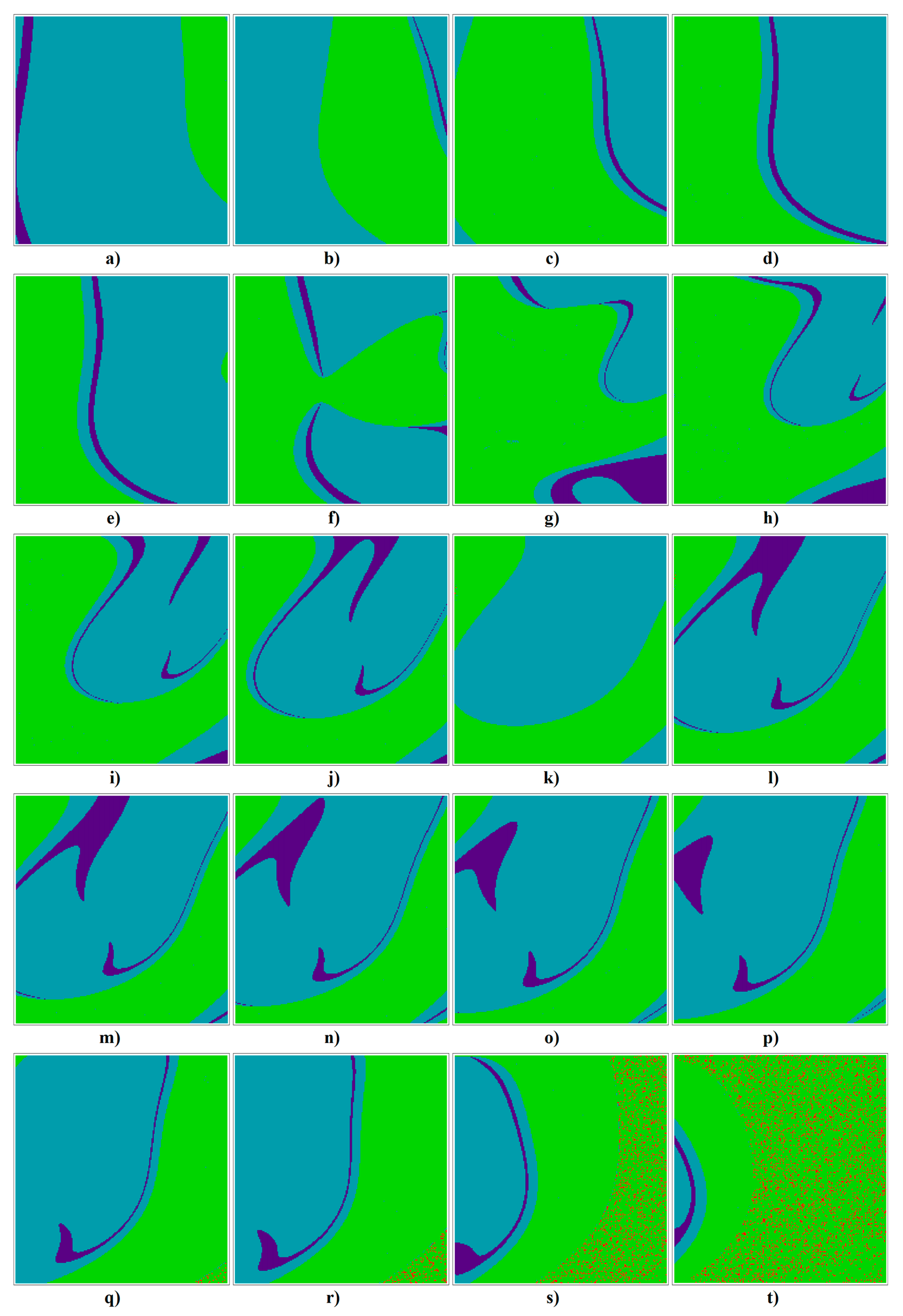
Figure 17.
Colored basins of attraction, individual slices are the horizontal planes: (a) z0 = −3, (b) z0 = −2.5, (c) z0 = −2, (d) z0 = −1.5, (e) z0 = −1.25, (f) z0 = −1, (g) z0 = −0.75, (h) z0 = −0.5, (i) z0 = −0.3, (j) z0 = −0.1, (k) z0 = 0.0, (l) z0 = 0.1, (m) z0 = 0.2, (n) z0 = 0.3, (o) z0 = 0.4, (p) z0 = 0.5, (q) z0 = 0.75, (r) z0 = 1.0, (s) z0 = 1.5, and (t) z0 = 2.
Figure 18.
Idealized circuit realization of a chaotic system with the emulated bipolar transistor stage: (
a) case
Ψ1 system with parameters taken from
Table 1, (
b) case
Ψ3 system with parameter set taken from
Table 1, (
c) Monge projections
vy1 vs.
vx1 (blue) and
iL1 vs.
vx1 (red), (
d) frequency spectrum of generated signal
vx1 (blue) and
vy1 (red). Red areas represent polynomial feedback transfer functions.
Figure 19.
Chaotic system with emulated bipolar transistor stage: (
a) circuit realization of differential Equations (1) and (3) and parameter set
Ψ3 taken from
Table 1, (
b) circuit implementation of Equations (1) and (3) and parameter set
Ψ1 or
Ψ4 taken from
Table 1.
Figure 19.
Chaotic system with emulated bipolar transistor stage: (
a) circuit realization of differential Equations (1) and (3) and parameter set
Ψ3 taken from
Table 1, (
b) circuit implementation of Equations (1) and (3) and parameter set
Ψ1 or
Ψ4 taken from
Table 1.
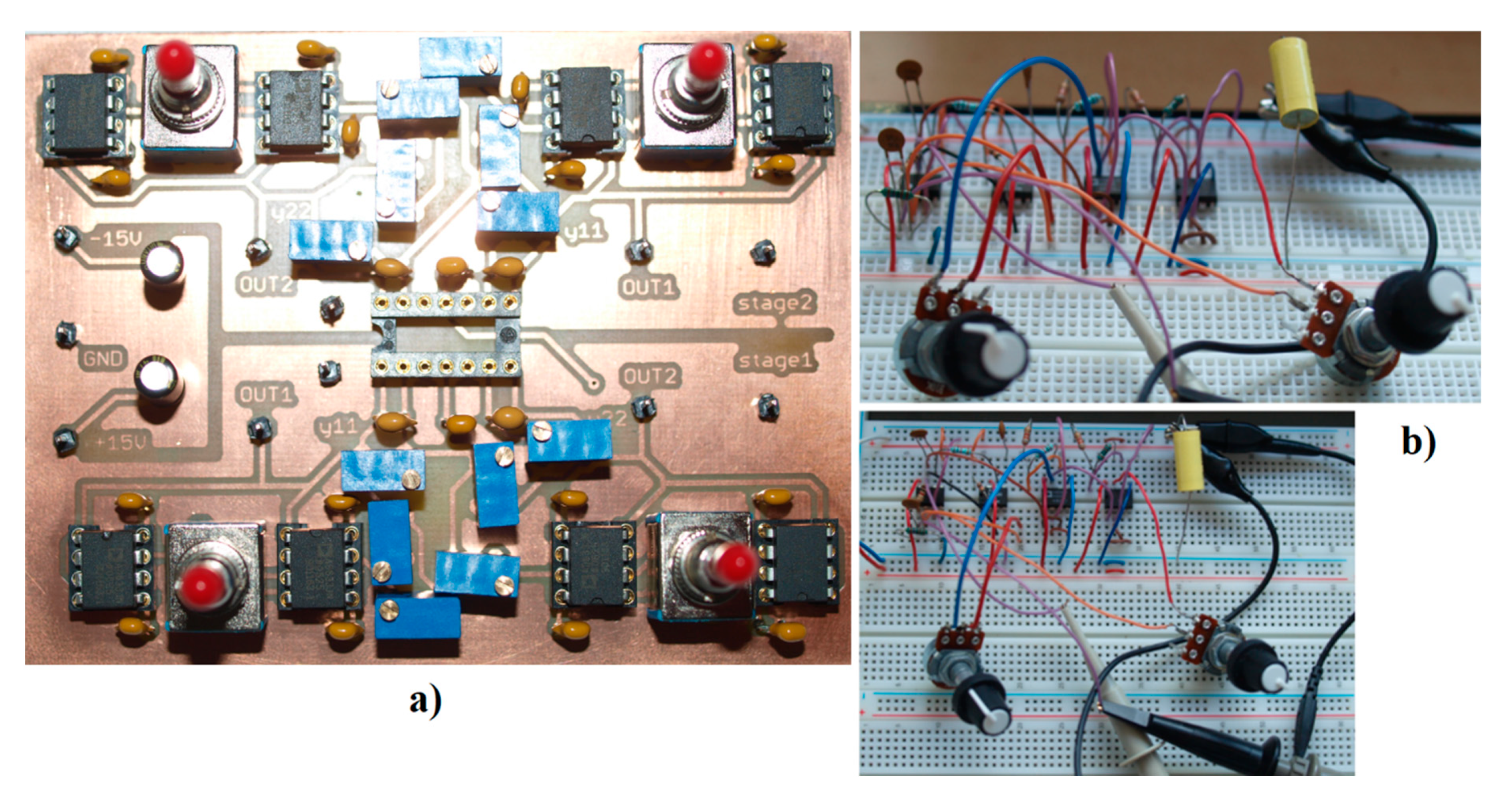
Figure 20.
Photos captured during experimental investigation: (a) PCB showing two two-ports where transconductances y12 and y21 are polynomials up to the fourth-order, (b) two views onto breadboard with designed chaotic oscillator based on generalized class C amplifier.
Figure 20.
Photos captured during experimental investigation: (a) PCB showing two two-ports where transconductances y12 and y21 are polynomials up to the fourth-order, (b) two views onto breadboard with designed chaotic oscillator based on generalized class C amplifier.
Figure 21.
Dynamical system (1) with (3) and values
Ψ3 from
Table 1, Comparison between numerical integration process (blue) and laboratory experiment (green): (
a,
b)
v1 vs.
v3 plane, (
c,
d)
v2 vs.
v3 plane, (
e,
f)
v1 vs.
v2 plane.
Figure 21.
Dynamical system (1) with (3) and values
Ψ3 from
Table 1, Comparison between numerical integration process (blue) and laboratory experiment (green): (
a,
b)
v1 vs.
v3 plane, (
c,
d)
v2 vs.
v3 plane, (
e,
f)
v1 vs.
v2 plane.
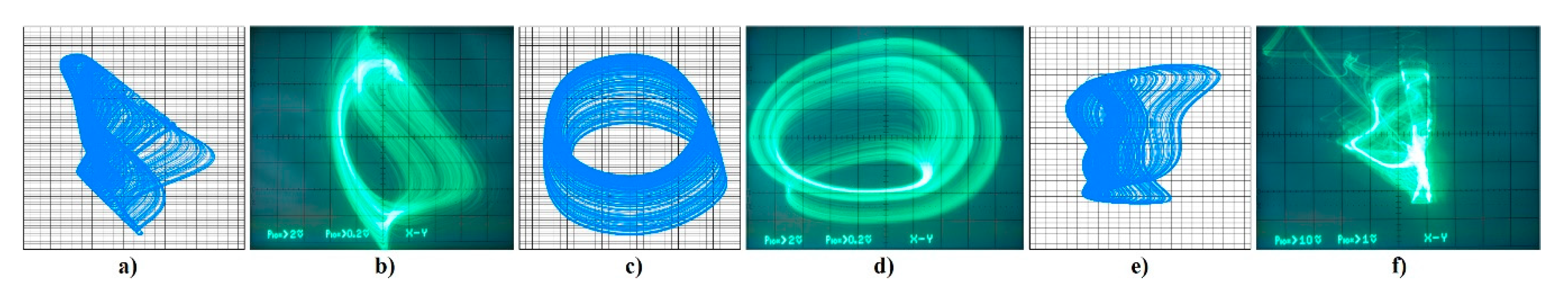
Figure 22.
Dynamical system (1) with (3) and values
Ψ1 from
Table 1, comparison between numerical integration process (blue) and laboratory experiment (green): (
a,
b)
v1 vs.
v3 plane, (
c,
d)
v1 vs.
v2 plane, (
e,
f)
v2 vs.
v3 plane.
Figure 22.
Dynamical system (1) with (3) and values
Ψ1 from
Table 1, comparison between numerical integration process (blue) and laboratory experiment (green): (
a,
b)
v1 vs.
v3 plane, (
c,
d)
v1 vs.
v2 plane, (
e,
f)
v2 vs.
v3 plane.
Figure 23.
Different Monge projections of strange attractors not mutually connected with numerical analysis of generalized chaotic class C amplifier.
Figure 23.
Different Monge projections of strange attractors not mutually connected with numerical analysis of generalized chaotic class C amplifier.
Figure 24.
Two alternative lumped circuitry implementations of class C potentially chaotic amplifier: (a) principal schematic of dynamical system with passive approximated fractional-order inductor, (b) realization based directly on the state model (20).
Figure 24.
Two alternative lumped circuitry implementations of class C potentially chaotic amplifier: (a) principal schematic of dynamical system with passive approximated fractional-order inductor, (b) realization based directly on the state model (20).
Table 1.
Numerical values of internal parameters of system (3) with mathematical orders α = β = γ = 1 that result in robust chaotic motion.
Table 1.
Numerical values of internal parameters of system (3) with mathematical orders α = β = γ = 1 that result in robust chaotic motion.
| Case | y11 | a | b | c | d | e |
|---|
| Ψ1 | 0.56 | 0 | 2.1 | 0 | −1.1 | 0 |
| Ψ2 | 0.50 | 0 | 0 | 3 | 0 | −1.5 |
| Ψ3 | 0.30 | 5 | 0 | −2 | 0 | 0 |
| Ψ4 | 0.40 | 0 | 2.7 | 0 | −2 | 0 |
| Ψ5 | 0.30 | 0 | 0 | 3 | 0 | −2 |
| Ψ6 | 0.50 | 2 | 0 | 0 | 0 | −0.5 |
| Ψ7 | 0.40 | 0 | 0 | 2 | 0 | –1 |
Table 2.
Numerical values of internal parameters of system (10) with mathematical orders α = β = γ = 1 and either (11) or (12) that result in structurally stable chaotic motion (NA means Not Available).
Table 2.
Numerical values of internal parameters of system (10) with mathematical orders α = β = γ = 1 and either (11) or (12) that result in structurally stable chaotic motion (NA means Not Available).
| Case | y11 | ϕ | ϕ1 | ϕ2 | ρ0 | ρ1 | ρ2 |
|---|
| Ψ8 | 0.56 | 1.1 | NA | NA | 1 | −4.3 | NA |
| Ψ9 | 0.5 | NA | 0.3 | 1.1 | 0.3 | 2 | −7 |
| Ψ10 | 0.3 | NA | 0.6 | 1.18 | 4.6 | 0.6 | −9.9 |
| Ψ11 | 0.3 | NA | 0.4 | 1 | 0.2 | 1.5 | −9.5 |
Table 3.
Geometric and time-domain features of generated typical strange attractors.
Table 3.
Geometric and time-domain features of generated typical strange attractors.
| Case | LLE | KYD | CD | ApEn |
|---|
| Ψ1 | 0.071 | 2.113 | 2.15 | 0.539 |
| Ψ2 | 0.156 | 2.239 | 2.24 | 0.558 |
| Ψ3 | 0.045 | 2.132 | 2.14 | 0.440 |
| Ψ4 | 0.020 | 2.050 | 2.10 | 0.503 |
| Ψ5 | 0.069 | 2.186 | 2.20 | 0.564 |
| Ψ6 | 0.047 | 2.081 | 2.15 | 0.518 |
| Ψ7 | 0.050 | 2.160 | 2.13 | 0.620 |
Table 4.
Numerical values of fully passive series-parallel circuit realization of fractional-order (FO) inductor with mathematical order 9/10, i.e., phase shift between voltage and current 81°.
Table 4.
Numerical values of fully passive series-parallel circuit realization of fractional-order (FO) inductor with mathematical order 9/10, i.e., phase shift between voltage and current 81°.
| Ra | R1 | R2 | R3 | R4 | R5 | R6 | R7 |
|---|
| 0.6 Ω | 3.3 Ω | 22.7 Ω | 153 Ω | 1031 Ω | 6944 Ω | 46.7 kΩ | 313 kΩ |
| La | L1 | L2 | L3 | L4 | L5 | L6 | L7 |
| 144 mH | 120 mH | 98 mH | 79 mH | 64 mH | 52 mH | 42 mH | 37 mH |
Table 5.
Numerical values of fully passive series-parallel circuit realization of FO inductor with mathematical order 8/9, i.e., phase shift between voltage and current 80°.
Table 5.
Numerical values of fully passive series-parallel circuit realization of FO inductor with mathematical order 8/9, i.e., phase shift between voltage and current 80°.
| Ra | R1 | R2 | R3 | R4 | R5 | R6 | R7 |
|---|
| 1 Ω | 6.3 Ω | 44.4 Ω | 319 Ω | 2286 Ω | 16.4 kΩ | 118 kΩ | 833 kΩ |
| La | L1 | L2 | L3 | L4 | L5 | L6 | L7 |
| 203 mH | 230 mH | 194 mH | 152 mH | 120 mH | 93 mH | 73 mH | 62 mH |
Table 6.
Numerical values of fully passive series-parallel circuit realization of FO inductor with mathematical order 4/5, i.e., phase shift between voltage and current 72°.
Table 6.
Numerical values of fully passive series-parallel circuit realization of FO inductor with mathematical order 4/5, i.e., phase shift between voltage and current 72°.
| Ra | R1 | R2 | R3 | R4 | R5 | R6 | R7 |
|---|
| 1.1 Ω | 4.7 Ω | 25.8 Ω | 141 Ω | 769 Ω | 4184 Ω | 22.7 kΩ | 133 kΩ |
| La | L1 | L2 | L3 | L4 | L5 | L6 | L7 |
| 35 mH | 237 mH | 155 mH | 101 mH | 66 mH | 43 mH | 28 mH | 22 mH |
Table 7.
Numerical values of fully passive series-parallel circuit realization of FO inductor with mathematical order 3/4, i.e., phase shift between voltage and current 67.5°.
Table 7.
Numerical values of fully passive series-parallel circuit realization of FO inductor with mathematical order 3/4, i.e., phase shift between voltage and current 67.5°.
| Ra | R1 | R2 | R3 | R4 | R5 | R6 | R7 |
|---|
| 1.2 Ω | 4.5 Ω | 22 Ω | 108 Ω | 526 Ω | 2591 Ω | 12.7 kΩ | 55.6 kΩ |
| La | L1 | L2 | L3 | L4 | L5 | L6 | L7 |
| 13 mH | 210 mH | 132 mH | 78 mH | 46 mH | 27 mH | 16 mH | 10 mH |


