Fluctuation Relations for Dissipative Systems in Constant External Magnetic Field: Theory and Molecular Dynamics Simulations

Abstract

We illustrate how, contrary to common belief, transient Fluctuation Relations (FRs) for systems in constant external magnetic field hold without the inversion of the field. Building on previous work providing generalized time-reversal symmetries for systems in parallel external magnetic and electric fields, we observe that the standard proof of these important nonequilibrium properties can be fully reinstated in the presence of net dissipation. This generalizes recent results for the FRs in orthogonal fields—an interesting but less commonly investigated geometry—and enables direct comparison with existing literature. We also present for the first time a numerical demonstration of the validity of the transient FRs with nonzero magnetic field via nonequilibrium molecular dynamics simulations of a realistic model of liquid NaCl.

1. Introduction

It is well known that the evolution equations of charged systems subject to an external magnetic field (in this work, we focus on classical systems) are not invariant under the standard time-reversal transformation, ${\mathcal{M}}_s$, defined via inversion of the momenta

$${\mathcal{M}}_s(\mathit{r},\mathit{p})=(\mathit{r},-\mathit{p}),\forall (\mathit{r},\mathit{p})\doteq {\Gamma }\in \mathfrak{M}$$

(1)

combined with the change $t\to -t$. Here t is the time variable and, in the equation above, ${\Gamma }$ is a point in the phase space $\mathfrak{M}$ of an N-particle system, with positions $\mathit{r}={\left\{{\mathit{r}}_i\right\}}_{i=1}^N$ and momenta $\mathit{p}={\left\{{\mathit{p}}_i\right\}}_{i=1}^N$. This fact originated the idea that these systems require special treatment when discussing properties based on time reversibility. In particular, because the currents (and therefore the magnetic field that they generate) are reversed under ${\mathcal{M}}_s$, classical text books [1,2] as well as current literature [3] report statistical relationships in the presence of a magnetic field using pairs of systems with identical interparticle interactions but under magnetic fields of opposite signs. For example, the Onsager reciprocal relations were adapted by Casimir to relate cross-transport coefficients of systems under opposite magnetic fields [4]. Similarly, Kubo [5] derived symmetry properties of time-correlation functions of two such systems. In nonequilibrium statistical mechanics, results for currents, response, and Fluctuation Relations (FRs) are typically presented under the same conditions [3,6,7,8]. All these results are to be contrasted with their “standard” counterparts, i.e., those derived in the absence of magnetic fields, that refer to a single system.

The situation described above is somewhat unsatisfactory for two main reasons. The first is conceptual: the introduction of a second system, while physically correct, blurs the distinction between the system and its external environment. Indeed, in the evolution equations of the system, the magnetic field typically appears as an external agent whose physical origin (e.g., moving charges originating a current) is not associated to active degrees of freedom in the dynamical system. Its inversion then implicitly implies extending the system to include the sources of the magnetic field, applying ${\mathcal{M}}_s$ to the extended system, and then forgetting again about the additional degrees of freedom. The second reason is practical: this commonly adopted approach reduces the predictive power of the statistical relationships mentioned above. For example, within linear response theory, null values of transport coefficients in experiments concerning a single system in a given magnetic field cannot be predicted based on symmetry properties of the time-correlation functions. Similarly, in the context of nonlinear response, which includes the Fluctuation Relations [9,10,11,12,13], null cumulants of the dissipation cannot be identified via symmetry [3].

Recently however, it was demonstrated that, for systems in a constant external magnetic field, these difficulties can be overcome, recovering the full predictive power of statistical mechanics. The starting observation for these recent developments is that invariance of the Hamiltonian (and hence of the dynamical system) under Equation (1) is a sufficient but not necessary condition for establishing the properties mentioned above. Following a known approach in nonequilibrium statistical mechanics, alternative time-reversal operators—that do not necessitate inversion of the magnetic field—can be introduced [14,15,16,17,18] and used instead of ${\mathcal{M}}_s$ to reinstate standard proofs. These new symmetries lack the intuitive property of retracing the coordinates in the backward propagation in pairs of trajectories with opposite momenta, but they nonetheless identify pairs of trajectories with opposite values of relevant observables (e.g., elements of the diffusion tensor or of the instantaneous dissipation) and their physical effects can be predicted and measured. This was illustrated numerically for the case of time-correlation functions in Refs. [16,17] and for Fluctuation Relations in the presence of orthogonal electric and magnetic fields in Ref. [19]. The lack of experimental evidence of the violation of the Onsager reciprocal relations [20] might also be explained via these generalized time-reversal operators.

In this paper, we continue the investigation of the nonequilibrium behavior of classical charged systems in external magnetic and electric fields and generalize and consolidate previous work. We reconsider, in particular, FRs and extend the results presented in Ref. [19] in two important ways. First, in contrast to the model considered in that paper, which had no net dissipation because the electric and magnetic field were orthogonal, here we consider the case of parallel fields. This leads to net currents and the presence of the corresponding dissipation, as standard in the investigation of FRs [11,13]. Our results can then be contrasted directly with existing work [3]. To prove the validity of FRs also with this set up we (trivially) extend to the case of thermostatted evolution two generalized time-reversal operators, different from the ones used in Ref. [19], and introduced in Ref. [17]. The use of these operators makes it possible to demonstrate the validity of a transient FR that benefits from a fully single magnetic field description and therefore takes us one step further in the single system approach to the statistical properties of objects in constant magnetic field. The second addition to our previous work is the corroboration of the transient FRs by molecular dynamics simulations of a realistic model of NaCl. While these numerical results are not strictly surprising given the mathematical proof of the FRs, they are nonetheless nontrivial. The onset and the observation of FRs in realistic models of condensed-phase systems and within the size and time scales accessible in the simulation requires an accurate integration of the evolving equations that fully enforces the formal properties (e.g., generalized time-reversibility) required by the proof. This is made possible in this work by the use of a recently developed symplectic and time-reversible algorithm that includes a modified Nosé–Hoover thermostat to enforce constant temperature [21]. Furthermore, since FRs require to consider values of the dissipation on the tails of the probability distribution, ensuring a satisfactory signal-to-noise ratio can be problematic. The combination of accurate integration of the system and sufficient statistics, however, made it possible to directly show the odd parity of the dissipation under the proposed generalized time-reversal operators and verify the validity of the transient FR for a representative value of the electric field.

The paper is organized as follows. In Section 2, we start by setting up our dynamical system and discussing its properties. We then introduce the relevant generalized time-reversal symmetries and compute the dissipation function and the transient FRs. In the main text, we recall only the key definitions and properties necessary to proceed. A detailed set of definitions, together with a summary of the derivation of the FRs can be found in Appendix A, while the explicit calculation of the instantaneous dissipation is provided in Appendix B. Section 3 provides details on the NaCl simulation and illustrates the theoretical statements via appropriate numerical results.

2. Theory

Let us consider N particles of charge $q_i$ and mass $m_i$ in three dimensions and in the presence of external uniform and static electric and magnetic fields. The Hamiltonian of the system is

$$\begin{array}{cc}\hfill H\left({\Gamma }\right)& =H_0\left({\Gamma }\right)-\sum _{i=1}^N{q}_i\mathit{E}·{\mathit{r}}_i=\hfill \\ \hfill & =\sum _{i=1}^N\frac{{\left({\mathit{p}}_i-q_i\mathit{A}\left({\mathit{r}}_i\right)\right)}^2}{2m_i}+\sum _{i,j<i}^{N}V\left(r_{ij}\right)-\sum _{i=1}^N{q}_i\mathit{E}·{\mathit{r}}_i\hfill \end{array}$$

(2)

In the equation above, $\mathit{A}\left(\mathit{r}\right)$ is the vector potential associated to the magnetic field $\mathit{B}={\nabla }_{\mathit{r}}\times \mathit{A}\left(\mathit{r}\right)$, $\mathit{E}$ is the electric field, and $V\left(r_{ij}\right)$ a pairwise additive interaction potential, depending only on the modulus of the distance between particles: $r_{ij}=|{\mathit{r}}_i-{\mathit{r}}_j|$. We set $\mathit{E}=(0,0,E_z)$ and $\mathit{B}=(0,0,B_z)$, i.e., the fields are parallel and oriented along the z-axis. In the Coulomb gauge (${\nabla }_{\mathit{r}}·\mathit{A}\left(\mathit{r}\right)=0$), a valid choice for the vector potential is $\mathit{A}\left(\mathit{r}\right)=B_z/2(-y,x,0)$. The choice of the gauge does not affect the discussion below since it cannot affect the evolution equations, see also [18]. This setting, while not completely general, is typically adopted to discuss the time-reversal properties of systems in external magnetic fields [3,6,22,23] and it describes relevant physical situations. In particular, in contrast with previous work [19], this orientation of the electric and magnetic fields ensures the presence of dissipation in the system and this is the framework in which FRs and their corollaries are generally considered.

The Hamiltonian in (2) generates the motion of the system. The notation indicates that, in the following, we shall consider as the equilibrium the state of the system when it is subject to the internal interactions and the external magnetic field. The electric field then acts as the external perturbation driving the system out of equilibrium. This definition of the equilibrium state (slightly unusual in that it includes an external field) is viable because the magnetic field does not perform work on the system. To prevent uncontrolled heating up of the system when the external electric field is active, we introduce a Nosé–Hoover thermostat. In particular, we shall consider a modified version of the thermostat that was introduced to account for the presence of magnetic and electric fields in Ref. [21]. The corresponding dynamical system is

$$\begin{array}{cc}\hfill \frac{\mathrm{d}{x}_i}{\mathrm{d}t}& =\frac{p_i^x}{m_i}+{\omega }_i{y}_i\hfill \\ \hfill \frac{\mathrm{d}{y}_i}{\mathrm{d}t}& =\frac{p_i^y}{m_i}-{\omega }_i{x}_i\hfill \\ \hfill \frac{\mathrm{d}{z}_i}{\mathrm{d}t}& =\frac{p_i^z}{m_i}\hfill \\ \hfill \frac{\mathrm{d}lns}{\mathrm{d}t}& =\xi \hfill \end{array}\begin{array}{cc}\hfill \frac{\mathrm{d}{p}_i^x}{\mathrm{d}t}& =F_i^x+{\omega }_i(p_i^y-m_i{\omega }_i{x}_i)-\xi (p_i^x+m_i{\omega }_i{y}_i)\hfill \\ \hfill \frac{\mathrm{d}{p}_i^y}{\mathrm{d}t}& =F_i^y-{\omega }_i(p_i^x+m_i{\omega }_i{y}_i)-\xi (p_i^y-m_i{\omega }_i{x}_i)\hfill \\ \hfill \frac{\mathrm{d}{p}_i^z}{\mathrm{d}t}& =F_i^z+q_i{E}_z-\xi p_i^z\hfill \\ \hfill \frac{\mathrm{d}\xi }{\mathrm{d}t}& =\frac{1}{{{\tau }}_{\mathrm{NH}}^2}\left[\frac{K\left({\Gamma }\right)-K^{*}}{K^{*}}\right]\doteq \frac{\delta K\left({\Gamma }\right)}{{{\tau }}_{\mathrm{NH}}^2}\hfill \end{array}$$

(3)

where ${\omega }_i=q_i{B}_z/2m_i$ is the cyclotron frequency of particle i and ${{\tau }}_{\mathrm{NH}}$ is the characteristic time of the thermostat. In the system above, the evolution of the Nosé variable $\xi$ is governed by the difference between the target kinetic energy $K^{*}=G{k}_{B}T/2$ and the instantaneous microscopic estimator of the kinetic energy $K\left({\Gamma }\right)={\displaystyle \sum _{i,\alpha }}\frac{{(p_i^{\alpha }-q_i{A}^{\alpha }\left({\mathit{r}}_i\right))}^2}{2m_i}$, with $\alpha =x,y,z$. (In the definition of the target kinetic energy, $k_B$ is the Boltzmann constant, T the target temperature, and G the number of degrees of freedom of the system.) The dynamical system above admits a conserved quantity analogous to the Nosé–Hoover constant of the motion and given by $H_{\mathrm{NH}}({\Gamma },\xi ,s)=H\left({\Gamma }\right)+K^{*}\left[{{\tau }}_{\mathrm{NH}}^2{\xi }^2+2lns\right]$. The characteristics of Equation (3) can be summarized as follows. Firstly, note that when $B_z=0$ (i.e., ${\omega }_i=0$ for all particles) and $E_z=0$, the dynamical system reduces to a standard Nosé–Hoover thermostatted system. In this case, the Hamiltonian momenta are trivially proportional to the particle’s velocities, the kinetic energy estimator of the temperature reduces to the usual prescription, and the terms proportional to the Nosé variable $\xi$ in the time derivatives of the momenta are also standard. On the other hand, when $B_z\ne 0$ (but $E_z=0$), the relationship between the particle’s velocities and momenta includes a contribution arising from the magnetic field, as indicated in the first three equations of (3). Furthermore, the estimator of the temperature (a well defined quantity because the magnetic field does not perform work) is adapted via the use of the instantaneous kinetic energy $K\left({\Gamma }\right)$, which employs the velocities. This is a natural choice for a system in external magnetic because the Lorentz force involves velocities, not momenta. Moreover, as shown for the reader’s convenience in Appendix B, even in the presence of a nonzero vector potential, the canonical average value of kinetic energy is proportional to the temperature. Adopting the instantaneous kinetic energy as the regulator of the temperature, the dynamics of $\xi$ is also governed by changes in the velocities (not the momenta) of the particles. This is reflected in the evolution of the particle’s momenta in (3), where the term proportional to the Nosé variables is easily recognizable as the product between the mass and the velocity. As proved in Ref. [21], when no electric field is present, the dynamics samples the equilibrium distribution

$$f_0({\Gamma },\xi )={\mathcal{Z}}^{-1}exp[-\beta H_0\left({\Gamma }\right)]exp\left[-\frac{G{{\tau }}_{\mathrm{NH}}^2{\xi }^2}{2}\right]$$

(4)

where $\mathcal{Z}$ is the partition function and $\beta ={\left(k_{B}T\right)}^{-1}$. As in standard Nosé–Hoover dynamics, the variable s does not enter directly in the dynamics of the physical variables and in the distribution. Furthermore, again as in the standard case, the marginal probability obtained integrating Equation (4) with respect to $\xi$ is the canonical density, in magnetic field, for the physical variables. Finally, when both the magnetic and electric fields are active, Equation (3) enables to maintain the instantaneous kinetic energy (a well defined quantity both at equilibrium and far from it) close to a predefined reference value that acts as a proxy for the temperature, a more problematic concept out of equilibrium [24,25]. Note that the systematic drift velocity induced by the electric field is not subtracted from instantaneous kinetic energy. For the simulation set up chosen in the following (see Section 3) the component of the velocity of the center of mass in the direction of the electric field is constantly null and for more general systems it is usually small.

Let us now discuss the behavior under time reversal of the dynamical system in Equation (3). Direct inspection shows that, as expected, standard time reversal does not hold even considering a natural extension which includes the Nosé–Hoover auxiliary variables by leaving s unchanged and changing the sign of $\xi$. This transformation will be indicated in the following as

$${\mathcal{M}}_s^{\mathrm{ext}}({\Gamma },s,\xi )=(x,y,z,-p^x,-p^y,-p^z,s,-\xi )$$

(5)

The violation of ${\mathcal{M}}_s^{\mathrm{ext}}$ is due to the coupling between coordinates and momenta induced by the magnetic field and seems to imply that a standard treatment of equilibrium and nonequilibrium statistical mechanics relationships based on time reversal is indeed impossible. However, the proof of these relationships requires the existence of (at least) one valid time-reversal operator and the even parity of the equilibrium distribution under this operator, but it does not prescribe the specific form of the operator and, in particular, it does not fix it to ${\mathcal{M}}_s$ or ${\mathcal{M}}_s^{\mathrm{ext}}$. In fact, generalized time-reversal operators, different from ${\mathcal{M}}_s$, have already been used in the literature to investigate the equilibrium and nonequilibrium statistical mechanics of deterministic particle systems [26]. This approach has recently been extended to constant-energy systems in external magnetic and electric fields via the introduction of a set of time-reversal symmetries valid in different conditions (e.g., different orientation of the fields) [16,17]. In Ref. [19] these symmetries where adapted—for orthogonal orientation of the fields—to the isokinetic and Nosé–Hoover dynamics. Based on these works, new generalized time-reversal symmetries can be defined also for the case, considered in this paper, of Nosé–Hoover evolution in parallel (uniform and time independent) electric and magnetic fields. In particular, let us denote as ${\mathfrak{M}}_{\mathrm{ext}}$ the extended phase space spanned by the dynamical system (3), and as ${\mathcal{U}}_t$ the associated time-evolution operator for a time t. Generalized time-reversal operators in this extended phase space are defined, in complete analogy with what is done in the physical phase space, as involutions ${\mathcal{M}}_{\mathrm{ext}}$ satisfying

$${\mathcal{U}}_{-t}X={\mathcal{M}}_{\mathrm{ext}}{\mathcal{U}}_t{\mathcal{M}}_{\mathrm{ext}}X\forall t\in \mathbb{R},\forall X\in {\mathfrak{M}}_{\mathrm{ext}}$$

(6)

where $X=({\Gamma },s,\xi )$ is a point of the extended phase space. Two operators that satisfy Equation (6) can be defined for (3):

$$\begin{array}{cc}\hfill {\mathcal{M}}_{\mathrm{ext}}^{\left(3\right)}({\Gamma },s,\xi )& =(-x,y,z,p^x,-p^y,-p^z,s,-\xi )\hfill \end{array}$$

(7a)

$$\begin{array}{cc}\hfill {\mathcal{M}}_{\mathrm{ext}}^{\left(4\right)}({\Gamma },s,\xi )& =(x,-y,z,-p^x,p^y,-p^z,s,-\xi )\hfill \end{array}$$

(7b)

Invariance of the dynamical system under the transformations above and time inversion can be verified easily by direct inspection of Equation (3). The notation adopted in Equation (7) reflects the nomenclature introduced in Ref. [17] where related symmetries—established in the absence of a thermostat—were first introduced. Note that the equilibrium density Equation (4) is even under these transformations. As mentioned above, the validity of the time-reversal operators defined in Equation (7) and the even parity of the equilibrium probability density of the system is a sufficient condition to reinstate standard proofs of relevant statistical mechanics relationships. Notably, these new time-reversal symmetries act only on the active degrees of freedom of the dynamical system and do not require inversion of the magnetic field. Based on these symmetries, we can then derive interesting results within a single-system (single magnetic field) discussion of the dynamics. For example, following the derivation in Ref. [17], it can be shown within linear response theory that the $yz$ and $xz$ components of the diffusion and conductivity tensors of the system must be zero.

In the following, we shall consider the implications of the newly introduced time-reversal operators on nonequilibrium properties of the system, focusing in particular on the transient fluctuation relation. These relations have been discussed in a variety of publications, reviewed for instance in [11,13,27]. In the following, we shall introduce and discuss only the concepts and quantities more directly related to our calculations. A review of relevant notation and some mathematical proofs are also available in the Appendices. The key quantity in the transient fluctuation relation is the instantaneous dissipation function that, in the extended phase space, is defined as

$${{\Omega }}^{\left(0\right)}\left(X\right)\doteq -\dot{X}·{\nabla }_{X}ln{f}_0-{\Lambda }\left(X\right)$$

(8)

where ${\Lambda }\left(X\right)={\nabla }_X·\dot{X}$ is the phase-space expansion rate and $f_0$ has been defined in Equation (4). Substitution of Equation (4) in the definition above shows, after some algebra reported in Appendix B and similar to the developments in Ref. [19], that $\dot{X}·{\nabla }_{X}ln{f}_0=\beta \xi 2K\left({\Gamma }\right)-\beta {\sum }_{i=1}^N{q}_i{\dot{\mathit{r}}}_i·\mathit{E}-G\xi \delta K\left({\Gamma }\right)$, with $\delta K\left({\Gamma }\right)$ defined as in the last equation of Equation (3). Furthermore, ${\Lambda }\left(X\right)=-G\xi$. Combining these results in Equation (8) we obtain

$${{\Omega }}^{\left(0\right)}\left(X\right)=\mathcal{V}\beta \mathit{J}\left({\Gamma }\right)·\mathit{E}$$

(9)

where $\mathcal{V}$ is the volume of the system and $\mathit{J}\left({\Gamma }\right)={\mathcal{V}}^{-1}{\sum }_{i=1}^N{q}_i{\dot{\mathit{r}}}_i$ is the microscopic current. The average dissipation over a finite time-leg ${\tau }$ is defined as

$${\overline{{{\Omega }}^{\left(0\right)}}}_{0,{\tau }}\left(X\right)\doteq \frac{1}{{\tau }}{\int }_0^{{\tau }}\mathrm{d}s{{\Omega }}^{\left(0\right)}\left({\mathcal{U}}_{s}X\right)$$

(10)

In the definition above, ${{\Omega }}^{\left(0\right)}\left({\mathcal{U}}_{s}X\right)$ indicates that the observable is averaged along a trajectory of duration s starting from the initial conditions X, and the notation ${\overline{{{\Omega }}^{\left(0\right)}}}_{0,{\tau }}\left(X\right)$ on the left hand side underlines that—due to the finite time over which the average is taken—the result of the integral depends on the initial conditions.

As required for the proof of the transient FRs and expected from the equations, in this system the instantaneous dissipation is odd under Equation (7). In Figure 1 (top panel), we show the behavior of this quantity under ${\mathcal{M}}_{\mathrm{ext}}^{\left(3\right)}$ (the behavior under ${\mathcal{M}}_{\mathrm{ext}}^{\left(4\right)}$ is the same). In the figure, ${{\Omega }}^{\left(0\right)}\left(t\right)$ is computed along a “forward” trajectory (in red), and along the “backward” trajectory (in blue) identified by ${\mathcal{M}}_{\mathrm{ext}}^{\left(3\right)}$ for a molecular dynamics run of liquid NaCl with realistic interactions (the details of the simulation are provided in the next section). The two curves are obtained as follows: the dynamical system (3) is evolved for $500\mathrm{fs}$ (“forward” trajectory) and ${{\Omega }}^{\left(0\right)}\left(t\right)$ is computed along the trajectory. The operator ${\mathcal{M}}_{\mathrm{ext}}^{\left(3\right)}$ is then applied to the phase-space point obtained at the end of the evolution and the system is evolved again via Equation (3) for $500\mathrm{fs}$ starting from the transformed point (“backward” trajectory). Along this trajectory, we compute again ${{\Omega }}^{\left(0\right)}\left(t\right)$. The odd parity of the dissipation is apparent from the figure. As a curiosity, in the bottom panel of Figure 1, we show the results for calculations in which the “backward” trajectory corresponds to standard time-reversal in the extended phase space. The figure clearly shows the lack of a specific signature for the dissipation under this symmetry, as expected from the theory. The different behavior of the dissipation under the two symmetries is clearly apparent over the relatively short propagation times reported in the figure. For larger systems—where chaotic motion dominates—and longer times, verifying the validity of an expected time-reversal symmetry might be problematic as numerical noise corrupts the symmetry of the forward and backward signals. The stability and time-reversal properties of the integration algorithm play a role on the propagation times for which symmetries can be verified and this is one of the reasons why, as mentioned in the next section, we have employed the symplectic algorithm introduced in Ref. [21] in our calculation. The effects of numerical precision on the propagation might also be tested, to some extent, by changing the time step and verifying the stability of the results obtained for the trajectories or the dissipation function under the action of the different time-reversal operators.

Having computed and characterized the dissipation function, we now move to the associated transient fluctuation relation. Details of the definitions and derivation of the FR can be found in Appendix A. This relation provides an explicit expression for the ratio of the initial probabilities to find the average dissipation function, ${\overline{{{\Omega }}^{\left(0\right)}}}_{0,{\tau }}$ in a neighborhood of size $\delta$ of the values A and of $-A$. Defining the subset of the phase space where the average dissipation takes values in the interval ${(\pm A)}_{\delta }=(\pm A-\delta ,\pm A+\delta )$ as ${\left\{{\overline{{{\Omega }}^{\left(0\right)}}}_{0,{\tau }}\right\}}_{{(\pm A)}_{\delta }}$, the transient FRs are given by [13,28]

$$\begin{array}{c}\hfill \frac{{\mu }_0\left({\left\{{\overline{{{\Omega }}^{\left(0\right)}}}_{0,{\tau }}\right\}}_{{(-A)}_{\delta }}\right)}{{\mu }_0\left({\left\{{\overline{{{\Omega }}^{\left(0\right)}}}_{0,{\tau }}\right\}}_{{(+A)}_{\delta }}\right)}=\frac{{\int }_{{\left\{{\overline{{{\Omega }}^{\left(0\right)}}}_{0,{\tau }}\right\}}_{{(-A)}_{\delta }}}{f}_0\left(X\right)\mathrm{d}X}{{\int }_{{\left\{{\overline{{{\Omega }}^{\left(0\right)}}}_{0,{\tau }}\right\}}_{{(+A)}_{\delta }}}{f}_0\left(X\right)\mathrm{d}X}=exp\left[-{\tau }[A+ϵ(\delta ,A,{\tau }\left)\right]\right]\end{array}$$

(11)

where $ϵ$ is a correction term obeying $\left|ϵ\right(\delta ,A,{\tau }\left)\right|\le \delta$. Previous discussions of (transient albeit long-time limit) FRs in the presence of aligned static external electric and magnetic fields [29], relied on the classical time-reversal and employed averages with respect to equilibrium distributions associated to opposite magnetic fields. The existence of ${\mathcal{M}}_{\mathrm{ext}}^{\left(3\right)}$ and ${\mathcal{M}}_{\mathrm{ext}}^{\left(4\right)}$, however, enables to repeat the proof of the relation in a single-system picture. The proof, detailed in Appendix A, follows the same steps as in the standard derivation, but invokes the new operators instead of ${\mathcal{M}}_s$ where appropriate. In the next section, the validity of this single-system relation is illustrated via molecular dynamics simulations.

3. Simulations and Results

In the following, the theoretical results presented in the previous section are illustrated and further validated via molecular dynamics simulations of a realistic model of liquid NaCl. The simulated system consists of 125 Na${}^{+}$ and 125 Cl${}^{-}$ ions in a cubic box of side 20.9$\mathsf{\AA }$. This corresponds to a physical density $\rho =1.3793\mathrm{g}{\mathrm{cm}}^{-3}$ (or ionic number density of 0.0275$\mathsf{\AA }$${}^{-3}$). The temperature is set to $T=1550\mathrm{K}$. Pair interactions are modeled using a generalized Huggins–Mayer potential, with the parameters proposed by Tosi and Fumi in Ref. [30] and ionic charges $q_{\mathrm{Na}}=+1e$ and $q_{\mathrm{Cl}}=-1e$ (with e elementary charge) for sodium and chloride, respectively. The magnetic field, directed along the z-axis, is set to to the value of $\mathit{B}=(0,0,50)\mathrm{cu}$ ($\mathrm{cu}$ stands for code units: a detailed description of these units and of the conversion factors used in the code can be found in Ref. [21]), corresponding to approximately $B_z=5\times {10}^6\mathrm{T}$. The intensity of the field—huge on experimental scales—is not unusual in the context of molecular dynamics simulations of interacting systems in external fields [21,31,32,33,34] and is dictated by the relative strength of the external to the interparticle forces. In particular, to observe appreciable effects of the external field in a reasonable simulation time, the ratio between the average interparticle forces and the average Lorentz forces has to be around one. The chosen intensity of the magnetic field results in a value of this ratio approximately equal to 0.2. Note that the magnetic field is part of the equilibrium Hamiltonian for our system. In the driven simulations, the electric field—also directed along the z-axis—is chosen to be $\mathit{E}=(0,0,10)\mathrm{cu}$, corresponding approximately to $E_z=1\times {10}^9\mathrm{V}{\mathrm{m}}^{-1}$. With this choice of the field, the ratio between the average Lorentz forces and the average electrical drift forces (absolute value) is circa 1.

In the simulations, periodic boundary conditions are enforced in all directions. The evolution Equation (3) are integrated via a straightforward adaptation to the case of parallel (static and constant) magnetic and electric fields of the symplectic algorithm proposed in Ref. [21] for the evolution of a thermalized classical charged system in perpendicular fields. The long-range Coulombic interactions are treated using the Ewald summation method with an Ewald smearing parameter $\alpha =0.1$ in code units. A timestep of $\delta t=0.25\mathrm{fs}$ is chosen for all the simulations, ensuring that the fluctuations of the Nosé conserved quantity are essentially zero. The characteristic time of the generalized Nosé–Hoover thermostat is set to 5$\mathrm{fs}$, in accordance with the prescriptions for the value of ${{\tau }}_{\mathrm{NH}}$ given in Ref. [35].

The results discussed in this work are obtained via the following simulation scheme. Initial conditions are fixed by placing the ions in a BCC lattice, and sampling initial velocities from the Maxwell–Boltzmann distribution corresponding to the target temperature. A preliminary equilibration run of 25$\mathrm{ps}$ is then executed at null electric field to enforce the target temperature via the generalized Nosé–Hoover thermostat. Following this, a long equilibrium simulation ($\mathit{E}=0$) is performed to sample the equilibrium probability distribution $f_0$. In this run, phase-space configurations are sampled every 500$\mathrm{fs}$ (a sufficient interval to ensure decorrelation) along a trajectory of total length equal to 25$\mathrm{ns}$, yielding a sample of $5\times {10}^4$ decorrelated configurations. From each of these configurations, a nonequilibrium run is started where the electric field is switched on to the reference value of $\mathit{E}=(0,0,10)\mathrm{cu}$. 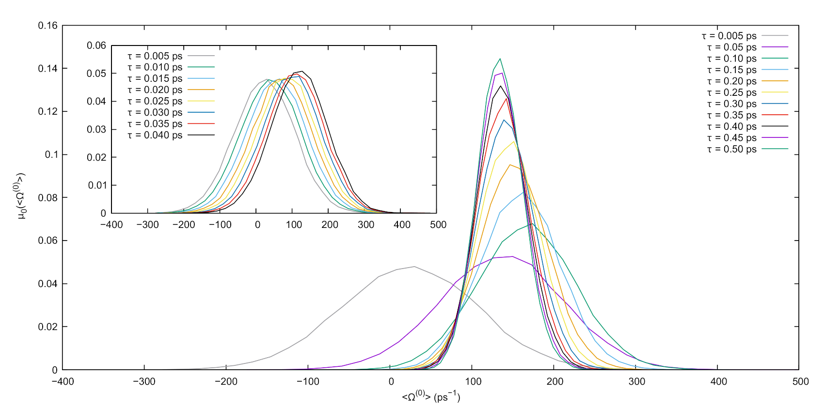The average dissipation function, Equation (10), is computed along each driven trajectory for a set of values of ${\tau }$, ranging from 5 to 500$\mathrm{fs}$. Probability distribution functions (PDFs) for the possible values of the average dissipation at different times are then extracted through a histogramming process. Results for the PDFs are presented in Figure 2, showing the typical shifting and narrowing around the driven value of the dissipation as the simulation time lengthens.

From the probabilities of opposite values of the average dissipation functions, it is possible to check Equation (11) for the system under investigation. Results are reported in Figure 3 for ${\tau }$ ranging from $0.015\mathrm{ps}$ to $0.115\mathrm{ps}$ together with the corresponding theoretical expectations, computed from Equation (11). As expected, the agreement between the theoretical result (solid curves) and the molecular dynamics calculation suffers as the length of the simulation and the value of A increase. The exponential behavior of the calculated quantities is, however, apparent and the agreement between the two sets of data is very good. To further quantify this agreement, in

Table 1. Comparison between the expected value of ${\tau }$ and the one obtained from the exponential fits performed on the numerical results in Figure 3.

${\mathit{\tau }}_{\mathbf{exp}}$ ($\mathbf{ps}$)	${\mathit{\tau }}_{\mathbf{simul}}$ ($\mathbf{ps}$)
$0.015$	$0.016\pm 0.001$
$0.025$	$0.026\pm 0.001$
$0.035$	$0.035\pm 0.001$
$0.045$	$0.044\pm 0.001$
$0.055$	$0.054\pm 0.001$
$0.065$	$0.063\pm 0.002$
$0.075$	$0.073\pm 0.002$
$0.085$	$0.086\pm 0.003$
$0.095$	$0.092\pm 0.003$
$0.105$	$0.103\pm 0.003$
$0.115$	$0.116\pm 0.005$

, we show the values for ${\tau }$ obtained from exponential fits performed on the numerical results and compare them with the exact value. In this case too, the agreement is very good within error bars.

4. Concluding Remarks

In this work, we have demonstrated that, and illustrated how, the transient FR can be actually verified in nonequilibrium molecular dynamics simulations of particles subject to magnetic and electric fields, and which are Nosé–Hoover thermostatted. The dissipation function, as well as the deterministic thermostat, have been expressed for the case in which electric and magnetic fields are parallel to each other. Although the applicability of generalized time-reversal symmetries implicitly implies the validity of the (transient) FR, based on the Nosé–Hoover canonical initial equilibrium distribution, the actual possibility of verifying it in a concrete, realistic simulation is not obvious. In the first place, to the best of our knowledge, this test has never been performed in presence of a magnetic field, which substantially modifies the dynamics of particles. In the second place, a verification of the FR may be hindered by the combination of scarce statistics and noise in the signal. Indeed, while the thermal noise becomes irrelevant at long observation (averaging) times, such long times drastically reduce the statistics of negative dissipations. Our simulations prove that the delicate balance allowing the verification of the FR, can be achieved for systems of moderately large size. Future developments will address the steady-state FR, which requires further conditions to be verified besides the time symmetry of the dynamics and of the initial phase-space probability distribution [13,28,36,37].

References

1. Landau, L.D.; Lifshitz, E. Statistical Physics; Elsevier: Amsterdam, The Netherlands, 1980. [Google Scholar]
2. de Groot, S.R.; Mazur, P. Non-Equilibrium Thermodynamics; Dover Publications: New York, NY, USA, 1984. [Google Scholar]
3. Barbier, M.; Gaspard, P. Microreversibility and nonequilibrium response theory in magnetic fields. J. Phys. A Math. Theor. 2018, 52, 025003. [Google Scholar] [CrossRef] [Green Version]
4. Casimir, H.B.G. On Onsager’s Principle of Microscopic Reversibility. Rev. Mod. Phys. 1945, 17, 343–350. [Google Scholar] [CrossRef] [Green Version]
5. Kubo, R. The fluctuation-dissipation theorem. Rep. Prog. Phys. 1966, 29, 255–284. [Google Scholar] [CrossRef] [Green Version]
6. Gaspard, P. Multivariate fluctuation relations for currents. New J. Phys. 2013, 15, 115014. [Google Scholar] [CrossRef]
7. Wang, C.; Feldman, D.E. Fluctuation theorems without time-reversal symmetry. Int. J. Mod. Phys. B 2014, 28, 1430003. [Google Scholar] [CrossRef] [Green Version]
8. Saito, K.; Utsumi, Y. Symmetry in Full Counting Statistics, Fluctuation Theorem, and Relations among Nonlinear Transport Coefficients in the Presence of a Magnetic Field. Phys. Rev. B 2008, 78, 115429. [Google Scholar] [CrossRef] [Green Version]
9. Evans, D.J.; Cohen, E.G.D.; Morriss, G.P. Probability of second law violations in shearing steady states. Phys. Rev. Lett. 1993, 71, 2401–2404. [Google Scholar] [CrossRef] [Green Version]
10. Gallavotti, G. Ergodicity, ensembles, irreversibility in Boltzmann and beyond. J. Stat. Phys. 1995, 78, 1571–1589. [Google Scholar] [CrossRef]
11. Evans, D.J.; Searles, D.J. The Fluctuation Theorem. Adv. Phys. 2002, 51, 1529–1585. [Google Scholar] [CrossRef]
12. Evans, D.J.; Searles, D.J.; Rondoni, L. Application of the Gallavotti-Cohen fluctuation relation to thermostated steady states near equilibrium. Phys. Rev. E 2005, 71, 056120. [Google Scholar] [CrossRef] [Green Version]
13. Rondoni, L.; Mejía-Monasterio, C. Fluctuations in nonequilibrium statistical mechanics: Models, mathematical theory, physical mechanisms. Nonlinearity 2007, 20, R1–R37. [Google Scholar] [CrossRef] [Green Version]
14. Roberts, J.; Quispel, G. Chaos and time-reversal symmetry. Order and chaos in reversible dynamical systems. Phys. Rep. 1992, 216, 63–177. [Google Scholar] [CrossRef]
15. Bonella, S.; Ciccotti, G.; Rondoni, L. Time reversal symmetry in time-dependent correlation functions for systems in a constant magnetic field. EPL Europhys. Lett. 2014, 108, 60004. [Google Scholar] [CrossRef]
16. Bonella, S.; Coretti, A.; Rondoni, L.; Ciccotti, G. Time-reversal symmetry for systems in a constant external magnetic field. Phys. Rev. E 2017, 96, 012160. [Google Scholar] [CrossRef] [PubMed]
17. Coretti, A.; Bonella, S.; Rondoni, L.; Ciccotti, G. Time reversal and symmetries of time correlation functions. Mol. Phys. 2018, 116, 3097–3103. [Google Scholar] [CrossRef]
18. Carbone, D.; Rondoni, L. Necessary and sufficient conditions for time reversal symmetry in presence of magnetic fields. Symmetry 2020, 12, 1336. [Google Scholar] [CrossRef]
19. Coretti, A.; Rondoni, L.; Bonella, S. Fluctuation Relations for Systems in a Constant Magnetic Field. Phys. Rev. E 2020, 102, 030101. [Google Scholar] [CrossRef]
20. Luo, R.; Benenti, G.; Casati, G.; Wang, J. Onsager reciprocal relations with broken time-reversal symmetry. Phys. Rev. Res. 2020, 2, 022009. [Google Scholar] [CrossRef] [Green Version]
21. Mouhat, F.; Bonella, S.; Pierleoni, C. Charge transport simulations of NaCl in an external magnetic field: The quest for the Hall effect. Mol. Phys. 2013, 111, 3651–3661. [Google Scholar] [CrossRef]
22. Jayannavar, A.M.; Sahoo, M. Charged particle in a magnetic field: Jarzynski equality. Phys. Rev. E 2007, 75, 032102. [Google Scholar] [CrossRef] [Green Version]
23. Poria, S.; Ghosh, S. Chaotic behavior of collective ion dynamics in the presence of an external static magnetic field. Phys. Plasmas 2016, 23, 062315. [Google Scholar] [CrossRef]
24. David, J.; José Casas-Vázquez, G.L. Extended Irreversible Thermodynamics; Springer: Berlin, Germany, 2010. [Google Scholar]
25. Morriss, G.P.; Rondoni, L. Definition of temperature in equilibrium and nonequilibrium systems. Phys. Rev. E 1999, 59, R5. [Google Scholar] [CrossRef] [Green Version]
26. Denis, J.E.; Morriss, G. Statistical Mechanics of Nonequilibrium Liquids; Cambridge University Press: Cambridge, UK, 2008. [Google Scholar]
27. Marconi, U.M.B.; Puglisi, A.; Rondoni, L.; Vulpiani, A. Fluctuation–dissipation: Response theory in statistical physics. Phys. Rep. 2008, 461, 111–195. [Google Scholar] [CrossRef] [Green Version]
28. Searles, D.J.; Rondoni, L.; Evans, D.J. The Steady State Fluctuation Relation for the Dissipation Function. J. Stat. Phys. 2007, 128, 1337–1363. [Google Scholar] [CrossRef] [Green Version]
29. Barbier, M.; Gaspard, P. Microreversibility, nonequilibrium current fluctuations, and response theory. J. Phys. A Math. Theor. 2018, 51, 355001. [Google Scholar] [CrossRef] [Green Version]
30. Tosi, M.P.; Fumi, G. Ionic Sizes and Born Repulsive Parameters in the NaCl-type Alkali Halides - II. J. Phys. Chem. Solids 1964, 25, 45–52. [Google Scholar] [CrossRef]
31. Ciccotti, G.; Jacucci, G. Direct Computation of Dynamical Response by Molecular Dynamics: The Mobility of a Charged Lennard-Jones Particle. Phys. Rev. Lett. 1975, 35, 789–792. [Google Scholar] [CrossRef]
32. Ciccotti, G.; Jacucci, G.; McDonald, I.R. Transport properties of molten alkali halides. Phys. Rev. A 1976, 13, 426–436. [Google Scholar] [CrossRef]
33. Mugnai, M.L.; Caprara, S.; Ciccotti, G.; Pierleoni, C.; Mareschal, M. Transient Hydrodynamical Behavior by Dynamical Nonequilibrium Molecular Dynamics: The Formation of Convective Cells. J. Chem. Phys. 2009, 131, 064106. [Google Scholar] [CrossRef]
34. Gagliardi, L.; Bonella, S. Charge transport in superionic and melted AgI under a magnetic field studied via molecular dynamics. Phys. Rev. B 2016, 94, 134426. [Google Scholar] [CrossRef]
35. Tuckerman, M. Statistical Mechanics: Theory and Molecular Simulation; Oxford University Press: Oxford, UK, 2010. [Google Scholar]
36. Searles, D.; Johnston, B.; Evans, D.; Rondoni, L. Time Reversibility, Correlation Decay and the Steady State Fluctuation Relation for Dissipation. Entropy 2013, 15, 1503–1515. [Google Scholar] [CrossRef] [Green Version]
37. Evans, D.J.; Williams, S.R.; Searles, D.J.; Rondoni, L. On Typicality in Nonequilibrium Steady States. J. Stat. Phys. 2016, 164, 842–857. [Google Scholar] [CrossRef] [Green Version]
38. Jepps, O.G.; Rondoni, L. Deterministic thermostats, theories of nonequilibrium systems and parallels with the ergodic condition. J. Phys. A Math. Theor. 2010, 43, 133001. [Google Scholar] [CrossRef]
39. Rondoni, L.; Verderosa, A. T-mixing: From fluctuation relations to response and irreversibility in MD. Mol. Simul. 2016, 42, 1135–1148. [Google Scholar] [CrossRef]
40. Adamo, P.; Belousov, R.; Rondoni, L. Fluctuation-Dissipation and Fluctuation Relations: From Equilibrium to Nonequilibrium and Back. In Large Deviations in Physics; Vulpiani, A., Cecconi, F., Cencini, M., Puglisi, A., Vergni, D., Eds.; Springer: Berlin/Heidelberg, Germany, 2014; Volume 885, pp. 93–133. [Google Scholar] [CrossRef]
Figure 1. Instantaneous dissipation function from Equation (8) for 500 fs of the “forward” evolution (red curve, open squares) and for 500 fs of the “backward” trajectory (blue curve, open triangles) obtained via M ext ( 3 ) (upper panel). The opposite values of the dissipation demonstrate the odd signature under the generalized time-reversal transformation used. The same behavior is not observed when the backward trajectory is obtained applying M s ext (bottom panel) as the presence of the magnetic field breaks the symmetry of the system under this transformation. Results are for the nonequilibrium simulation set-up described in Section 3 for liquid NaCl.
Entropy 23 00146 g001
Figure 2. Probability distribution functions estimated from the normalized histogram of the average dissipation function computed in nonequilibrium runs starting from 5 × 10 4 decorrelated equilibrium configurations for different values of τ . The main plot shows τ ranging from 0.005 to 0.5 ps , while the inset shows the trend for the low values of τ ranging from 0.005 to 0.04 ps , i.e., just after the switching on of the electric field that acts as the dissipative, nonequilibrium force.
Entropy 23 00146 g002
Figure 3. Simulation results for the transient fluctuation relation from the simulations described in Section 3. The points represent the ratio between probabilities (on the y-axis) of obtaining opposite values of the average dissipation (A, on the x-axis) at different values of τ from Figure 2. The statistical error is obtained dividing the 5 × 10 4 nonequilibrium runs in 50 blocks of 10 3 runs each and computing the normalized histogram for each of them. The error reported on the plot is obtained from the standard deviation on the single bin of the histograms relative to different blocks. Points are the simulation results, while the solid lines represent theoretical expectations. Parameters obtained from exponential fits performed on this set of numerical results are reported in Table 1. Note the logarithmic scale on the y-axis.
Entropy 23 00146 g003