
The Broadcast Approach in Communication Networks

.png)

Abstract
| Contents | ||
| 1 | Motivation and Overview | 4 |
| 1.1 What is the Broadcast Approach?................................................................................................................................................. | 4 | |
| 1.2 Degradedness and Superposition Coding........................................................................................................................................... | 5 | |
| 1.3 Application to Multimedia Communication......................................................................................................................................... | 6 | |
| 2 | Variable-to-Fixed Channel Coding | 7 |
| 2.1 Broadcast Approach in Wireless Channels......................................................................................................................................... | 7 | |
| 2.2 Relevance to the Broadcast Channel.............................................................................................................................................. | 8 | |
| 2.3 The SISO Broadcast Approach—Preliminaries..................................................................................................................................... | 9 | |
| 2.4 The MIMO Broadcast Approach..................................................................................................................................................... | 15 | |
| 2.4.1 Weak Supermajorization............................................................................................................................................ | 15 | |
| 2.4.2 Relation to Capacity.............................................................................................................................................. | 16 | |
| 2.4.3 The MIMO Broadcast Approach Derivation............................................................................................................................ | 17 | |
| 2.4.4 Degraded Message Sets............................................................................................................................................. | 19 | |
| 2.5 On Queuing and Multilayer Coding................................................................................................................................................ | 21 | |
| 2.5.1 Queue Model—Zero-Padding Queue.................................................................................................................................. | 22 | |
| 2.5.2 Delay Bounds for a Finite Level Code Layering..................................................................................................................... | 23 | |
| 2.5.3 Delay Bounds for Continuum Broadcasting........................................................................................................................... | 24 | |
| 2.6 Delay Constraints............................................................................................................................................................... | 27 | |
| 2.6.1 Mixed Delay Constraints........................................................................................................................................... | 27 | |
| 2.6.2 Broadcasting with Mixed Delay Constraints......................................................................................................................... | 28 | |
| 2.6.3 Parallel MIMO Two-State Fading Channel............................................................................................................................ | 30 | |
| 2.6.4 Capacity of Degraded Gaussian Broadcast Product Channels.......................................................................................................... | 31 | |
| 2.6.5 Extended Degraded Gaussian Broadcast Product Channels............................................................................................................. | 32 | |
| 2.6.6 Broadcast Encoding Scheme......................................................................................................................................... | 32 | |
| 2.7 Broadcast Approach via Dirty Paper Coding....................................................................................................................................... | 35 | |
| 3 | The Multiple Access Channel | 1 |
| 3.1 Overview........................................................................................................................................................................ | 35 | |
| 3.2 Network Model................................................................................................................................................................... | 35 | |
| 3.2.1 Discrete Channel Model............................................................................................................................................ | 37 | |
| 3.2.2 Continuous Channel Model.......................................................................................................................................... | 37 | |
| 3.3 Degradedness and Optimal Rate Spitting.......................................................................................................................................... | 38 | |
| 3.4 MAC without CSIT—Continuous Channels.......................................................................................................................................... | 38 | |
| 3.5 MAC without CSIT—Two-State Channels: Adapting Streams to the Single-User Channels............................................................................................. | 39 | |
| 3.6 MAC without CSIT—Two-State Channels: State-Dependent Layering................................................................................................................. | 40 | |
| 3.7 MAC without CSIT—Multi-State Channels: State-Dependent Layering............................................................................................................... | 45 | |
| 3.8 MAC with Local CSIT—Two-State Channels: Fixed Layering........................................................................................................................ | 47 | |
| 3.9 MAC with Local CSIT—Two-State Channels: State-Dependent Layering.............................................................................................................. | 48 | |
| 3.10 MAC with Local CSIT—Multi-State Channels: State-Dependent Layering............................................................................................................ | 51 | |
| 4 | The Interference Channel | 54 |
| 4.1 Overview........................................................................................................................................................................ | 54 | |
| 4.2 Broadcast Approach in the Interference Channel—Preliminaries.................................................................................................................. | 55 | |
| 4.3 Two-User Interference Channel without CSIT...................................................................................................................................... | 57 | |
| 4.3.1 Successive Decoding: Two-State Channel............................................................................................................................ | 58 | |
| 4.3.2 Successive Decoding: ℓ-State Channel............................................................................................................................ | 58 | |
| 4.3.3 Average Achievable Rate Region.................................................................................................................................... | 59 | |
| 4.3.4 Sum-Rate Gap Analysis............................................................................................................................................. | 61 | |
| 4.4 N-User Interference Channel without CSIT........................................................................................................................................ | 63 | |
| 4.5 Two-User Interference Channel with Partial CSIT................................................................................................................................. | 64 | |
| 4.5.1 Two-User Interference Channel with Partial CSIT—Scenario 1...................................................................................................... | 65 | |
| 4.5.2 Two-User Interference Channel with Partial CSIT—Scenario 2...................................................................................................... | 65 | |
| 5 | Relay Channels | 66 |
| 5.1 Overview........................................................................................................................................................................ | 66 | |
| 5.2 A Two-Hop Network............................................................................................................................................................... | 67 | |
| 5.2.1 Upper Bounds...................................................................................................................................................... | 68 | |
| 5.2.2 DF Strategies..................................................................................................................................................... | 70 | |
| 5.2.3 Continuous Broadcasting DF Strategies............................................................................................................................. | 71 | |
| 5.2.4 AF Relaying....................................................................................................................................................... | 75 | |
| 5.2.5 AQF Relay and Continuum Broadcasting.............................................................................................................................. | 76 | |
| 5.3 Cooperation Techniques of Two Co-Located Users.................................................................................................................................. | 78 | |
| 5.3.1 Lower and Upper Bounds............................................................................................................................................ | 80 | |
| 5.3.2 Naive AF Cooperation.............................................................................................................................................. | 82 | |
| 5.3.3 AF with Separate Preprocessing.................................................................................................................................... | 84 | |
| 5.3.4 Multi-Session AF with Separate Preprocessing...................................................................................................................... | 85 | |
| 5.3.5 Multi-Session Wyner–Ziv CF...................................................................................................................................... | 86 | |
| 5.4 Transmit Cooperation Techniques................................................................................................................................................. | 87 | |
| 5.4.1 Single-Layer Sequential Decode-and-Forward (SDF).................................................................................................................. | 88 | |
| 5.4.2 Continuous Broadcasting........................................................................................................................................... | 89 | |
| 5.4.3 Two Layer SDF—Successive Decoding............................................................................................................................... | 89 | |
| 5.5 Diamond Channel................................................................................................................................................................. | 92 | |
| 5.5.1 Decode-and-Forward................................................................................................................................................ | 92 | |
| 5.5.2 Amplify-and-Forward............................................................................................................................................... | 94 | |
| 5.6 Multi-Relay Networks............................................................................................................................................................ | 94 | |
| 5.6.1 Oblivious Relays.................................................................................................................................................. | 95 | |
| 5.6.2 Oblivious Agents.................................................................................................................................................. | 96 | |
| 5.7 Occasionally Available Relays................................................................................................................................................... | 97 | |
| 6 | Communications Networks | 98 |
| 6.1 Overview........................................................................................................................................................................ | 98 | |
| 6.2 Multi-User MAC Broadcasting with Linear Detection............................................................................................................................... | 98 | |
| 6.2.1 Channel Model..................................................................................................................................................... | 100 | |
| 6.2.2 Strongest Users Detection—Overview and Bounds................................................................................................................... | 100 | |
| 6.2.3 Broadcast Approach with Strongest Users Detection—(NO SIC)...................................................................................................... | 102 | |
| 6.2.4 SIC Broadcast Approach Upper Bound................................................................................................................................ | 103 | |
| 6.2.5 Broadcast Approach with Iterative SIC............................................................................................................................. | 104 | |
| 6.3 The Broadcast Approach for Source-Channel Coding................................................................................................................................ | 108 | |
| 6.3.1 SR with Finite Layer Coding....................................................................................................................................... | 109 | |
| 6.3.2 The Continuous SR-Broadcasting.................................................................................................................................... | 109 | |
| 6.4 The Information Bottleneck Channel.............................................................................................................................................. | 113 | |
| 6.4.1 Uncertainty of Bottleneck Capacity................................................................................................................................ | 115 | |
| 6.5 Transmitters with Energy Harvesting............................................................................................................................................. | 117 | |
| 6.5.1 Optimal Power Allocation Densities................................................................................................................................ | 119 | |
| 6.5.2 Optimal Power Allocation over Time................................................................................................................................ | 119 | |
| 6.5.3 Grouping the Constraints.......................................................................................................................................... | 120 | |
| 6.5.4 Dominant Constraints.............................................................................................................................................. | 121 | |
| 6.5.5 Optimality of Algorithm 1........................................................................................................................................ | 121 | |
| 7 | Outlook | 122 |
| A | Constants of Theorem 7 | 126 |
| B | Corner Points in Figure 16 | 127 |
| References | 128 | |
1. Motivation and Overview
1.1. What is the Broadcast Approach?
1.2. Degradedness and Superposition Coding
- 1.
- Degradedness in channel realizations: The first step in specifying a broadcast approach for a given channel pertains to designating a notion of degradedness that facilitates rank-ordering different realizations of a channel based on their relative strengths. The premise for assigning such degradedness is that if communication is successful in a specific realization, it will also be successful in all realizations considered stronger. For instance, in a single-user single-antenna wireless channel that undergoes a flat-fading process, the fading gain can be a natural degradedness metric. In this channel, as the channel gain increases, the channel becomes stronger. Adopting a proper degradedness metric hinges on the channel model. While it can emerge naturally for some channels (e.g., single-user flat-fading), in general, selecting a degradedness metric is rather heuristic, if possible at all. For instance, in the multiple access channel, the sum-rate capacity can be used as a metric to designate degradedness, while in the interference channel, comparing different network realizations, in general, is not well-defined.
- 2.
- Degradedness in message sets: Parallel to degradedness in channel realization, in some systems, we might have a natural notion of degradedness in the message sets as well. Specifically, in some communication scenarios (e.g., video communication), the messages can be naturally divided into multiple ordered layers that incrementally specify the entire message. In such systems, the first layer conveys the baseline information (e.g., the lowest quality version of a video); the second layer provides additional information that incrementally refines the baseline information (e.g., refining video quality), and so on. Such a message structure specifies a natural way of ordering the information layers, which should also be used by the receiver to retrieve the messages successfully. Specifically, the receiver starts by decoding the baseline (lowest-ranked) layer, followed by the second layer, and so on. While some messages have inherent degradedness structures (e.g., audio/video signals), that is not the case in general. When facing messages without an inherent degradedness structure, a transmitter can still split a message into multiple, independently generated information layers. The decoders, which are not constrained by decoding the layers in any specific order, will decode as many layers as they afford based on the actual channel realization.
- Degraded message sets. A message set with an inherent degradedness structure enforces a prescribed decoding order for the receiver.
- -
- Degraded channels. When there is a natural notion of degradedness among channel realizations (e.g., in the single-user single-antenna flat-fading channel), we can designate one message to each channel realization such that the messages are rank-ordered in the same way that their associated channels are ordered. At the receiver side, based on the actual realization of the channel, the receiver decodes the messages designated to the weaker channels, e.g., in the weakest channel realization, the receiver decodes only the lowest-ranked message, and in the second weakest realization, it decodes the two lowest-ranked messages, and so on. Communication over a parallel Gaussian channel is an example in which one might face degradedness both in the channel and the message [20].
- -
- General channels. When lacking a natural notion of channel degradedness (e.g., in the single-user multi-antenna channel or the interference channel), we generally adopt an effective (even though imperfect) approach to rank order channel realizations. These orders will be used to prescribe an order according to which the messages will be decoded. The broadcast approach in such settings mimics the Körner–Marton coding approach for broadcast transmission with degraded message sets [21]. This approach is known to be optimal for a two-user broadcast channel with a degraded set of messages, while the optimal strategy for the general broadcast approach is an open problem despite the significant recent advances, e.g., [22].
- General message sets. Without an inherent degradedness structure in the message, we have more freedom to generate the message set and associate the messages to different channel realizations. In general, each receiver has the freedom to decode any desired set of messages in any desired order. The single-user multi-antenna channel is an important example in which such an approach works effectively [23]. In this setting, while the channel is not degraded in general, different channel realizations are ordered based on the singular values of the channel matrix’s norm, which implies an order in channel capacities. In this setting, it is noteworthy that the specific choice of ordering the channels and assigning the set of messages decoded in each realization induces degradedness in the message set.
1.3. Application to Multimedia Communication
2. Variable-to-Fixed Channel Coding
2.1. Broadcast Approach in Wireless Channels
2.2. Relevance to the Broadcast Channel
2.3. The SISO Broadcast Approach—Preliminaries
2.4. The MIMO Broadcast Approach
2.4.1. Weak Supermajorization
2.4.2. Relation to Capacity
2.4.3. The MIMO Broadcast Approach Derivation
2.4.4. Degraded Message Sets
2.5. On Queuing and Multilayer Coding
2.5.1. Queue Model—Zero-Padding Queue
2.5.2. Delay Bounds for a Finite Level Code Layering
2.5.3. Delay Bounds for Continuum Broadcasting
- The number of layers is unlimited, that is .
- Since the layering is continuous, every layer i is associated with a fading gain parameter s. Every rate is associated with a differential rate specified in (3).
- The cumulative rate should be replaced by
- The sum is actually the average rate and it turns to be (7) for the continuum case.
2.6. Delay Constraints
2.6.1. Mixed Delay Constraints
2.6.2. Broadcasting with Mixed Delay Constraints
2.6.3. Parallel MIMO Two-State Fading Channel
2.6.4. Capacity of Degraded Gaussian Broadcast Product Channels
2.6.5. Extended Degraded Gaussian Broadcast Product Channels
2.6.6. Broadcast Encoding Scheme
2.7. Broadcast Approach via Dirty Paper Coding
3. The Multiple Access Channel
3.1. Overview
3.2. Network Model
3.2.1. Discrete Channel Model
3.2.2. Continuous Channel Model
3.3. Degradedness and Optimal Rate Spitting
3.4. MAC without CSIT—Continuous Channels
3.5. MAC without CSIT—Two-State Channels: Adapting Streams to the Single-User Channels
3.6. MAC without CSIT—Two-State Channels: State-Dependent Layering
- The second group of streams are reserved to be decoded in addition to when is strong, while is still weak.
- Alternatively, when is weak and is strong, instead the third group of streams, i.e., , are decoded.
- Finally, when both channels are strong, in addition to all the previous streams, the fourth group is also decoded.
3.7. MAC without CSIT—Multi-State Channels: State-Dependent Layering
3.8. MAC with Local CSIT—Two-State Channels: Fixed Layering
3.9. MAC with Local CSIT—Two-State Channels: State-Dependent Layering
- State-dependent Layering. In this approach, each transmitter, depending on the instantaneous state of the local CSI available to it, splits its message into independent information layers. Formally, when transmitter is in the weak state, it encodes its message by only one layer, which we denote by . On the other contrary, when transmitter is in the strong state, it divides its message into two information layers, which we denote by , and . Hence, transmitter i adapts the codebook (or ) to the state in which the other transmitter experiences a weak (or strong) channel. A summary of the layering scheme and the assignment of the codebooks to different network states is provided in Figure 14. In this table, the cell associated with the state for specifies the codebook adapted to this state.
- Decoding Scheme. A successive decoding scheme is designed based on the premise that as the combined channel state becomes stronger, more layers are decoded. Based on this, the total number of codebooks decoded increases as one of the two channels becomes stronger. In this decoding scheme, the combination of codebooks decoded in different states is as follows (and it is summarizes in Table 5):
- State : In this state, both transmitters experience weak states, and they generate codebooks according to Figure 14. In this state, the receiver jointly decodes the baseline layers and .
- State : When the channel of transmitter 1 is strong and the channel of transmitter 2 is weak, three codebooks are generated and transmitted. As specified by Table 5, the receiver jointly decodes . This is followed by decoding the remaining codebook, i.e., .
- State : In this state, codebook generation and decoding are similar to those in the state , except that the roles of transmitters 1 and 2 are interchanged.
- State : Finally, when both transmitters experience strong channels, the receiver decodes four codebooks in the order specified by the last row of Table 5. Specifically, the receiver first jointly decodes the baseline layers , followed by jointly decoding the remaining codebooks .
- Achievable Rate Region. Next, we provide an inner bound on the average capacity region. Recall that the average rate of transmitter i is denoted by , where the expectation is with respect to the random variables and . Hence, the average capacity region is the convex hull of all simultaneously achievable average rates . Furthermore, we define as the ratio of the total power P assigned to information layer , where we havefor all . The next theorem characterizes an average achievable rate region.
- Outer Bound. Next, we provide outer bounds on the average capacity region, and we compare them with the achievable rate region specified by Theorem 9.
- Outer bound 2: The second outer bound is the average capacity region of the two-user MAC with local CSI at transmitter 1 and full CSI at transmitter 2. Outer bound 2 is formally characterized in the following theorem.
3.10. MAC with Local CSIT—Multi-State Channels: State-Dependent Layering
- State : Start with the weakest channel combination , and reserve the baseline codebooks to be the only codebooks to be decoded in this state. Define as the set of codebooks that the receiver decodes from transmitter i when the channel state is .
- States and : Next, construct the first row of the table. For this purpose, define as the set of the codebooks that the receiver decodes from transmitter 2, when the channel state is . Based on this, the set of codebooks in each state can be specified recursively. Specifically, in the state , decode what has been decoded in the preceding state , i.e., the set of codebooks , plus new codebooks . Then, construct the first column of the table in a similar fashion, except that the roles of transmitter 1 and 2 are swapped.
- States for : By defining the set of codebooks that the receiver decodes from transmitter i in the state by , the codebooks decoded in this state are related to the ones decoded in two preceding states. Specifically, in state decode codebooks and . For example, for , the codebooks decoded in include those decoded for transmitter 1 in state along with those decoded for transmitter 2 in channel state .
4. The Interference Channel
4.1. Overview
4.2. Broadcast Approach in the Interference Channel—Preliminaries
4.3. Two-User Interference Channel without CSIT
- Transmitter 1 (or 2) reserves the information layer (or ) for adapting it to the channel from transmitter 1 (or 2) to the unintended receiver (or ). Based on this designation, the intended receivers (or ) will decode all codebooks (or ), and the non-intended receivers (or ) will be decoding a subset of these codebooks. The selection of the subsets depends on on channel strengths of the receivers, such that the non-intended receiver (or ) decodes only codebooks (or ).
- Transmitter 1 (or 2) reserves the layer (or ) for adapting it to the channel from transmitter 2 (or 1) to the intended receiver (or ). Based on this designation, the unintended receivers (or ) will not decode any of the codebooks (or ), and the intended receivers (or ) will be decoding a subset of these codebooks. The selection of these subsets depends on channel strengths of the receives such that the intended receiver (or ) decodes only the codebooks (or ).
4.3.1. Successive Decoding: Two-State Channel
4.3.2. Successive Decoding: ℓ-State Channel
- Receiver 1—stage 1 (Codebooks ): Receiver 1 decodes one information layer from each transmitter in an alternating manner until all codebooks and are decoded. The first layer to be decoded in this stage depends on the state . If , the receiver starts by decoding codebook from transmitter 1, then it decodes the respective layer from transmitter 2, and continues alternating between the two transmitters. Otherwise, if , receiver 1 first decodes from the interfering transmitter 2, followed by from transmitter 1, and continues alternating. By the end of stage 1, receiver 1 has decoded q codebooks from each transmitter.
- Receiver 1—stage 2 (Codebooks and ): In stage 2, receiver 1 carries on decoding layers from transmitter 1, in an ascending order of the index s. Finally, receiver 1 decodes layers specially adapted to receivers , in an ascending order of index s. Throughout stage 2, receiver 1 has additionally decoded K codebooks from its intended transmitter 1.
4.3.3. Average Achievable Rate Region
4.3.4. Sum-Rate Gap Analysis
- Weak interference: In the weak interference regime, the capacity with full CSIT is in unknown. In this regime, in order to quantify the gap of interest, we first evaluate the gap of the sum-rate achieved by the scheme of Section 4.3.2 to the sum-rate achieved by the HK scheme. By using this gap in conjunction with the known results on the gap between the sum-rate of HK and the sum-rate capacity, we provide an upper bound on the average sum-rate gap of interest.
- Strong interference: In the strong interference regime, the sum-rate capacity with full CSIT is known. It can be characterized by evaluating the sum-rate of the intersection of two capacity regions corresponding to two multiple access channels formed by the transmitters and each of the receivers [123].
- (i)
- For we have
- (ii)
- For we have
4.4. N-User Interference Channel without CSIT
- Transmitter m adapts layer to the state of the channels linking all other transmitters to the unintended receivers : while the intended receivers will be decoding all codebooks , the non-intended receivers decode a subset of these codebooks depending on their channel strengths. More specifically, a non-intended receiver decodes only the codebooks .
- Transmitter m adapts the layer to the state of the channels linking all other transmitters to the intended receiver : while the unintended receivers will not be decoding any of the codebooks , the intended receivers decode a subset of these codebooks depending on their channel strengths. More specifically, the intended receiver decodes only the codebooks .
4.5. Two-User Interference Channel with Partial CSIT
4.5.1. Two-User Interference Channel with Partial CSIT—Scenario 1
- State-dependent adaptive layering. In this setting, each transmitter controls the interference that it imposes by leveraging the partially known CSI. Concurrently, each transmitter adapts one layer to every possible channel state at its intended receiver, overcoming the partial uncertainty about the other transmitter’s interfering link. Based on these observations, transmitter i splits its information stream into a certain set of codebooks depending on the state of its outgoing cross channel. We denote the set of codebooks transmitted by user i when by . Each set consists of codebooks given by
- layer () is adapted to the cross channel state at the unintended receiver (); and
- layer ( ) is adapted to the cross channel state at the intended receiver (), for .
- Successive decoding. Each codebook will be decoded by multiple receivers in the equivalent network formed by different receivers associated with different network states. Hence, each codebook rate will be constrained by its associated most degraded channel state. Furthermore, any undecoded layer at a particular receiver imposes interference, which degrades the achievable rate at that receiver. Motivated by these premises, a simple successive decoding scheme can be designed that specifies (i) the set of receivers at which each layer is decoded, and (ii) the order of successive decoding order at each receiver.
- Receiver : First, it decodes one layer from the unintended transmitter and remove it from the received signal. Secondly, it decodes the baseline layer from its intended transmitter . Finally, depending on the network state , it successively decodes all the layers .
- Receiver : First, it decodes one layer from the unintended transmitter and remove it from the received signal. Secondly, it decodes the baseline layer from its intended transmitter . Finally, depending on the network state , it successively decodes all the layers .
4.5.2. Two-User Interference Channel with Partial CSIT—Scenario 2
- State-dependent adaptive layering. In contrast to Scenario 1, in this scenario, transmitter i knows , and it is oblivious to the other channel. Lacking the extent of interference that each transmitter causes, transmitter i adapts multiple layers with different rates such that the unintended receiver opportunistically decodes and removes a part of the interfering according to the actual state of the channel. Simultaneously, transmitter i adapts the encoding rate of a single layer to be decoded only by its intended receiver based on the actual state of channel . Based on this vision, transmitter i splits its information stream into a distinct set of codebooks corresponding to each state of the cross channel at its intended receiver. We denote the set of codebooks transmitted by user i when by . Each set consists of codebooks given by
- layer () is adapted to the cross channel state at the unintended receiver (), for ; and
- layer () is adapted to the cross channel state at the intended receiver ().
- Successive decoding. Given that each codebook will opportunistically be decoded by multiple receivers, its maximum achievable rate is constrained by the most degraded network state in which it is decoded. Similarly to that of Scenario 1, a successive decoding scheme is devised that specifies (i) the set of receivers at which each layer is decoded, and (ii) the order of successive decoding order at each receiver.
- Receiver : First, it decodes one layer from the interfering signal . Afterwards, it decodes one layer from the intended signal . This receiver continues the decoding process in an alternating manner until codebooks from transmitter 2 and codebooks are decoded from the intended receiver 1 are successfully decoded. Finally, the last remaining layer from the intended message is decoded.
- Receiver : First, it decodes one layer from the interfering signal . Afterwards, it decodes one layer from the intended signal . This receiver continues the decoding process in an alternating manner until codebooks from transmitter 1 and codebooks are decoded from the intended receiver 2 are successfully decoded. Lastly, the last remaining layer from the intended message is decoded.
5. Relay Channels
5.1. Overview
5.2. A Two-Hop Network
5.2.1. Upper Bounds
5.2.2. DF Strategies
5.2.3. Continuous Broadcasting DF Strategies
- Coding Scheme I—Source: Outage and Relay: Continuum Broadcasting. In this coding scheme, the source transmitter performs single-level coding. Whenever channel conditions allow decoding at the relay, it performs continuum broadcasting, as described in the previous subsection. Thus, the received rate at the destination depends on the instantaneous channel fading gain realization on the relay-destination link. Clearly, a necessary condition for receiving something at the destination is that channel conditions on the source-relay link will allow decoding. The source transmission rate is given by
- Coding Scheme II—Source: Continuum Broadcasting and Relay: Outage. In this coding scheme, the source transmitter performs continuum broadcasting, as described in the previous subsection. The relay encodes the successfully decoded layers into a single-level block code. Thus, the rate of each transmission from the relay depends on the number of layers decoded. For a fading gain realization on the source-relay link, the decodable rate at the relay is
- Coding Scheme III—Source and Relay: Continuous Broadcasting. In this scheme, both source and relay perform the optimal continuum broadcasting. The source transmitter encodes a continuum of layered codes. The relay decodes up to the maximal decodable layer. Then it retransmits the data in a continuum multi-layer code matched to the rate that has been decoded last. In this scheme, the source encoder has a single power distribution function, which depends only on a single fading gain parameter. The relay uses a power distribution that depends on the two fading gains on the source-relay and the relay-destination links.
5.2.4. AF Relaying
5.2.5. AQF Relay and Continuum Broadcasting
5.3. Cooperation Techniques of Two Co-Located Users
- Naive AF—A helping node scales its input and relays it to the destined user, who jointly decodes the relay signal and the direct link signal.
- Separate preprocessing AF—A more efficient form of single-session AF is a separate preprocessing approach in which the co-located users exchange the values of the estimated fading gains, and each individually decodes the layers up to the smallest fading gain. The helping user removes the decoded common information from its received signal and performs AF on the residual signal to the destined user.
- Multi-session AF—Repeatedly separate preprocessing is followed by a transmitting cooperation information at both helper and destination nodes (on orthogonal channels). The preprocessing stage includes individual decoding of the received information from the direct link and previous cooperation sessions. Along the cooperation sessions, transmission of the next block already takes place. It means that multi-session cooperation introduces additional decoding delays without any impact on the throughput. For this purpose, multiple parallel cooperation channels are assumed. For incorporating practical constraints on the multi-session approach, the total power of multi-session cooperation is restricted to . This is identical to the power constraint in single-session cooperation.
- Naive CF—A helping node performs WZ-CF over the cooperation link. The destination informs the relay of its fading gain realization prior to the WZ compression. The destination performs optimal joint decoding of the WZ compressed signal forwarded over the cooperation link, and its own copy of the signal from the direct link.
- Separate preprocessing CF—Each user decodes independently up to the highest common decodable layer. Then WZ–CF cooperation takes place on the residual signal by WZ coding.
- Multi-session CF— Multi-session cooperation, as described for AF, is carried out in conjunction with successive refinement WZ [193] CF relaying.
5.3.1. Lower and Upper Bounds
- Outage lower bound. The single-layer coding expected rate is
- Broadcasting lower bound. This bound is based on an SISO block fading channel, with receive CSI. The maximal expected broadcasting rate [23], for a Rayleigh fading channel is
- Ergodic lower bound. Ergodic capacity of a general SIMO channel with m receiver antennas is [66]
- Ergodic upper bound. Ergodic bound for two receive antennas SIMO fading channel is in (313),
- Single-session cut-set upper bound. Another upper bound considered is the classical cut-set bound of the relay channel [40]. This bound may be useful for single-session cooperation, where the capacity of the cooperation link is rather small. Using the relay channel definitions in (306) and (307), and assuming a single cooperation session , the cut-set bound for a Rayleigh fading channel is given by
5.3.2. Naive AF Cooperation
5.3.3. AF with Separate Preprocessing
5.3.4. Multi-Session AF with Separate Preprocessing
5.3.5. Multi-Session Wyner–Ziv CF
5.4. Transmit Cooperation Techniques
5.4.1. Single-Layer Sequential Decode-and-Forward (SDF)
5.4.2. Continuous Broadcasting
5.4.3. Two Layer SDF—Successive Decoding
5.5. Diamond Channel
5.5.1. Decode-and-Forward
5.5.2. Amplify-and-Forward
5.6. Multi-Relay Networks
5.6.1. Oblivious Relays
5.6.2. Oblivious Agents
5.7. Occasionally Available Relays
6. Communications Networks
6.1. Overview
6.2. Multi-User MAC Broadcasting with Linear Detection
- formulation of ergodic bounds for systems with random spreading DS-CDMA over fading channels, employing SIC receivers;
- derivation of the expected spectral efficiency achievable with equal rate allocation per user, and iterative SIC decoding. It is also shown that equal rate allocation maximizes the expected spectral efficiency;
- derivation of the expected spectral efficiency for the case of multi-layer coding taken to the limit of many layers (continuous broadcast approach);
- analysis of a multi-layer coding where parallel decoders are used, without employing SIC;
- analysis of a more complicated setting, including a multi-layer coded transmission with iterative SIC decoding. It is shown that, like in the single-layer case, the expected spectral efficiency is maximized for equal rate allocation per user. Furthermore, the optimal layering power allocation function, which maximizes the expected spectral efficiency, is obtained for the matched-filter and decorrelator detectors. The case of broadcasting with MMSE and optimal detectors under iterative SIC decoding remains an open problem.
6.2.1. Channel Model
6.2.2. Strongest Users Detection—Overview and Bounds
- Upper bound. It is well-known that the optimum multiuser detector capacity is also equal to the ergodic successive decoding sum-rate capacity with an MMSE detector, according to the mutual information chain rule [40]. Thus the ergodic capacity, obtained with an optimum detector, can be expressed by the ergodic SIC MMSE detection capacity [217]
- Strongest users detection. It refers to the practical case where all users transmit at a fixed rate, via single-layer coding. The adequate channel model here is the block fading channel, where a fixed fading realization throughout the block for each user is observed. Thus, all users experiencing fading gains smaller than a threshold will not be reliably decoded. This is demonstrated in Figure 31, where a fraction of users, corresponding to , is in an outage, and all other users are reliably decoded. The average achievable sum-rate for outage decoding is given by [218]
6.2.3. Broadcast Approach with Strongest Users Detection—(NO SIC)
6.2.4. SIC Broadcast Approach Upper Bound
6.2.5. Broadcast Approach with Iterative SIC
6.3. The Broadcast Approach for Source-Channel Coding
6.3.1. SR with Finite Layer Coding
6.3.2. The Continuous SR-Broadcasting
6.4. The Information Bottleneck Channel
6.4.1. Uncertainty of Bottleneck Capacity
6.5. Transmitters with Energy Harvesting
6.5.1. Optimal Power Allocation Densities
6.5.2. Optimal Power Allocation over Time
6.5.3. Grouping the Constraints
| Algorithm 1. Computing . |
1: set according to (489) . 2: initialize and , 3: while 4: 5: set 6: for 7: set as the solution to 8: set 9: end for 10: (if not unique select the smallest) 11: 12: 13: end while 14: for 15: for 16: 17: end for 18: end for |
6.5.4. Dominant Constraints
6.5.5. Optimality of Algorithm 1
7. Outlook
- Single-user MIMO channel. Designing an optimal broadcast approach for the general MIMO channel is still an open problem since the MIMO channel is a non-degraded broadcast channel [68,69]. Its capacity region is known for multiple users with private messages [50], and for two users with a common message [67]. However, a complete characterization of the broadcast approach requires the full solution of the most general MIMO broadcast channel with a degraded message set [21], which is not yet available (infinite number of realizations, for H with Gaussian components), and hence suboptimal ranking procedures were considered. Various degraded message sets and transmission schemes with sub-optimal ranking at the receiver are studied in [23,70,71]. Formulation of the general MIMO broadcasting with degraded message sets and the optimization of the layering power distribution, which maximizes the expected rate, is stated in (71) and (73). This optimization problem does not lend itself to a closed-form solution and remains an open problem for future research. The framework analyzed in [239], which uses rate-splitting and binning, may be useful for the general broadcast problem with degraded message sets. It is shown in [240] that a tight upper bound might be obtained for the two users broadcast channel by adding an auxiliary receiver. Generalizing this work for multiple users may provide an efficient tool for obtaining outer bounds in general and on the MIMO broadcast approach.
- Binary-dirty paper coding. DPC has a pivotal role in Gaussian broadcast transmissions. Owing to its optimality for some settings (e.g., MIMO broadcast channel [50]), an interesting research direction is investigating the performance or operation gains (e.g., rate and latency) of using DPC instead of superposition coding in the settings discussed in Section 2 and Section 6. From a broader perspective, binning techniques facilitate DPC to be effective beyond Gaussian channels. In particular, Marton’s general capacity region relies on the basic elements of binning [244], in the context of which the classical Gelfand–Pinsker [245] strategy can be interpreted as a vertex point [245]. The Gelfand–Pinsker strategy in the Gaussian domain becomes DPC [91,245]. The study in [246] addresses both binning and superposition coding aspects in a unified framework. Furthermore, this study also investigates mismatched decoding, which can account for the imperfect availability of the CSI at the receivers. It is also noteworthy that throughout the paper, we primarily focused on the notion of physically degraded channels and rank-ordering them based on their degradedness. Nevertheless, it is important to investigate less restrictive settings, such as less-noisy channels [94,247,248].
- Secrecy. When considering the broadcast approach, it is natural to look also at secrecy in communications. Such an approach not only involves determining which decoded messages depend on the channel state, but it also involves determining those that are required to be kept secret [201,202,209,249]. This can be designed as part of the multi-layer broadcast approach.
- Latency. There are various aspects in which delay constraints in communications may impact the system design, some of which were discussed in Section 2. There exists significant room for incorporating fixed-to-variable channel coding and variable-to-variable channel coding in the broadcast approach. In a way, this is a combination of variable-to-fixed coding (broadcast approach) and fixed-to-variable coding (that is, Fountain-like schemes). For example, some applications allow decoding following multiple independent transmission blocks, as considered in [87], and studied by its equivalent channel setting, which is the MIMO parallel channel [20]. Queuing theory can be used to analyze the expected achievable latency, as in [80]. An interesting observation is that layering often offers higher latency gains than throughput gains. The problem of resource allocation for delay minimization, even under a simple queue model as in [80], remains an open problem for further research. Similarly, a generalization of the queue model with parallel queues associated with multiple streams, each with a different arrival random process and a different delay constraint, is an important direction to investigate.
- Connection to I-MMSE. It is well-known that the scalar additive Gaussian noise channel has the single crossing point property between the MMSE in the estimate of the input given the channel output. This property also provides an alternative proof to the capacity region of the scalar two-user Gaussian broadcast channel [250]. This observation is extended to the vector Gaussian channel [71] via information-theoretic properties on the mutual information, using the I-MMSE relationship, a fundamental connection between estimation theory and information theory shown in [250]. An interesting future direction is investigating the impact of I-MMSE relation on the broadcast approach.
- Information bottleneck. Another interesting setting is the information bottleneck channel. In this channel model, a wireless block fading channel is connected to a reliable channel with limited capacity, referred to as the bottleneck channel [198,199]. In these studies, it is assumed that the transmitted signal is Gaussian, which made it possible to describe the optimal continuous layering power distribution in closed-form expressions. Extensions beyond Gaussian have both practical and theoretical significance.
- Implementation. The actual implementation of the broadcast approach, in general, is a rich topic for further research. Evidently, as it is mainly associated with layered decoding, this can be done by a variety of advanced coding and modulation techniques such as the low-density parity-check (LDPC) codes and turbo codes. The work in [260] considers LDPC implementation in conjunction with rate-splitting (no CSIT) in the interference channel, and [261] provides bounds on LDPC codes over an erasure channel with variable erasures. Polar codes can be directly adopted for implementing the broadcast approach as their decoding is based on successive cancellations, and hence they naturally fit in the broadcast approach. Its efficiency has been demonstrated in the general broadcast channel [262,263], and further its ability to work on general channels without adapting the transmitter to the actual channel [264] demonstrates the special features that are central to the broadcast approach. Furthermore, its applicability to multiple description [265] make it a natural candidate that can be used for implementing joint source-channel coding via a broadcast approach. Polar codes may also be used to practically address the variable-to-variable rate channel coding, as it is suitable for variable-to-fixed channel coding as well as fixed-to-variable channel coding, as demonstrated in [266] for rateless codes. Power allocation across different information layers in special cases is investigated in [267], and there is room for further generalizing the results.
- Finite blocklength. This paper focuses primarily on the asymptotically long transmission blocks. It is also essential to analyze the broadcast approach in the non-asymptotic block length regime. In such regimes, one could compromise the distribution of rates (asymptotic regime) with second-order descriptions, or even random coding error exponents, as there is a tradeoff between the error exponent rate of a finite block and the maximum rate. The practical aspects of communication under stringent finite blocklength constraints are discussed in [268].
- Identification via channels. The identification problem introduced in [269] is another case of a state-dependent channel. Its objective is communicating messages over a channel to select a group of messages at the receiver. This is in contrast to Shannon’s formulation in which the objective is selecting one message. Many of the challenges pertinent to state-dependent channels and the lack of CSIT that appear in Shannon’s formulation are relevant for the identification problem as well. Recent studies on the identification via channels without the CSIT include [270].
- Mixed-delay constraints. One major challenge in modern communication systems is heterogeneity in data type and their different attendant constraints. One such constraint pertains to latency, where different data types and streams can face various delay constraints. The broadcast approach investigated for addressing mixed-delay constraints in the single-user channel [84], can be further extended to address this problem in more complex settings (e.g., soft handoff in cellular systems [86] and C-RAN uplink [85]) while facing the lack of CSIT and in the context of fixed-to-variable channel coding [6] and fountain codes [271].
- Source coding. Another application is source coding with successive refinement where side information at the receiver (Wyner–Ziv) can be different, e.g., another communications link that might provide information and its quality is not known at the transmitter [272]. Another possible extension is the combination of successive refinements and broadcast approach [32].
- Caching. In cooperative communication, it is common that relay stations perform data caching [273,274], and the transmitter has no information about what is being cached. This random aspect of the amount and location (for multi-users) of cashing might play an interesting role in a broadcast approach for such a system.
- Algebraic structured codes. The information-theoretic analyses of the networks reviewed in this paper generally are based on unstructured code design. In parallel to unstructured codes, there is rich literature on the structured design of codes with a wide range of applications to multi-terminal communication (e.g., multiple access and interference channels) and distributed source coding. A thorough recent overview of algebraic codes is available in [275].
- Networking. All different settings and scenarios discussed in this article play important roles in communication networks. As a network’s size and complexity grow, the users cannot be all provided with the complete and instantaneous state of the networks. Specifically, in the future wireless systems (e.g., 6G), cell-based hierarchical network architectures will be dispensed with [276]. In such networks, acquiring the CSI at the transmitters will be impossible, in which case the broadcast approach will be effective in circumventing the lack of CSIT. Furthermore, network coding can be incorporated in the broadcast approach, as it can account for latency, general wireless impediments (e.g., fading), and various network models, e.g., the relay, broadcast, interference, and multiple-access channels [277].Finally, we highlight that the broadcast approach’s hallmark is that it enables communication systems to adapt their key communication performance metrics (e.g., data rate, service latency, and message distortion) to the actual realizations of the communication channels. Such a feature is especially important as the size, scale, and complexity of the communication systems grow, rendering the instantaneous acquisition of channel realizations at the transmitters costly, if not prohibitive altogether. Adapting communication to unknown channels is an inherent property of communication systems in the pre-digital (analog) era, facilitating the mainstream adoption of broadcasting technologies for distributing audio and video contents. The broadcast technology instates this property in digital communication systems as well.
Author Contributions
Funding
Conflicts of Interest
Abbreviations
| AF | amplify-and-forward |
| AQF | hybrid amplify-quantize-and-forward |
| AWGN | additive white Gaussian noise |
| BCC | broadcasting coherent combining |
| BIR | broadcasting incremental redundancy |
| CC | coherent combining |
| CDF | cumulative distribution function |
| CDMA | code-division multiple access |
| CF | compress-and-forward |
| CSI | channel state information |
| CSIT | channels state information at the transmitter sites |
| DC | delay constrained |
| DF | decode-and-forward |
| DoF | Degrees-of-freedom |
| DS | direct-sequence |
| DSL | digital subscriber line |
| FCSI | full CSI |
| FUU | fraction of undecodable users |
| HARQ | hybrid automatic retransmission request |
| HK | Han–Kobayashi |
| IR | incremental redundancy |
| LTSC | Long-term static channel |
| MAC | multi-access channel |
| MF | matched filter |
| MIMO | multiple input multiple output |
| MISO | multiple input single output |
| MLC | multi-level coding |
| MMSE | minimum mean squared-error |
| NDC | non-delay constrained |
| OAR | outage approach retransmission |
| probability distribution function | |
| PET | priority encoding transmission |
| QF | quantize-and-forward |
| RV | random variable |
| SDF | sequential decode and forward |
| SIC | successive interference cancellation |
| SINR | signal to interference and noise ratio |
| SISO | single input single output |
| SIMO | single input multiple output |
| SNR | signal-to-noise ratio |
| SR | successive refinement |
Appendix A. Constants of Theorem 7
Appendix B. Corner Points in Figure 16
References
- Burnashev, M.V. Data transmission over discrete channel with feedback: Random transmission time. Probl. Peredachi Inf. 1976, 12, 10–30. [Google Scholar]
- Tchamkerten, A.; Telatar, E. Variable length coding over an unknown channel. IEEE Trans. Inf. Theory 2006, 52, 2126–2145. [Google Scholar] [CrossRef]
- Shayevitz, O.; Feder, M. Achieving the empirical capacity using feedback: Memoryless additive models. IEEE Trans. Inf. Theory 2009, 55, 1269–1295. [Google Scholar] [CrossRef]
- Polyanskiy, Y.; Poor, H.V.; Verdú, S. Variable-length coding with feedback in the non-asymptotic regime. In Proceedings of the IEEE International Symposium on Information Theory, Austin, TX, USA, 13–18 June 2010. [Google Scholar]
- Tyagi, H.; Narayan, P. State-dependent channels: Strong converse and bounds on reliability function. In Excursions in Harmonic Analysis; Springer: Cambridge, MA, USA, 2013. [Google Scholar]
- Verdú, S.; Shamai (Shitz), S. Variable-rate channel capacity. IEEE Trans. Inf. Theory 2010, 56, 2651–2667. [Google Scholar] [CrossRef]
- Biglieri, E.; Proakis, J.; Shamai (Shitz), S. Fading channels: Information-theoretic and communication aspects. IEEE Trans. Inf. Theory 1998, 44, 2619–2692. [Google Scholar] [CrossRef]
- Shamai (Shitz), S.; Telatar, E. Some information-theoretic aspects of decentralized power control in multiple access fading channels. In Proceedings of the Information Theory and Networking Workshop, Metsovo, Greece, 27 June–1 July 1999. [Google Scholar]
- Sharif, M.; Hassibi, B. Delay considerations for opportunistic scheduling in broadcast fading channels. IEEE Trans. Wirel. Commun. 2007, 6, 3353–3363. [Google Scholar] [CrossRef]
- Asadi, A.; Mancuso, V. A survey on opportunistic scheduling in wireless communications. IEEE Commun. Surv. Tutor. 2013, 15, 1671–1688. [Google Scholar] [CrossRef]
- Zhao, Q.; Sadler, B.M. A survey of dynamic spectrum access. IEEE Signal Process. Mag. 2007, 24, 79–89. [Google Scholar] [CrossRef]
- Tanab, M.E.; Hamouda, W. Resource allocation for underlay cognitive radio networks: A survey. IEEE Commun. Surv. Tutor. 2016, 19, 1249–1276. [Google Scholar] [CrossRef]
- Ozarow, L.; Shamai (Shitz), S.; Wyner, A. Information-theoretic considerations for cellular mobile radio. IEEE Trans. Veh. Technol. 1994, 43, 359–378. [Google Scholar] [CrossRef]
- Hanly, S.V.; Tse, D.N.C. Multiaccess fading channels—Part II: Delay-limited capacities. IEEE Trans. Inf. Theory 1998, 44, 2816–2831. [Google Scholar] [CrossRef]
- Li, L.; Jindal, N.; Goldsmith, A. Outage capacities and optimal power allocation for fading multiple-access channels. IEEE Trans. Inf. Theory 2005, 51, 1326–1347. [Google Scholar] [CrossRef]
- Narasimhan, R. Individual outage rate regions for fading multiple access channels. In Proceedings of the IEEE International Symposium on Information Theory, Nice, France, 24–29 June 2007; pp. 1571–1575. [Google Scholar]
- Haghi, A.; Khosravi-Farsani, R.; Aref, M.; Marvasti, F. The capacity region of fading multiple access channels with cooperative encoders and partial CSIT. In Proceedings of the IEEE International Symposium on Information Theory, Austin, TX, USA, 13–18 June 2010; pp. 485–489. [Google Scholar]
- Das, A.; Narayan, P. Capacities of time-varying multiple-access channels with side information. IEEE Trans. Inf. Theory 2001, 48, 4–25. [Google Scholar] [CrossRef]
- Jafar, S. Capacity with causal and noncausal side information: A unified view. IEEE Trans. Inf. Theory 2006, 52, 5468–5474. [Google Scholar] [CrossRef]
- Cohen, K.M.; Steiner, A.; Shamai (Shitz), S. On the broadcast approach over parallel MIMO two-state fading channel. In Proceedings of the IEEE International Zurich Seminar on Information and Communication, Zurich, Switzerland, 26–28 February 2020. [Google Scholar]
- Körner, J.; Marton, K. General broadcast channels with degraded message sets. IEEE Trans. Inf. Theory 1977, 23, 60–64. [Google Scholar] [CrossRef]
- Nair, C.; El Gamal, A. The capacity region of a class of three-receiver broadcast channels with degraded message sets. IEEE Trans. Inf. Theory 2009, 55, 4479–4493. [Google Scholar] [CrossRef]
- Shamai (Shitz), S.; Steiner, A. A broadcast approach for a single-user slowly fading MIMO channel. IEEE Trans. Inf. Theory 2003, 49, 2617–2635. [Google Scholar] [CrossRef]
- Cover, T.M. Broadcast channels. IEEE Trans. Inf. Theory 1972, 18, 2–14. [Google Scholar] [CrossRef]
- Shamai (Shitz), S. A broadcast strategy for the Gaussian slowly fading channel. In Proceedings of the IEEE International Symposium on Information Theory, Ulm, Germany, 29 June–4 July 1997; p. 150. [Google Scholar]
- Berger, T.; Gibson, J.D. Lossy source coding. IEEE Trans. Inf. Theory 1998, 44, 2693–2723. [Google Scholar] [CrossRef]
- Wolf, J.K.; Wyner, A.D.; Ziv, J. Source coding for multiple descriptions. Bell Syst. Tech. J. 1980, 59, 1417–1426. [Google Scholar] [CrossRef]
- Steiner, A.; Shamai (Shitz), S. The broadcast approach in communications systems. In Proceedings of the IEEE Convention of Electrical and Electronics Engineers in Israel, Eilat, Israel, 3–5 December 2008. [Google Scholar]
- Equitz, W.H.R.; Cover, T.M. Successive refinement of information. IEEE Trans. Inf. Theory 1991, 37, 269–275. [Google Scholar] [CrossRef]
- Rimoldi, B. Successive refinement of information: Characterization of the achievable rates. IEEE Trans. Inf. Theory 1994, 40, 253–259. [Google Scholar] [CrossRef]
- Ng, C.T.K.; Tian, C.; Goldsmith, A.J.; Shamai (Shitz), S. Minimum expected distortion in Gaussian source coding with uncertain side information. In Proceedings of the IEEE Information Theory Workshop, Solstrand, Norway, 1–6 July 2007; pp. 454–459. [Google Scholar]
- Tian, C.; Steiner, A.; Shamai (Shitz), S.; Diggavi, S.N. Successive Refinement Via Broadcast: Optimizing Expected Distortion of a Gaussian Source Over a Gaussian Fading Channelaussian fading channel. IEEE Trans. Inf. Theory 2008, 54, 2903–2918. [Google Scholar] [CrossRef]
- Ng, C.T.K.; Gunduz, D.; Goldsmith, A.J.; Erkip, E. Distortion minimization in Gaussian layered broadcast coding with successive refinement. IEEE Trans. Inf. Theory 2009, 55, 5074–5086. [Google Scholar] [CrossRef]
- Ng, C.T.K.; Tian, C.; Goldsmith, A.J.; Shamai (Shitz), S. Minimum expected distortion in Gaussian source coding with fading side information. IEEE Trans. Inf. Theory 2012, 58, 5725–5739. [Google Scholar] [CrossRef]
- Duhamel, P.; Kieffer, M. Joint Source-Channel Decoding. A Cross-Layer Perspective with Applications in Video Broadcasting over Mobile and Wireless Networks; Academic Press: Cambridge, NY, USA, 2009. [Google Scholar]
- Trott, M. Unequal error protection codes: Theory and practice. In Proceedings of the IEEE Information Theory Workshop, Haifa, Israel, 9–13 June 1996. [Google Scholar]
- Boucheron, S.; Salamatian, M.R. About priority encoding transmission. IEEE Trans. Inf. Theory 2000, 46, 609–705. [Google Scholar] [CrossRef]
- Boucheron, S.; Salamatian, M.R. Priority encoding transmission. IEEE Trans. Inf. Theory 1996, 42, 1737–1744. [Google Scholar] [CrossRef]
- Woyach, K.; Harrison, K.; Ranade, G.; Sahai, A. Comments on unknown channels. In Proceedings of the IEEE Information Theory Workshop, Lausanne, Switzerland, 3–7 September 2012. [Google Scholar]
- Cover, T.M.; Thomas, J.A. Elements of Information Theory, 2nd ed.; John Wiley & Sons: Hoboken, NJ, USA, 2006. [Google Scholar]
- Tse, D.N.C. Optimal power allocation over parallel Gaussian broadcast channels. In Proceedings of the IEEE International Symposium on Information Theory, Ulm, Germany, 29 June–4 July 1997; p. 27. [Google Scholar]
- Li, L.; Goldsmith, A. Capacity and optimal resource allocation for fading broadcast channels. I: Ergodic capacity. IEEE Trans. Inf. Theory 2001, 47, 1102–1127. [Google Scholar]
- Li, L.; Goldsmith, A. Capacity and optimal resource allocation for fading broadcast channels. II: Outage capacity. IEEE Trans. Inf. Theory 2001, 47, 1103–1127. [Google Scholar]
- Viswanath, P.; Tse, D.N.C. Sum capacity of the multiple antenna broadcast channel. In Proceedings of the IEEE International Symposium on Information Theory, Lausanne, Switzerland, 30 June–5 July 2002. [Google Scholar]
- Vishwanath, S.; Jindal, N.; Goldsmith, A. Duality, achievable rates and sum-rate capacity of Gaussian MIMO broadcast channel. IEEE Trans. Inf. Theory 2003, 49, 2658–2668. [Google Scholar] [CrossRef]
- Kramer, G.; Vishwanath, S.; Shamai (Shitz), S.; Goldsmith, A. Information-theoretic issues concerning broadcasting. In Proceedings of the IEEE Workshop on Signal Processing for Wireless Communications, Rutgers University, NJ, USA, 7–9 October 2002. [Google Scholar]
- Caire, G.; Shamai (Shitz), S. On the achievable throughput of a multi-antenna Gaussian broadcast channel. IEEE Trans. Inf. Theory 2002, 49, 1691–1706. [Google Scholar] [CrossRef]
- Yu, W.; Cioffi, J. The sum capacity of a Gaussian vector broadcast channel. In Proceedings of the IEEE International Symposium on Information Theory, Lausanne, Switzerland, 30 June–5 July 2002. [Google Scholar]
- El Gamal, A. Capacity of the product and sum of two unmatched broadcast channels. Probl. Peredachi Inf. 1980, 16, 3–23. [Google Scholar]
- Weingarten, H.; Steinberg, Y.; Shamai (Shitz), S. The capacity region of the Gaussian multiple-input multiple-output broadcast channel. IEEE Trans. Inf. Theory 2006, 52, 3936–3964. [Google Scholar] [CrossRef]
- Sesia, S.; Caire, G.; Vivier, G. Broadcasting a common source: Information-thoeretic results and system challenges. In Proceedings of the IEEE International Symposium on Information Theory, Monte Verita, Switzerland, 24–27February 2003. [Google Scholar]
- Shulman, N.; Feder, M. Source broadcasting with unknown amount of receiver side information. In Proceedings of the IEEE Information Theory Workshop, Banglore, India, 20–25 October 2002. [Google Scholar]
- Schramn, P. Multilevel coding with independent decoding on levels for efficient communications on static and interleaved fading channels. In Proceedings of the IEEE Personal, Indoor and Mobile Radio Communications, Helsinki, Finland, 1–4 September 1997; pp. 1196–1200. [Google Scholar]
- Schill, D.; Huber, J. On hierarchical signal constellations for the Gaussian broadcast channel. In Proceedings of the International Conference on Telecommunications, Porto Carras, Greece, 21–25 June 1998. [Google Scholar]
- Schill, D.; Yuan, D.; Huber, J. Efficient broadcasting using multilevel codes. In Proceedings of the Information Theory and Networking Workshop, Metsovo, Greece, 27 June–1 July 1999; p. 72. [Google Scholar]
- Sajadieh, M.; Kschischang, F.R.; Leon-Garcia, A. Analysis of two-layered adaptive transmission systems. In Proceedings of the IEEE Vehicular Technology Conference, Atlanta, Georgia, 28 April–1 May 1996; pp. 1771–1775. [Google Scholar]
- Liu, Y.; Lau, K.; Takeshita, C.; Fitz, M. Optimal rate allocation for superposition coding in quasi-static fading channels. In Proceedings of the IEEE International Symposium on Information Theory, Lausanne, Switzerland, 30 June–5 July 2002; p. 111. [Google Scholar]
- Viterbi, A.J. Very low rate conventional codes for maximum theoretical performance of spread-spectrum multiple-access channels. IEEE J. Sel. Areas Commun. 1990, 8, 641–649. [Google Scholar] [CrossRef]
- Geldfand, I.; Fomin, S. Calculus of Variations; Courier Corporation: Mineola, NY, USA, 2000. [Google Scholar]
- Avestimehr, A.S.; Tse, D.N.C. Outage capacity of the fading relay channel in the low-SNR regime. IEEE Trans. Inf. Theory 2007, 53, 1401–1415. [Google Scholar] [CrossRef]
- Bustin, R.; Schaefer, R.F.; Poor, H.V.; Shamai (Shitz), S. An i-MMSE based graphical representation of rate and equivocation for the Gaussian broadcast channel. In Proceedings of the IEEE Conference on Communications and Network Security, Florence, Italy, 28–30 September 2015; pp. 53–58. [Google Scholar]
- Steiner, A.; Shamai (Shitz), S. Achievable rates with imperfect transmitter side information using a broadcast transmission strategy. IEEE Trans. Wirel. Commun. 2008, 7, 1043–1051. [Google Scholar] [CrossRef][Green Version]
- Steiner, A.; Shamai (Shitz), S. Multi -layer broadcasting hybrid-ARQ strategies for block fading channels. IEEE Trans. Wirel. Commun. 2008, 7, 2640–2650. [Google Scholar] [CrossRef]
- Shen, C.; Liu, T.; Fitz, M.P. Aggressive transmission with ARQ in quasi-static fading channels. In Proceedings of the IEEE International Conference on Communications, Shanghai, China, 19–23 May 2008; pp. 1092–1097. [Google Scholar]
- Steiner, A.; Shamai (Shitz), S. Multi-layer broadcast hybrid-ARQ strategies. In Proceedings of the IEEE International Zurich Seminar on Information and Communication, Zurich, Switzerland, 3–5 March 2008; pp. 148–151. [Google Scholar]
- Telatar, E. Capacity of multi-antenna Gaussian channels. Eur. Telecommun. 1999, 10, 585–595. [Google Scholar] [CrossRef]
- Geng, Y.; Nair, C. The capacity region of the two-receiver Gaussian vector broadcast channel with private and common messages. IEEE Trans. Inf. Theory 2014, 60, 2087–2104. [Google Scholar] [CrossRef]
- Chong, H.; Liang, Y. The capacity region of the class of three-receiver Gaussian MIMO multilevel broadcast channels with two-degraded message sets. IEEE Trans. Inf. Theory 2014, 60, 42–53. [Google Scholar] [CrossRef]
- Chong, H.; Liang, Y. On the capacity region of the parallel degraded broadcast channel with three receivers and three-degraded message sets. IEEE Trans. Inf. Theory 2018, 64, 7–5017. [Google Scholar] [CrossRef]
- Steiner, A.; Shamai (Shitz), S. Hierarchical coding for a MIMO channel. In Proceedings of the IEEE Convention of Electrical and Electronics Engineers in Israel, Tel-Aviv, Israel, 6–7 September 2004; pp. 72–75. [Google Scholar]
- Bustin, R.; Payaro, M.; Palomar, D.P.; Shamai (Shitz), S. On MMSE crossing properties and implications in parallel vector Gaussian channels. IEEE Trans. Inf. Theory 2013, 59, 818–844. [Google Scholar] [CrossRef]
- Marshall, A.; Olkin, I. Inequalities: Theory of Majorization and Its Applications; Academic Press: New York, NY, USA, 1979. [Google Scholar]
- Shamai (Shitz), S. A broadcast approach for the multiple-access slow fading channel. In Proceedings of the IEEE International Symposium on Information Theory, Sorrento, Italy, 25–30 June 2000; p. 128. [Google Scholar]
- Steiner, A.; Shamai (Shitz), S. Multi-layer broadcasting over a block fading MIMO channel. IEEE Trans. Wirel. Commun. 2007, 6, 3937–3945. [Google Scholar] [CrossRef]
- Telatar, E.; Gallager, R.G. Combining queueing theory with information theory for multiaccess. IEEE Sel. Areas Commun. 1995, 13, 963–969. [Google Scholar] [CrossRef]
- Ephremides, A.; Hajek, B. Information theory and communication networks: An unconsummated union. IEEE Trans. Inf. Theory 1998, 44, 2416–2434. [Google Scholar] [CrossRef]
- Gallager, R.G. A perspective on multiaccess channels. IEEE Trans. Inf. Theory 1985, 31, 124–142. [Google Scholar] [CrossRef]
- Yoo, J.W.; Liu, T.; Shamai (Shitz), S.; Tian, C. Worst-case expected-capacity loss of slow-fading channels. IEEE Trans. Inf. Theory 2013, 59, 3764–3779. [Google Scholar] [CrossRef]
- Bettesh, I.; Shamai (Shitz), S. Optimal power and rate control for minimal average delay: The single-user case. IEEE Trans. Inf. Theory 2006, 52, 4115–4141. [Google Scholar] [CrossRef]
- Steiner, A.; Shamai (Shitz), S. On queueing and multilayer coding. IEEE Trans. Inf. Theory 2010, 56, 2392–2415. [Google Scholar] [CrossRef]
- Wolff, R.W. Stochastic Modeling and the Theory of Queues; Perentice-Hall: Englewood Cliffs, NJ, USA, 1989. [Google Scholar]
- Bettesh, I. Information and Network Theory Aspects of Communication Systems in Fading Enviornment. Ph.D. Thesis, Technion–Israel Institute of Technology, Shan Tou, China, 2003. [Google Scholar]
- Kleirock, L. Queueing Systems Volume 2: Theory; John Wiley: New York, NY, USA, 1975. [Google Scholar]
- Cohen, K.M.; Steiner, A.; Shamai (Shitz), S. The broadcast approach under mixed delay constraints. In Proceedings of the IEEE International Symposium on Information Theory, Cambridge, MA, USA, 1–6 July 2012; pp. 209–213. [Google Scholar]
- Nikbakht, H.; Wigger, M.; Hachem, W.; Shamai (Shitz), S. Mixed delay constraints on a fading C-RAN uplink. In Proceedings of the IEEE Information Theory Workshop, Visby, Sweden, 25–28 August 2019. [Google Scholar]
- Nikbakht, H.; Wigger, M.A.; Shamai (Shitz), S. Multiplexing gains under mixed-delay constraints on Wyner’s soft-handoff model. Entropy 2020, 22, 182. [Google Scholar] [CrossRef]
- Whiting, P.A.; Yeh, E.M. Broadcasting over uncertain channels with decoding delay constraints. IEEE Trans. Inf. Theory 2006, 52, 904–921. [Google Scholar] [CrossRef]
- Cover, T.M. Comments on broadcast channels. IEEE Trans. Inf. Theory 1998, 44, 2524–2530. [Google Scholar] [CrossRef]
- Zohdy, M.; Tajer, A.; Shamai (Shitz), S. Broadcast approach to multiple access with local CSIT. IEEE Trans. Commun. 2019, 67, 7483–7498. [Google Scholar] [CrossRef]
- Kazemi, S.; Tajer, A. Multiaccess communication via a broadcast approach adapted to the multiuser channel. IEEE Trans. Commun. 2018, 66, 3341–3353. [Google Scholar] [CrossRef]
- Costa, M. Writing on dirty paper. IEEE Trans. Inf. Theory 1983, 29, 439–441. [Google Scholar] [CrossRef]
- Cohen, A.; Lapidoth, A. Generalized writing on dirty paper. In Proceedings of the IEEE International Symposium on Information Theory, Lausanne, Switzerland, 30 June–5 July 2002. [Google Scholar]
- Ahlswede, R. Multi-way communication channels. In Proceedings of the IEEE International Symposium on Information Theory, Hong Kong, China, 2–8 June 1971; pp. 103–105. [Google Scholar]
- Kim, Y.-H.; El Gamal, A. Network Information Theory; Cambridge University Press: Cambridge, UK, 2012. [Google Scholar]
- Cemal, Y.; Steinberg, Y. The multiple-access channel with partial state information at the encoders. IEEE Trans. Inf. Theory 2005, 51, 3992–4003. [Google Scholar] [CrossRef]
- Sen, N.; Como, G.; Yuksel, S.; Alajaji, F. On the capacity of memoryless finite-state multiple access channels with asymmetric noisy state information at the encoders. In Proceedings of the Annual Allerton Conference on Communication, Control and Computing, Monticello, IL, USA, 28–30 September 2011; pp. 1210–1215. [Google Scholar]
- Basher, U.; Shirazi, A.; Permuter, H.H. Capacity region of finite state multiple-access channels with delayed state information at the transmitters. IEEE Trans. Inf. Theory 2012, 58, 3430–3452. [Google Scholar] [CrossRef]
- Şen, N.; Alajaji, F.; Yiiksel, S.; Como, G. Multiple access channel with various degrees of asymmetric state information. In Proceedings of the IEEE International Symposium on Information Theory, Cambridge, MA, USA, 1–6 July 2012; pp. 1697–1701. [Google Scholar]
- Şen, N.; Alajaji, F.; Yüksel, S.; Como, G. Memoryless multiple access channel with asymmetric noisy state information at the encoders. IEEE Trans. Inf. Theory 2013, 59, 7052–7070. [Google Scholar] [CrossRef]
- Lapidoth, A.; Steinberg, Y. The multiple-access channel with causal side information: Double state. IEEE Trans. Inf. Theory 2013, 59, 1379–1393. [Google Scholar] [CrossRef]
- Lapidoth, A.; Steinberg, Y. The multiple-access channel with causal side information: Common state. IEEE Trans. Inf. Theory 2013, 59, 32–50. [Google Scholar] [CrossRef]
- Li, M.; Simeone, O.; Yener, A. Multiple access channels with states causally known at transmitters. IEEE Trans. Inf. Theory 2013, 59, 1394–1404. [Google Scholar] [CrossRef]
- Kotagiri, S.P.; Laneman, J.N. Multiaccess channels with state known to some encoders and independent messages. Eurasip J. Wirel. Commun. Netw. 2008, 2008, 450680. [Google Scholar] [CrossRef]
- Lapidoth, A.; Steinberg, Y. The multiple access channel with two independent states each known causally to one encoder. In Proceedings of the IEEE International Symposium on Information Theory, Austin, TX, USA, 13–18 June 2010; pp. 480–484. [Google Scholar]
- Permuter, H.H.; Shamai (Shitz), S.; Somekh-Baruch, A. Message and state cooperation in multiple access channels. IEEE Trans. Inf. Theory 2011, 57, 6379–6396. [Google Scholar] [CrossRef]
- Wang, I.H. Approximate capacity of the dirty multiple-access channel with partial state information at the encoders. IEEE Trans. Inf. Theory 2012, 58, 2781–2787. [Google Scholar] [CrossRef]
- Emadi, M.J.; Khormuji, M.N.; Skoglund, M.; Aref, M.R. Multi-layer Gelfand-Pinsker strategies for the generalised multiple-access channel. IET Commun. 2014, 8, 1296–1308. [Google Scholar] [CrossRef]
- Monemizadeh, M.; Bahmani, E.; Hodtani, G.A.; Seyedin, S.A. Gaussian doubly dirty compound multiple-access channel with partial side information at the transmitters. IET Commun. 2014, 8, 2181–2192. [Google Scholar] [CrossRef]
- Sreekumar, S.; Dey, B.K.; Pillai, S.R.B. Distributed rate adaptation and power control in fading multiple access channels. IEEE Trans. Inf. Theory 2015, 61, 5504–5524. [Google Scholar] [CrossRef][Green Version]
- Emadi, M.J.; Zamanighomi, M.; Aref, M.R. Multiple-access channel with correlated states and cooperating encoders. IET Commun. 2012, 6, 1857–1867. [Google Scholar] [CrossRef]
- Permuter, H.H.; Weissman, T.; Chen, J. Capacity region of the finite-state multiple-access channel with and without feedback. IEEE Trans. Inf. Theory 2009, 55, 2455–2477. [Google Scholar] [CrossRef][Green Version]
- Minero, P.; Tse, D.N.C. A broadcast approach to multiple access with random states. In Proceedings of the IEEE International Symposium on Information Theory, Nice, France, 24–29 June 2007; pp. 2566–2570. [Google Scholar]
- Kazemi, S.; Tajer, A. A broadcast approach to multiple access adapted to the multiuser channel. In Proceedings of the IEEE International Symposium on Information Theory, Aachen, Germany, 25–30 June 2017; pp. 883–887. [Google Scholar]
- Zou, S.; Liang, Y.; Shamai (Shitz), S. Multiple access channel with state uncertainty at transmitters. In Proceedings of the IEEE International Symposium on Information Theory, Istanbul, Turkey, 7 July–12 July 2013; pp. 1466–1470. [Google Scholar]
- Cao, J.; Yeh, E.M. Asymptotically optimal multiple-access communication via distributed rate splitting. IEEE Trans. Inf. Theory 2007, 51, 304–319. [Google Scholar] [CrossRef]
- Knopp, R.; Humblet, P.A. Information capacity and power control in single-cell multiuser communications. In Proceedings of the IEEE International Conference on Communications, Seattle, WA, USA, 18–22 June 1995; pp. 331–335. [Google Scholar]
- Cadambe, V.R.; Jafar, S.A. Interference alignment and degrees of freedom of the K-user interference channel. IEEE Trans. Inf. Theory 2008, 54, 3425–3441. [Google Scholar] [CrossRef]
- Maddah-Ali, M.A.; Motahari, A.S.; Khandani, A.K. Communication over MIMO X channels: Interference alignment, decomposition, and performance analysis. IEEE Trans. Inf. Theory 2008, 54, 3457–3470. [Google Scholar] [CrossRef]
- Han, T.; Kobayashi, K. A new achievable rate region for the interference channel. IEEE Trans. Inf. Theory 1981, 27, 49–60. [Google Scholar] [CrossRef]
- Chong, H.-F.; Motani, M.; Garg, H.K.; el Gamal, H. On the Han–Kobayashi region for the interference channel. IEEE Trans. Inf. Theory 2008, 54, 3188–3195. [Google Scholar] [CrossRef]
- Etkin, R.H.; David, N.; Wang, H. Gaussian interference channel capacity to within one bit. IEEE Trans. Inf. Theory 2008, 54, 5534–5562. [Google Scholar] [CrossRef]
- Carleial, A. A case where interference does not reduce capacity. IEEE Trans. Inf. Theory 1975, 21, 569–570. [Google Scholar] [CrossRef]
- Sato, H. The capacity of the Gaussian interference channel under strong interference. IEEE Trans. Inf. Theory 1981, 27, 786–788. [Google Scholar] [CrossRef]
- Benzel, R. The capacity region of a class of discrete additive degraded interference channels. IEEE Trans. Inf. Theory 1979, 25, 228–231. [Google Scholar] [CrossRef]
- El Gamal, A.; Costa, M. The capacity region of a class of deterministic interference channels. IEEE Trans. Inf. Theory 1982, 28, 343–346. [Google Scholar] [CrossRef]
- Cadambe, V.R.; Jafar, S.A.; Vishwanath, S. The capacity region of a class of deterministic Z-channels. In Proceedings of the IEEE International Symposium on Information Theory, Seoul, Korea, 28 June–3 July 2009; pp. 2634–2638. [Google Scholar]
- Chong, H.-F.; Motani, M.; Garg, H.K. The capacity region of a class of interference channels. In Proceedings of the IEEE International Symposium on Information Theory, Nice, France, 24–29 June 2007; pp. 2856–2860. [Google Scholar]
- Bresler, G.; Tse, D.N.C. The two-user Gaussian interference channel: A deterministic view. Eur. Trans. Telecommun. 2008, 19, 333–354. [Google Scholar] [CrossRef]
- Villacrés, G.; Koch, T.; Sezgin, A.; Vazquez-Vilar, G. Robust signaling for bursty interference. Entropy 2018, 20, 870. [Google Scholar] [CrossRef] [PubMed]
- Yi, X.; Sun, H. Opportunistic treating interference as noise. IEEE Trans. Inf. Theory 2020, 66, 520–533. [Google Scholar] [CrossRef]
- Yi, X.; Sun, H. Opportunistic topological interference management. IEEE Trans. Commun. 2020, 68, 521–535. [Google Scholar] [CrossRef]
- Wang, L.; Sasoglu, E.; Kim, Y.-H. Sliding-window superposition coding for interference networks. In Proceedings of the IEEE International Symposium on Information Theory, Honolulu, HI, USA, 29 June–4 July 2014; pp. 2749–2753. [Google Scholar]
- Bandemer, B.; el Gamal, A.; Kim, Y.-H. Optimal achievable rates for interference networks with random codes. IEEE Trans. Inf. Theory 2015, 61, 6536–6549. [Google Scholar] [CrossRef]
- Tuan, H.D.; Tam, H.H.M.; Nguyen, H.H.; Duong, T.Q.; Poor, H.V. Superposition signaling in broadcast interference networks. IEEE Trans. Commun. 2017, 65, 4646–4656. [Google Scholar] [CrossRef]
- Yagi, H.; Poor, H.V. Multi-level rate-splitting for synchronous and asynchronous interference channels. In Proceedings of the IEEE International Symposium on Information Theory, St. Petersburg, Russia, 31 July–5 August 2011; pp. 2080–2084. [Google Scholar]
- Zhao, Y.; Tan, C.W.; Avestimehr, A.S.; Diggavi, S.N.; Pottie, G.J. On the maximum achievable sum-rate with successive decoding in interference channels. IEEE Trans. Inf. Theory 2012, 58, 3798–3820. [Google Scholar] [CrossRef]
- Geng, C.; Naderializadeh, N.; Avestimehr, A.S.; Jafar, S.A. On the optimality of treating interference as noise. IEEE Trans. Inf. Theory 2015, 61, 1753–1767. [Google Scholar] [CrossRef]
- Ashraphijuo, M.; Tajer, A.; Gong, C.; Wang, X. A receiver-centric approach to interference management: Fairness and outage optimization. IEEE Trans. Inf. Theory 2016, 62, 5619–5642. [Google Scholar] [CrossRef]
- Huang, C.; Jafar, S.A.; Shamai (Shitz), S.; Vishwanath, S. On degrees of freedom region of MIMO networks without channel state information at transmitters. IEEE Trans. Inf. Theory 2012, 58, 849–857. [Google Scholar] [CrossRef]
- Zhu, Y.; Guo, D. The degrees of freedom of isotropic MIMO interference channels without state information at the transmitters. IEEE Trans. Inf. Theory 2012, 58, 341–352. [Google Scholar] [CrossRef]
- Vaze, C.S.; Varanasi, M.K. The degree-of-freedom regions of MIMO broadcast, interference, and cognitive radio channels with no CSIT. IEEE Trans. Inf. Theory 2012, 58, 5354–5374. [Google Scholar] [CrossRef]
- Gou, T.; Jafar, S.A.; Wang, C. On the degrees of freedom of finite state compound wireless networks. IEEE Trans. Inf. Theory 2011, 57, 3286–3308. [Google Scholar] [CrossRef]
- Shin, W.; Lee, B.; Shim, B.; Lee, J. A MIMO relay with delayed feedback can improve DoF in k-user MISO interference channel with no CSIT. IEEE Trans. Veh. Technol. 2016, 65, 10188–10192. [Google Scholar] [CrossRef]
- Jeon, Y.-S.; Lee, N.; Tandon, R. Degrees of freedom and achievable rate of wide-band multi-cell multiple access channels with no CSIT. IEEE Trans. Commun. 2017, 66, 1772–1786. [Google Scholar] [CrossRef]
- Morales-Céspedes, M.; Vandendorpe, L.; Armada, A.G. Degrees of freedom of 2-tier networks without channel state information at the transmitter. IEEE Signal Process. Lett. 2019, 26, 382–386. [Google Scholar] [CrossRef]
- Jafar, S.A. Blind interference alignment. IEEE J. Sel. Signal Process. 2012, 6, 216–227. [Google Scholar] [CrossRef]
- Lu, Y.; Zhang, W. Blind interference alignment in the K-user MISO interference channel. In Proceedings of the IEEE Global Communications Conference, Atlanta, GA, USA, 9–13 December 2013; pp. 3464–3469. [Google Scholar]
- Lu, Y.; Zhang, W.; Letaief, K.B. Blind interference alignment with diversity in k-user interference channels. IEEE Trans. Commun. 2014, 62, 2850–2859. [Google Scholar] [CrossRef]
- Jafar, S.A. Exploiting channel correlations-simple interference alignment schemes with no CSIT. In Proceedings of the IEEE Global Communications Conference, Miami, FL, USA, 6–10 December 2010. [Google Scholar]
- Gou, T.; Wang, C.; Jafar, S.A. Aiming perfectly in the dark-blind interference alignment through staggered antenna switching. IEEE Trans. Signal Process. 2011, 59, 2734–2744. [Google Scholar] [CrossRef]
- Wang, C.; Papadopoulos, H.C.; Ramprashad, S.A.; Caire, G. Improved blind interference alignment in a cellular environment using power allocation and cell-based clusters. In Proceedings of the IEEE International Conference on Communications, Kyoto, Japan, 5–9 June 2011. [Google Scholar]
- Akoum, S.; Chen, C.S.; Debbah, M.; Heath, R.W. Data sharing coordination and blind interference alignment for cellular networks. In Proceedings of the IEEE Global Communications Conference, Anaheim, CA, USA, 3–7 December 2012; pp. 4273–4277. [Google Scholar]
- Wang, C. Degrees of freedom characterization: The 3-user SISO interference channel with blind interference alignment. IEEE Commun. 2014, 18, 757–760. [Google Scholar] [CrossRef]
- Castanheira, D.; Silva, A.; Gameiro, A. Retrospective interference alignment: Degrees of freedom scaling with distributed transmitters. IEEE Trans. Inf. Theory 2017, 63, 1721–1730. [Google Scholar] [CrossRef]
- Chen, X.; Zhang, Z.; Zheng, L.; Wu, L.; Dang, J.; Lu, P.-S.; Sun, C. Blind interference alignment in two-cell Z interference MIMO channel. IEEE Access 2017, 5, 10526–10532. [Google Scholar] [CrossRef]
- Jafar, S.A. Topological interference management through index coding. IEEE Trans. Inf. Theory 2013, 60, 529–568. [Google Scholar] [CrossRef]
- Naderializadeh, N.; Avestimehr, A.S. Interference networks with no CSIT: Impact of topology. IEEE Trans. Inf. Theory 2014, 61, 917–938. [Google Scholar] [CrossRef]
- Morales-Céspedes, M.; Plata-Chaves, J.; Toumpakaris, D.; Jafar, S.A.; Garcı, A. Blind interference alignment for cellular networks. IEEE Trans. Signal Process. 2014, 63, 41–56. [Google Scholar] [CrossRef]
- Yang, H.; Shin, W.; Lee, J. Degrees of freedom for K-user SISO interference channels with blind interference alignment. In Proceedings of the Asilomar Conference on Signals, Systems, and Computers, Pacific Grove, CA, USA, 8–11 November 2015; pp. 1097–1101. [Google Scholar]
- Akhlaghi, S.; Baghani, M. On the average achievable rate of block fading decentralized interference channel. IEEE Commun. Lett. 2011, 15, 992–994. [Google Scholar] [CrossRef]
- Vahid, A.; Maddah-Ali, M.A.; Avestimehr, A.S.; Zhu, Y. Binary fading interference channel with no CSIT. IEEE Trans. Inf. Theory 2017, 63, 3565–3578. [Google Scholar] [CrossRef]
- Zhu, Y.; Shen, C. On layered erasure interference channels without CSI at transmitters. In Proceedings of the IEEE International Symposium on Information Theory, Barcelona, Spain, 10–15 July 2016; pp. 710–714. [Google Scholar]
- Raja, A.; Prabhakaran, V.M.; Viswanath, P. The two-user compound interference channel. IEEE Trans. Inf. Theory 2009, 55, 5100–5120. [Google Scholar] [CrossRef]
- Zhu, Y.; Guo, D. Ergodic fading Z-interference channels without state information at transmitters. IEEE Trans. Inf. Theory 2011, 57, 2627–2647. [Google Scholar] [CrossRef]
- Lin, P.-H.; Jorswieck, E.A.; Schaefer, R.F. On ergodic fading Gaussian interference channels with statistical CSIT. In Proceedings of the IEEE Information Theory Workshop, Cambridge, UK, 11–14 September 2016; pp. 454–458. [Google Scholar]
- Lin, P.-H.; Jorswieck, E.A.; Janda, C.R.; Mittelbach, M.; Schaefer, R.F. On stochastic orders and fading Gaussian multi-user channels with statistical CSIT. In Proceedings of the IEEE International Symposium on Information Theory, Paris, France, 7–12 July 2019; pp. 1497–1501. [Google Scholar]
- Sebastian, J.; Karakus, C.; Diggavi, S.; Wang, I.-H. Rate splitting is approximately optimal for fading Gaussian interference channels. In Proceedings of the Annual Allerton Conference on Communication, Control and Computing, Monticello, IL, USA, 30 September–2 October 2015; pp. 315–321. [Google Scholar]
- Sebastian, J.; Karakus, C.; Diggavi, S. Approximate capacity of fast fading interference channels with no instantaneous CSIT. IEEE Trans. Commun. 2018, 66, 6015–6027. [Google Scholar] [CrossRef]
- Carleial, A. Interference channels. IEEE Trans. Inf. Theory 1978, 24, 60–70. [Google Scholar] [CrossRef]
- Sason, I. On achievable rate regions for the Gaussian interference channel. IEEE Trans. Inf. Theory 2004, 50, 1345–1356. [Google Scholar] [CrossRef]
- Zohdy, M.; Tajer, A.; Shamai (Shitz), S. Distributed interference management: A broadcast approach. IEEE Trans. On Commun. 2021, 69, 149–163. [Google Scholar] [CrossRef]
- Gong, C.; Abu-Ella, O.; Tajer, A.; Wang, X. Constrained group decoder for interference channels. J. Commun. Spec. Issue Future Dir. Comput. Netw. 2012, 7, 382–390. [Google Scholar] [CrossRef]
- Katz, M.; Shamai (Shitz), S. Transmitting to colocated users in wireless ad hoc and sensor networks. IEEE Trans. Inf. Theory 2005, 51, 3540–3563. [Google Scholar] [CrossRef]
- Katz, M.; Shamai (Shitz), S. Relaying protocols for two colocated users. IEEE Trans. Inf. Theory 2006, 52, 2329–2344. [Google Scholar] [CrossRef]
- Katz, M.; Shamai (Shitz), S. On the outage probability of a multiple-input single-output communication link. IEEE Trans. Wirel. Commun. 2007, 6, 4120–4128. [Google Scholar] [CrossRef]
- Katz, M.; Shamai (Shitz), S. Cooperative schemes for a source and an occasional nearby relay in wireless networks. IEEE Trans. Inf. Theory 2009, 55, 5138–5160. [Google Scholar] [CrossRef]
- Steiner, A.; Shamai (Shitz), S. Single-user broadcasting protocols over a two-hop relay fading channel. IEEE Trans. Inf. Theory 2006, 52, 4821–4838. [Google Scholar] [CrossRef]
- Steiner, A.; Sanderovich, A.; Shamai (Shitz), S. Broadcast cooperation strategies for two colocated users. IEEE Trans. Inf. Theory 2007, 53, 3394–3412. [Google Scholar] [CrossRef]
- Braginskiy, E.; Steiner, A.; Shamai (Shitz), S. Oblivious sequential decode and forward cooperative strategies for the wireless relay channel. IEEE Trans. Commun. 2012, 60, 3228–3238. [Google Scholar] [CrossRef]
- Zamani, M.; Khandani, A.K. Broadcast approaches to the diamond channel. IEEE Trans. Inf. Theory 2014, 60, 623–642. [Google Scholar] [CrossRef]
- Simeone, O.; Somekh, O.; Erkip, E.; Poor, H.V.; Shamai (Shitz), S. A broadcast approach to robust communications over unreliable multi-relay networks. In Proceedings of the IEEE Information Theory and Applications Workshop, San Diego, CA, USA, 8–13 February 2009; pp. 334–340. [Google Scholar]
- Baghani, M.; Akhlaghi, S.; Golzadeh, V. Average achievable rate of broadcast strategy in relay-assisted block fading channels. IET Commun. 2016, 10, 346–355. [Google Scholar] [CrossRef]
- Akhlaghi, S.; Hoseini, S.A.K. Power allocation strategies in block-fading two-way relay networks. J. Commun. Eng. 2019, 8, 2–313. [Google Scholar]
- Attia, M.A.; Shaqfeh, M.; Seddik, K.; Alnuweiri, H. Power optimization for layered transmission over decode-and-forward relay channels. In Proceedings of the IEEE International Wireless Communications and Mobile Computing Conference, Nicosia, Cyprus, 4–8 August 2014; pp. 594–599. [Google Scholar]
- Laneman, J.; Tse, D.N.C.; Wornell, G. Cooperative diversity in wireless networks: Efficient protocols and outage behavior. IEEE Trans. Inf. Theory 2004, 50, 3062–3080. [Google Scholar] [CrossRef]
- Gunduz, D.; Erkip, E. Opportunistic cooperation and power control strategies for delay-limited capacity. In Proceedings of the Conference on Information Sciences and Systems, Baltimore, MD, USA, 18–20 March 2005. [Google Scholar]
- Yuksel, M.; Erkip, E. Diversity gains and clustering in wireless relaying. In Proceedings of the IEEE International Symposium on Information Theory, Chicago, IL, USA, 27 June–2 July 2004. [Google Scholar]
- Boyer, J.; Falconer, D.D.; Yanikomeroglu, H. On the aggregate SNR of amplified relaying channels. In Proceedings of the IEEE Global Communications Conference, Dallas, TX, USA, 3 November–3 December 2004; pp. 3394–3398. [Google Scholar]
- Liu, Z.; Stankovic, V.; Xiong, Z. Practical compress-and-forward code design for the half-duplex relay channel. In Proceedings of the IEEE Conference on Information Sciences and Systems, Baltimore, MD, USA, 20–22 March 2005. [Google Scholar]
- Wyner, A.; Ziv, J. The rate-distortion function for source coding with side information at the decoder. IEEE Trans. Inf. Theory 1976, 22, 1–10. [Google Scholar] [CrossRef]
- Berger, T. Rate Distortion Theory, A Mathematical Basis for Data Compression; Prentice-Hall: Englewood Cliffs, NJ, USA, 1971. [Google Scholar]
- Abramowitz, M.; Stegun, I. (Eds.) Handbook of Mathematical Functions; National Bureau of Standards: Gaithersburg, MD, USA, 1964. [Google Scholar]
- Steinberg, Y.; Merhav, N. On successive refinement for the Wyner-Ziv problem. IEEE Trans. Inf. Theory 2004, 50, 1636–1654. [Google Scholar] [CrossRef]
- Ishwar, P.; Puri, R.; Ramchandran, K.; Pradhan, S.S. On rate-constrained distributed estimation in unreliable sensor networks. IEEE J. Selected Areas Commun. 2005, 34, 765–775. [Google Scholar] [CrossRef]
- Chen, J.; Berger, T. Robust distributed source coding. IEEE Trans. Inf. Theory 2008, 54, 3385–3398. [Google Scholar] [CrossRef][Green Version]
- Steiner, A.; Lupu, V.; Katz, U.; Shamai (Shitz), S. The spectral efficiency of successive cancellation with linear multiuser detection for randomly spread CDMA. IEEE Trans. Inf. Theory 2012, 58, 2850–2873. [Google Scholar] [CrossRef]
- Kim, J.; Park, S. Broadcast coding and successive refinement for layered UE cooperation in multi-user downlink. IEEE Wirel. Commun. Lett. 2020, 9, 893–896. [Google Scholar] [CrossRef]
- Steiner, A.; Shamai (Shitz), S. Broadcast approach for the information bottleneck channel. In Proceedings of the IEEE International Conference on Microwaves, Antennas, Communications and Electronic Systems, Tel Aviv, Israel, 4–6 November 2019. [Google Scholar]
- Steiner, A.; Shamai (Shitz), S. Broadcast approach under information bottleneck capacity uncertainty. In Proceedings of the IEEE Information Theory and Applications Workshop, San Diego, CA, USA, 6–11 February 2020. [Google Scholar]
- Steiner, A.; Shamai (Shitz), S. Broadcast approach for the information bottleneck channel. IEEE Trans. Commun. 2021. [Google Scholar] [CrossRef]
- Liang, Y.; Lai, L.; Poor, H.V.; Shamai (Shitz), S. A broadcast approach for fading wiretap channels. IEEE Trans. Inf. Theory 2014, 60, 842–858. [Google Scholar] [CrossRef]
- Liang, Y.; Lai, L.; Poor, H.V.; Shamai (Shitz), S. An improved broadcast approach for fading wiretap channels. In Proceedings of the IEEE International Symposium on Information Theory, Cambridge, MA, USA, 1–6 July 2012. [Google Scholar]
- Tulino, A.; Caire, G.; Shamai (Shitz), S. Broadcast approach for the sparse-input random-sampled MIMO Gaussian channel. In Proceedings of the IEEE International Symposium on Information Theory, Honolulu, HI, USA, 29 June–4 July 2014; pp. 621–625. [Google Scholar]
- Simeone, O.; Somekh, O.; Erkip, E.; Poor, H.V.; Shamai (Shitz), S. Multirelay channel with non-ergodic link failures. In Proceedings of the IEEE Information Theory Workshop on Networking and Information Theory, Volos, Greece, 10–12 June 2009; pp. 52–56. [Google Scholar]
- Park, S.-H.; Simeone, O.; Sahin, O.; Shamai (Shitz), S. Multi-Layer Transmission and Hybrid Relaying for Relay Channels with Multiple Out-of-Band Relays. arXiv 2020, arXiv:1304.3826. [Google Scholar] [CrossRef]
- Park, S.H.; Simeone, O.; Sahin, O.; Shamai (Shitz), S. Robust layered transmission and compression for distributed uplink reception in cloud radio access networks. IEEE Trans. Veh. Technol. 2014, 63, 204–216. [Google Scholar] [CrossRef]
- Park, S.-H.; Simeone, O.; Shamai (Shitz), S. Robust baseband compression against congestion in packet-based fronthaul networks using multiple description coding. Entropy 2019, 21, 433. [Google Scholar] [CrossRef] [PubMed]
- Simeone, O.; Somekh, O.; Erkip, E.; Poor, H.V.; Shamai (Shitz), S. Robust communication via decentralized processing with unreliable backhaul links. IEEE Trans. Inf. Theory 2011, 57, 4187–4201. [Google Scholar] [CrossRef]
- Zou, S.; Liang, Y.; Lai, L.; Poor, H.V.; Shamai (Shitz), S. Broadcast Networks With Layered Decoding and Layered Secrecy: Theory and Applications. Proc. IEEE 2015, 103, 1841–1856. [Google Scholar] [CrossRef]
- Zou, S.; Liang, Y.; Lai, L.; Poor, H.V.; Shamai (Shitz), S. Degrade broadcast channel with secrecy outside a bounded range. IEEE Trans. Inf. Theory 2018, 64, 2104–2120. [Google Scholar] [CrossRef]
- Karasik, R.; Simeone, O.; Shamai (Shitz), S. Robust uplink communications over fading channels with variable backhaul connectivity. In Proceedings of the IEEE International Symposium on Information Theory, Istanbul, Turkey, 7–12 July 2013; pp. 1172–1176. [Google Scholar]
- Karasik, R.; Simeone, O.; Shamai (Shitz), S. Robust uplink communications over fading channels with variable backhaul connectivity. IEEE Trans. Wirel. Commun. 2013, 12, 5788–5799. [Google Scholar] [CrossRef]
- Huleihel, W.; Merhav, N.; Shamai (Shitz), S. On compressive sensing in coding problems: A rigorous approach. IEEE Trans. Inf. Theory 2015, 61, 5727–5744. [Google Scholar] [CrossRef]
- Simeone, O.; Erkip, E.; Shamai (Shitz), S. Robust transmission and interference management for femtocells with unreliable network access. IEEE J. Sel. Areas Commun. 2010, 28, 1469–1478. [Google Scholar] [CrossRef]
- Tse, D.N.C.; Hanly, S. Linear multiuser receivers: Effective interference, effective bandwidth and user capacity. IEEE Trans. Inf. Theory 1999, 45, 641–657. [Google Scholar] [CrossRef]
- Verdú, S.; Shamai (Shitz), S. Spectral efficiency of CDMA with random spreading. IEEE Trans. Inf. Theory 1999, 45, 622–640. [Google Scholar] [CrossRef]
- Shamai (Shitz), S.; Verdú, S. The impact of frequency-flat fading on the spectral efficiency of CDMA. IEEE Trans. Inf. Theory 2001, 47, 1302–1327. [Google Scholar] [CrossRef]
- Shamai (Shitz), S.; Zaidel, B.; Verdú, S. Strongest-users-only detectors for randomly spread CDMA. In Proceedings of the IEEE International Symposium on Information Theory, Lausanne, Switzerland, 30 June–5 July 2002. [Google Scholar]
- Medard, M.; Huang, J.; Goldsmith, A.J.; Meyn, S.P.; Coleman, T.P. Capacity of time-slotted ALOHA packetized multiple-access systems over the AWGN channel. IEEE Trans. Wirel. Commun. Wirel. Commun. 2004, 3, 486–499. [Google Scholar] [CrossRef]
- Caire, G.; Tuninetti, D.; Verdú, S. Variable-rate coding for slowly fading Gaussian multiple-access channels. IEEE Trans. Inf. Theory 2004, 50, 2271–2292. [Google Scholar] [CrossRef]
- Koshelev, V.N. Hierarchical coding of discrete sources. Probl. Inf. 1980, 16, 3–31. [Google Scholar]
- Sesia, S.; Caire, G.; Vivier, G. Lossy transmission over slow-fading AWGN channels: A comparison of progressive and superposition and hybrid approaches. In Proceedings of the IEEE International Symposium on Information Theory, Adelaide, Australia, 4–9 September 2005; pp. 224–228. [Google Scholar]
- Etemadi, F.; Jafarkhani, H. Optimal layered transmission over quasi-static fading channels. In Proceedings of the IEEE International Symposium on Information Theory, Seattle, WA, USA, 9–14 July 2006; pp. 1051–1055. [Google Scholar]
- Caire, G.; Narayanan, K. On the distortion SNR exponent of hybrid digital-analog space-time coding. IEEE Trans. Inf. Theory 2007, 53, 2867–2878. [Google Scholar] [CrossRef]
- Gunduz, D.; Erkip, E. Source and channel coding for quasi-static fading channels. In Proceedings of the Asilomar Conference on Signals, Systems, and Computers, Pacific Grove, CA, USA, 30 October–2 November 2005; pp. 18–22. [Google Scholar]
- Chechik, G.; Globerson, A.; Tishby, N.; Weiss, Y. Information bottleneck for Gaussian variables. In Proceedings of the Advances in Neural Information Processing Systems, Vancouver, BC, Canada, 13–18 December 2004; Thrun, S., Saul, L.K., Schölkopf, B., Eds.; pp. 1213–1220. [Google Scholar]
- Tishby, N.; Pereira, F.C.; Bialek, W. The information bottleneck method. In Proceedings of the Annual Allerton Conference on Communication, Control and Computing, Monticello, IL, USA, 23–24 September 1999; pp. 368–377. [Google Scholar]
- Caire, G.; Shamai (Shitz), S.; Tulino, S.A.; Verdü, S.; Yapar, C. Information bottleneck for an oblivious relay with channel state information: The scalar case. In Proceedings of the IEEE International Conference on the Science of Electrical Engineering, Eilat, Israel, 12–14 December 2018. [Google Scholar]
- Zohdy, M.; Tajer, A. Broadcast approach for the single-user energy harvesting channel. IEEE Trans. Commun. 2019, 67, 3192–3204. [Google Scholar] [CrossRef]
- Lu, X.; Wang, P.; Niyato, D.; Kim, D.I.; Han, Z. Wireless networks with RF energy harvesting: A contemporary survey. IEEE Commun. Surv. Tutor. 2015, 17, 757–789. [Google Scholar] [CrossRef]
- Lu, X.; Niyato, D.; Wang, P.; Kim, D.I.; Han, Z. Wireless charger networking for mobile devices: Fundamentals, standards, and applications. IEEE Wirel. Commun. 2015, 22, 126–135. [Google Scholar] [CrossRef]
- Panatik, K.Z.; Kamardin, K.; Shariff, S.A.; Yuhaniz, S.S.; Ahmad, N.A.; Yusop, O.M.; Ismail, S. Energy harvesting in wireless sensor networks: A survey. In Proceedings of the IEEE International Symposium on Telecommunication Technologies, Kuala Lumpur, Malaysia, 23-27 May 2016; pp. 53–58. [Google Scholar]
- Jabbar, H.; Song, Y.S.; Jeong, T.T. RF energy harvesting system and circuits for charging of mobile devices. IEEE Trans. Consum. Electron. 2010, 56, 247–253. [Google Scholar] [CrossRef]
- Huang, K. Spatial throughput of mobile ad hoc networks powered by energy harvesting. IEEE Trans. Inf. Theory 2013, 59, 7597–7612. [Google Scholar] [CrossRef]
- Zhang, X.; Jiang, H.; Zhang, L.; Zhang, C.; Wang, Z.; Chen, X. An energy-efficient ASIC for wireless body sensor networks in medical applications. IEEE Trans. Biomed. Circuits Syst. 2010, 4, 11–18. [Google Scholar] [CrossRef] [PubMed]
- Nishimoto, H.; Kawahara, Y.; Asami, T. Prototype implementation of ambient RF energy harvesting wireless sensor networks. In Proceedings of the IEEE Sensors, Kona, HI, USA, 1–4 November 2010; pp. 1282–1287. [Google Scholar]
- Sudevalayam, S.; Kulkarni, P. Energy harvesting sensor nodes: Survey and implications. IEEE Commun. Surv. Tutor. 2011, 13, 443–461. [Google Scholar] [CrossRef]
- Tajer, A.; Zohdy, M.; Alnajjar, K. Resource allocation under sequential resource access. IEEE Trans. Commun. 2018, 66, 5608–5620. [Google Scholar] [CrossRef]
- Romero, H.; Varanasi, M.K. Rate splitting, superposition coding and binning for groupcasting over the broadcast channel: A general framework. arXiv 2020, arXiv:2011.04745. [Google Scholar]
- Gohari, A.; Nair, C. New outer bounds for the two-receiver broadcast channel. In Proceedings of the IEEE International Symposium on Information Theory, Los Angeles, CA, USA, 21–26 June 2020; pp. 1492–1497. [Google Scholar]
- Weingarten, H.; Liu, T.; Shamai (Shitz), S.; Steinberg, S.Y.; Viswanath, P. The capacity region of the degraded multiple-input multiple-output compound broadcast channel. IEEE Trans. Inf. Theory 2009, 55, 5011–5023. [Google Scholar] [CrossRef]
- Wu, Y.; Xiao, C.; Ding, Z.; Gao, X.; Jin, S. A Survey on MIMO Transmission With Finite Input Signals: Technical Challenges, Advances, and Future Trends. Proc. IEEE 2018, 106, 1779–1833. [Google Scholar] [CrossRef]
- Geng, Y.; Nair, C.; Shamai (Shitz), S.; Wang, Z.V. On broadcast channels with binary inputs and symmetric outputs. IEEE Trans. Inf. Theory 2013, 59, 6980–6989. [Google Scholar] [CrossRef]
- Marton, K. A coding theorem for the discrete memoryless broadcast channel. IEEE Trans. Inf. Theory 1979, 25, 306–311. [Google Scholar] [CrossRef]
- Gelfand, S.I.; Pinsker, M.S. Coding for channel with random parameters. Probl. Control. Theory 1980, 9, 1–19. [Google Scholar]
- Somekh-Baruch, A. On achievable rates and error exponents for channels with mismatched decoding. IEEE Trans. Inf. Theory 2015, 61, 727–740. [Google Scholar] [CrossRef]
- Körner, J.; Marton, K. A source network problem involving the comparison of two channels. In Proceedings of the Trans. Colloq. Inf. Theory, Keszthely, Hungary, 25–28 August 1975. [Google Scholar]
- Gamal, A.E. The capacity of a class of broadcast channels. IEEE Trans. Inf. Theory 1979, 25, 166–169. [Google Scholar] [CrossRef]
- Hyadi, A.; Rezki, Z.; Alouini, M.-S. An overview of physical layer security in wireless communication systems with CSIT uncertainty. IEEE Access 2016, 4, 6121–6132. [Google Scholar] [CrossRef]
- Guo, D.; Shamai (Shitz), S.; Verdú, S. The interplay between information and estimation measures. Found. Trends Signal Process. 2013, 6, 243–429. [Google Scholar] [CrossRef]
- Sanderovich, A.; Shamai (Shitz), S.; Steinberg, Y.; Kramer, G. Communication via decentralized processing. IEEE Trans. Inf. Theory 2008, 54, 3008–3023. [Google Scholar] [CrossRef]
- Zaidi, A.; Estella-Aguerri, I. On the information bottleneck problems: Models, connections, applications and information theoretic views. Entropy 2020, 22, 151. [Google Scholar] [CrossRef]
- Aguerri, I.E.; Zaidi, A. Distributed information bottleneck method for discrete and Gaussian sources. In Proceedings of the IEEE International Zurich Seminar on Information and Communication, Zurich, Switzerland, 21–23 February 2018. [Google Scholar]
- Ugur, Y.; Aguerri, I.E.; Zaidi, A. Vector Gaussian CEO problem under logarithmic loss. In Proceedings of the IEEE Information Theory Workshop, Guangzhou, China, 25–29 November 2018. [Google Scholar]
- Aguerri, I.E.; Zaidi, A.; Caire, G.; Shamai (Shitz), S. On the capacity of cloud radio access networks with oblivious relaying. In Proceedings of the IEEE International Symposium on Information Theory, Cambridge, MA, USA, 25–30 June 2017; pp. 2068–2072. [Google Scholar]
- Wu, X.; Ozgur, A.; Peleg, M.; Shamai (Shitz), S. New upper bounds on the capacity of primitive diamond relay channels. In Proceedings of the IEEE Information Theory Workshop, Gotland, Sweden, 25–28 August 2019. [Google Scholar]
- Mondelli, M.; Hassani, S.H.; Urbanke, R. A new coding paradigm for the primitive relay channel. Algorithms 2019, 12, 218. [Google Scholar] [CrossRef]
- Al-qudah, Z.; al Bataineh, M.; Musa, A. A novel multiple access diamond channel model. Int. J. Commun. Syst. 2020, 33, e4616. [Google Scholar]
- Winkelbauer, A.; Farthofer, S.; Matz, G. The rate-information trade-off for Gaussian vector channels. In Proceedings of the IEEE International Symposium on Information Theory, Honolulu, HI, USA, 29 June–4 July 2014; pp. 2849–2853. [Google Scholar]
- Gong, C.; Tajer, A.; Wang, X. Interference channels with partial group decoding. IEEE Trans. Commun. 2011, 59, 3059–3071. [Google Scholar] [CrossRef]
- Barak, O.; Erez, U.; Burshtein, D. Bounds on rates of LDPC codes for BEC with varying erasure rate. In Proceedings of the IEEE International Symposium on Information Theory, Toronto, ON, Canada, 6–11 July 2008; pp. 1133–1137. [Google Scholar]
- Goela, N.; Abbe, E.; Gastpar, M. Polar codes for broadcast channels. IEEE Trans. Inf. Theory 2015, 61, 758–782. [Google Scholar] [CrossRef]
- Mondelli, M.; Hassani, S.H.; Urbanke, R.; Sason, I. Achieving marton’s region for broadcast channels using polar codes. In Proceedings of the IEEE International Symposium on Information Theory, Honolulu, HI, USA, 29 July–4 July 2014; pp. 306–310. [Google Scholar]
- Mondelli, M.; Hassani, S.H.; Maric, I.; Hui, D.; Hong, S. Capacity-achieving rate-compatible polar codes for general channels. In Proceedings of the IEEE Wireless Communications and Networking Conference Workshops, San Francisco, CA, USA, 19–22 March 2017. [Google Scholar]
- Bhatt, A.; Ghaddar, N.; Wang, L. Polar coding for multiple descriptions using monotone chain rules. In Proceedings of the Annual Allerton Conference on Communication, Control and Computing, Monticello, IL, USA, 3–6 October 2017; pp. 565–571. [Google Scholar]
- Li, B.; Tse, D.N.C.; Chen, K.; Shen, H. Capacity-achieving rateless polar codes. In Proceedings of the IEEE International Symposium on Information Theory, Barcelona, Spain, 10–15 July 2016. [Google Scholar]
- Boyle, B.D.; Walsh, J.M.; Weber, S. Channel dependent adaptive modulation and coding without channel state information at the transmitter. In Proceedings of the IEEE International Conference on Acoustics, Speech and Signal ProcessingProcessing, Vancouver, BC, Canada, 26–31 May 2013. [Google Scholar]
- Mary, P.; Gorce, J.-M.; Unsal, A.; Poor, H.V. Finite blocklength information theory: What is the practical impact on wireless communications? In Proceedings of the IEEE Global Communications Conference (Workshops), Washington, DC, USA, 4–8 December 2016. [Google Scholar]
- Ahlswede, R.; Dueck, G. Identification via channels. IEEE Trans. Inf. Theory 1989, 35, 15–29. [Google Scholar] [CrossRef]
- Pereg, U.; Boche, H.; Deppe, C. Deterministic identification over fading channels. arXiv 2020, arXiv:2010.10010. [Google Scholar]
- Qureshi, J.; Foh, C.H.; Cai, J. Primer and recent developments on fountain codes. Recent Adv. Commun. Netw. Technol. 2013, 2, 2–11. [Google Scholar] [CrossRef]
- Kaspi, A.H. Rate-distortion function when side-information may be present at the decoder. IEEE Trans. Inf. Theory 1994, 40, 2031–2034. [Google Scholar] [CrossRef]
- Park, S.; Simeone, O.; Shamai (Shitz), S. Joint optimization of cloud and edge processing for fog radio access networks. In Proceedings of the IEEE International Symposium on Information Theory, Barcelona, Spain, 10–16 July 2016. [Google Scholar]
- Karasik, R.; Simeone, O.; Shamai, S. Fundamental latency limits for D2D-aided content delivery in fog wireless networks. In Proceedings of the IEEE International Symposium on Information Theory, Vail, CO, USA, 17–22 June 2018. [Google Scholar]
- Pradhan, S.S.; Padakandla, A.; Shirani, F. An Algebraic and Probabilistic Framework for Network Information Theory. Found. Trend Commun. Inf. Theory 2020, 18, 173–379. [Google Scholar] [CrossRef]
- Giordani, M.; Polese, M.; Mezzavilla, M.; Rangan, S.; Zorzi, M. Toward 6G networks: Use cases and technologies. IEEE Commun. Mag. 2020, 58, 55–61. [Google Scholar] [CrossRef]
- Lee, H.-N.; Chung, S.-Y.; Fragouli, C.; Mao, Z.-H. Network coding for wireless networks. Eurasip J. Wirel. Commun. Netw. 2010. [Google Scholar] [CrossRef]


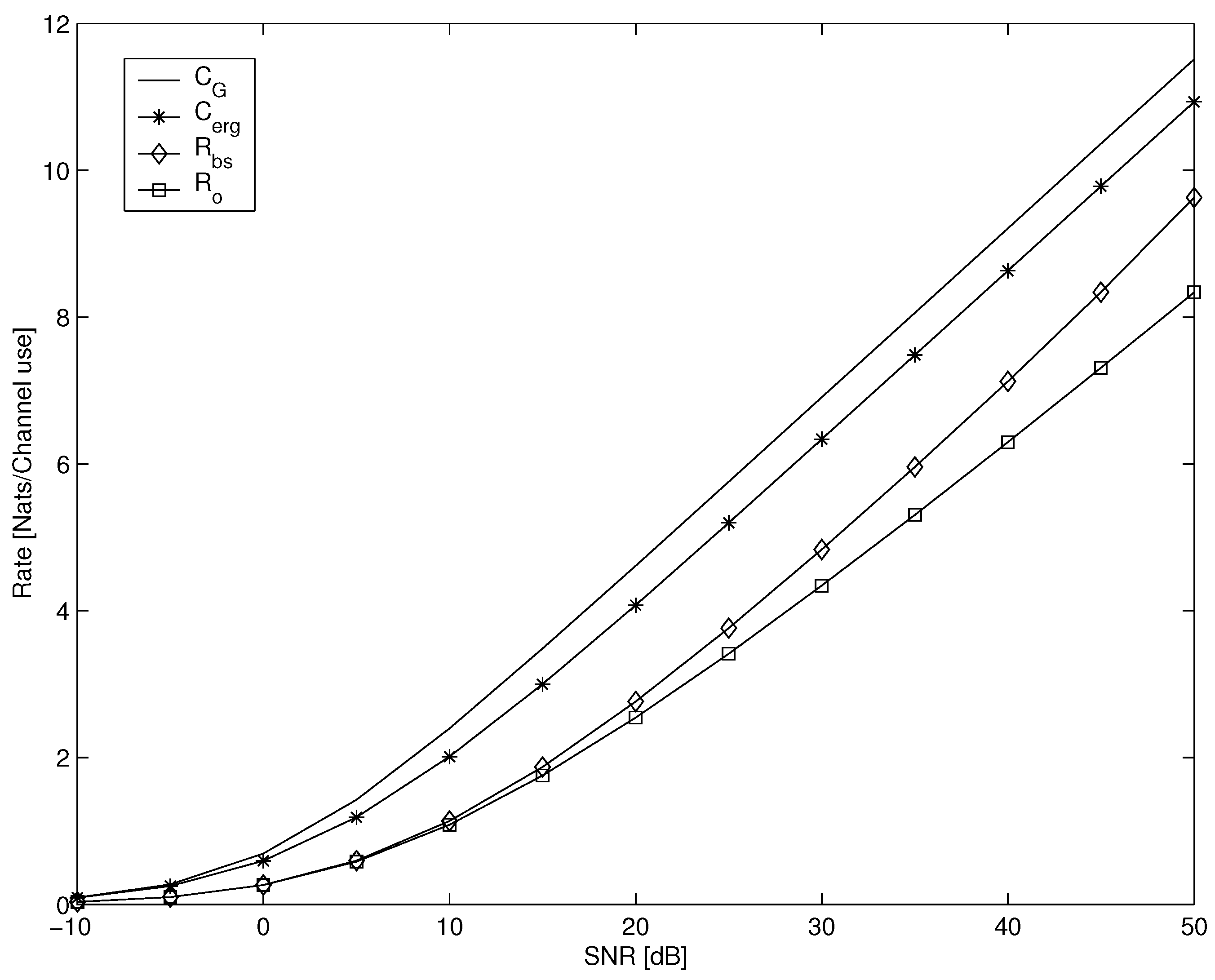
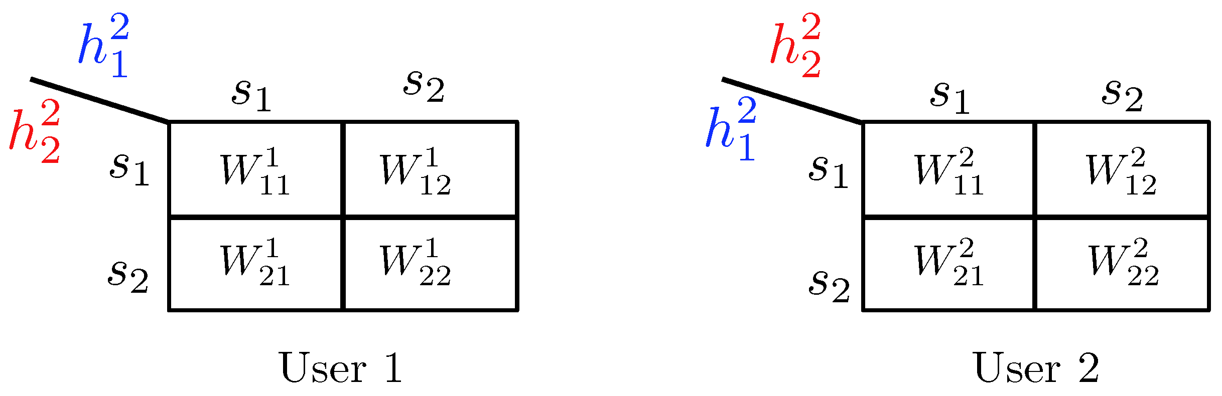
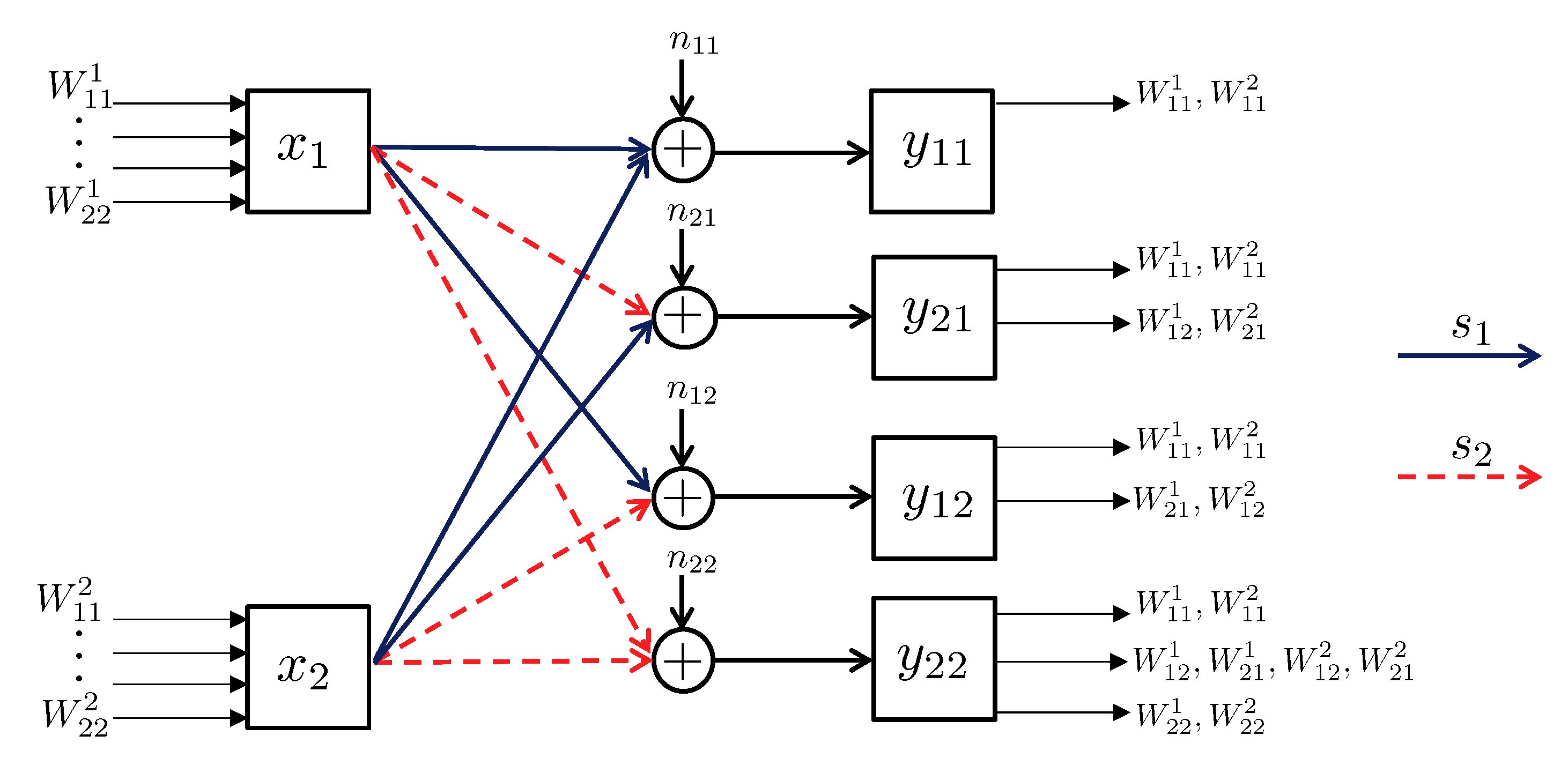
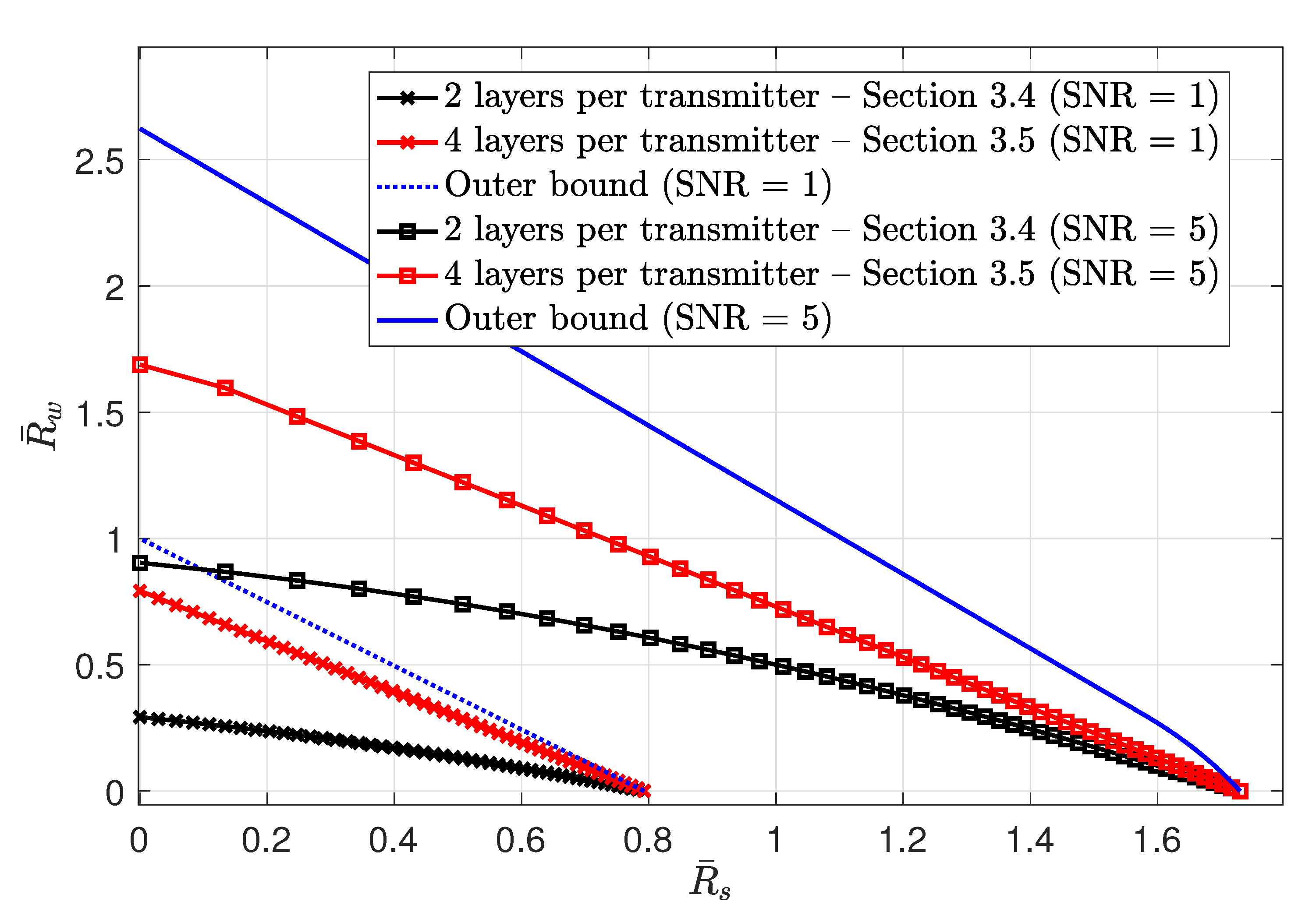
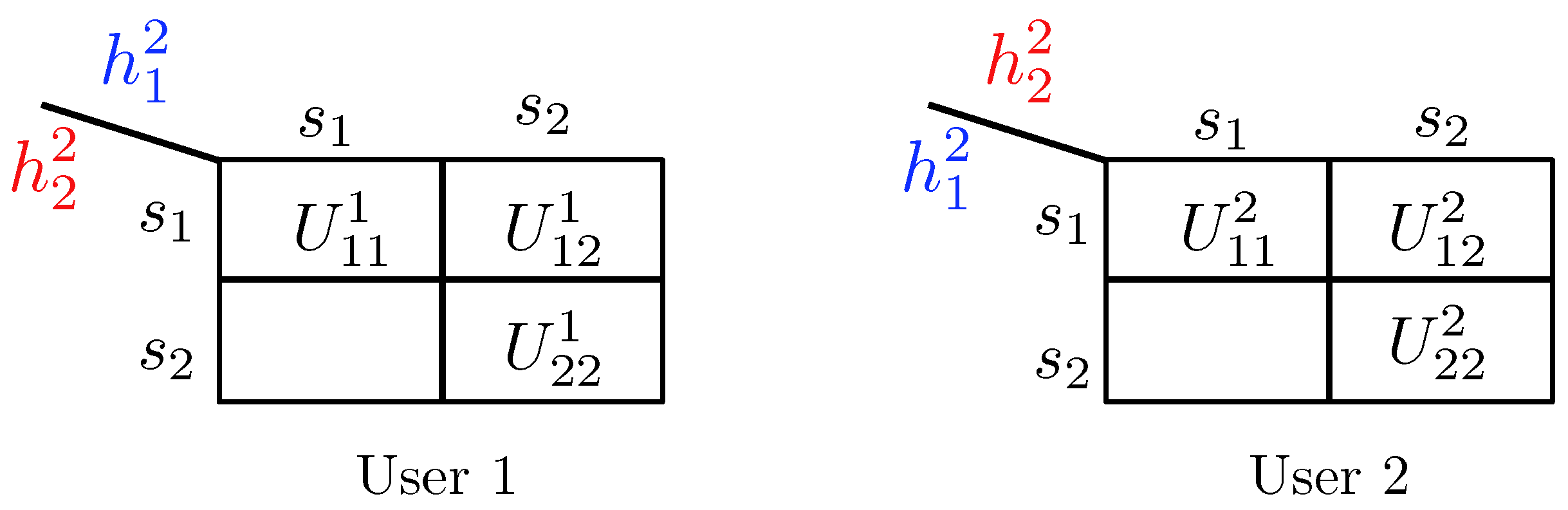
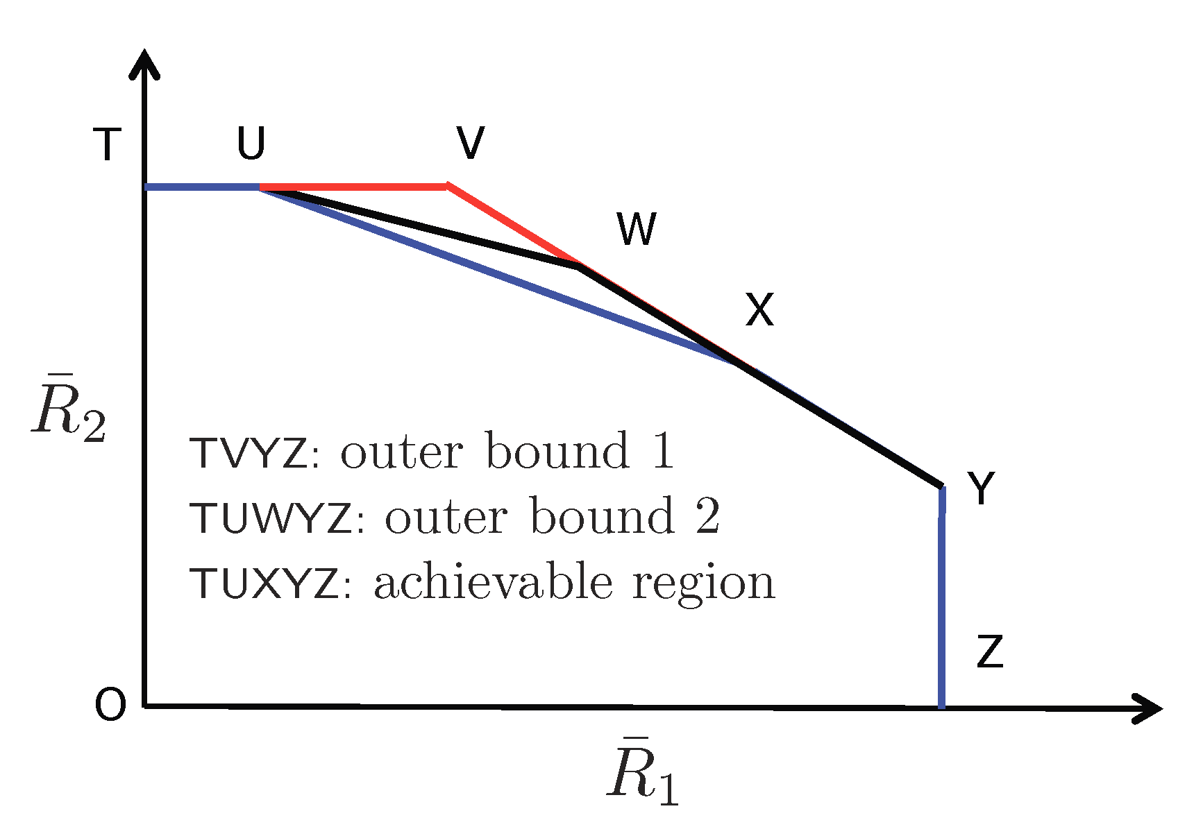
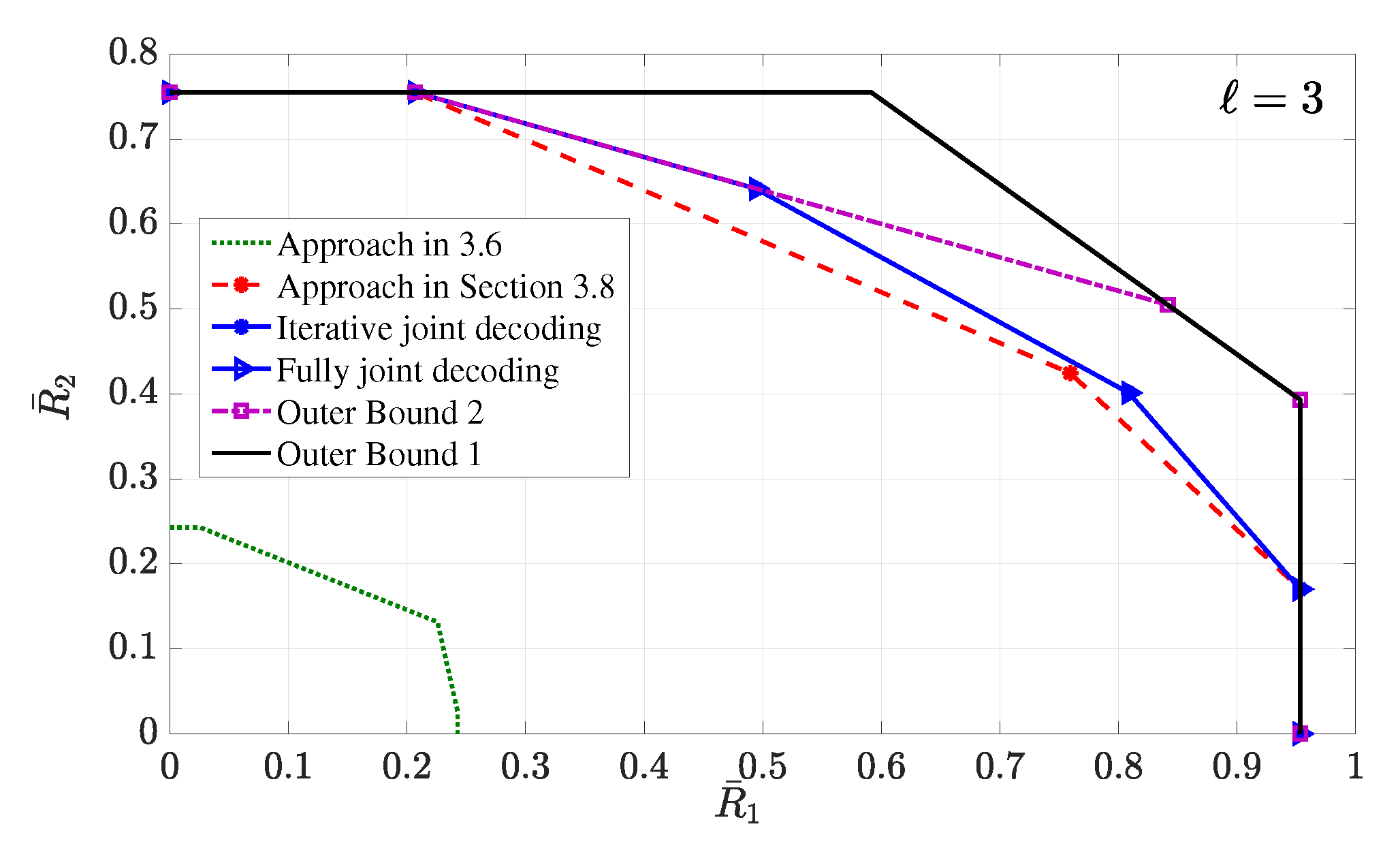
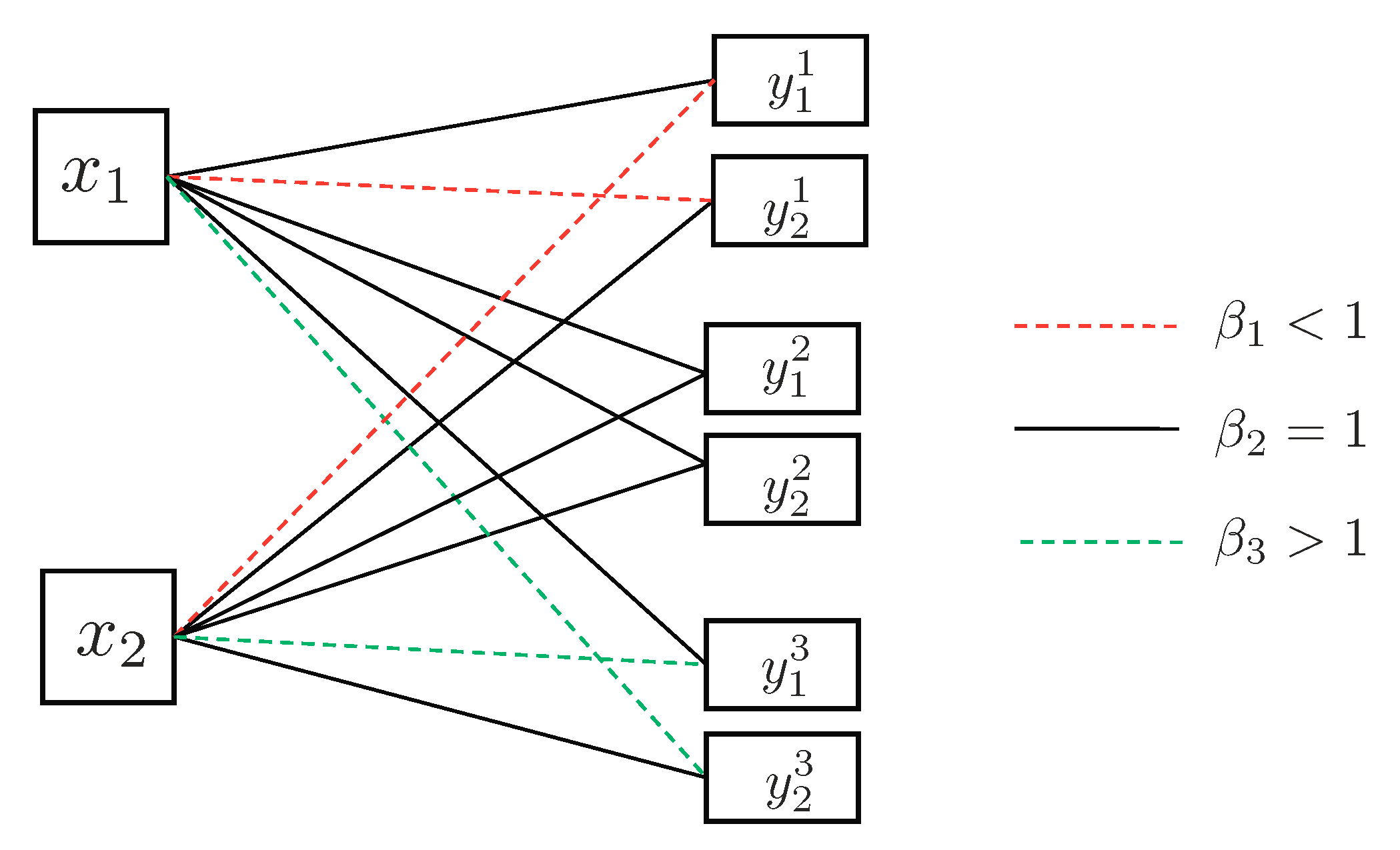
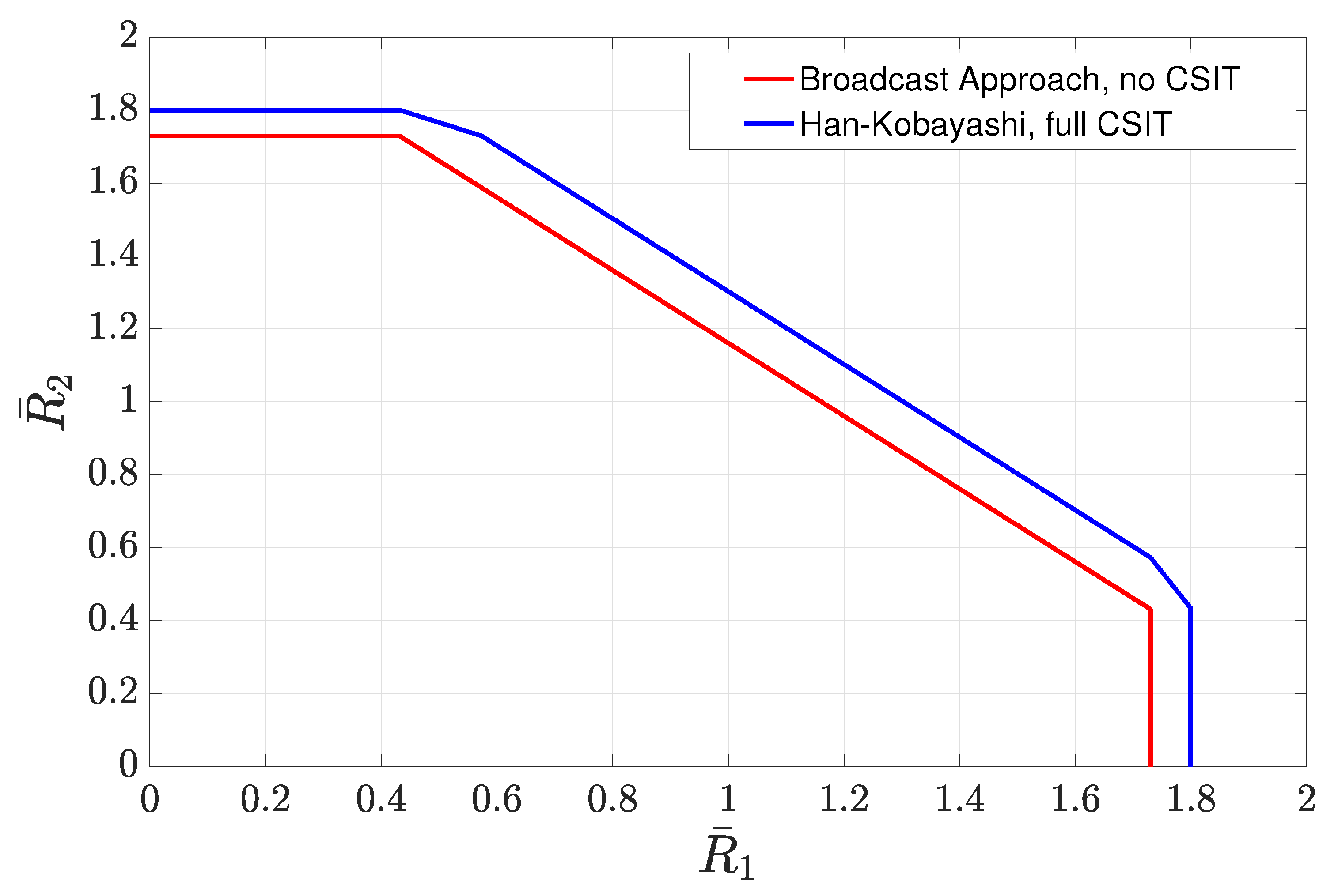
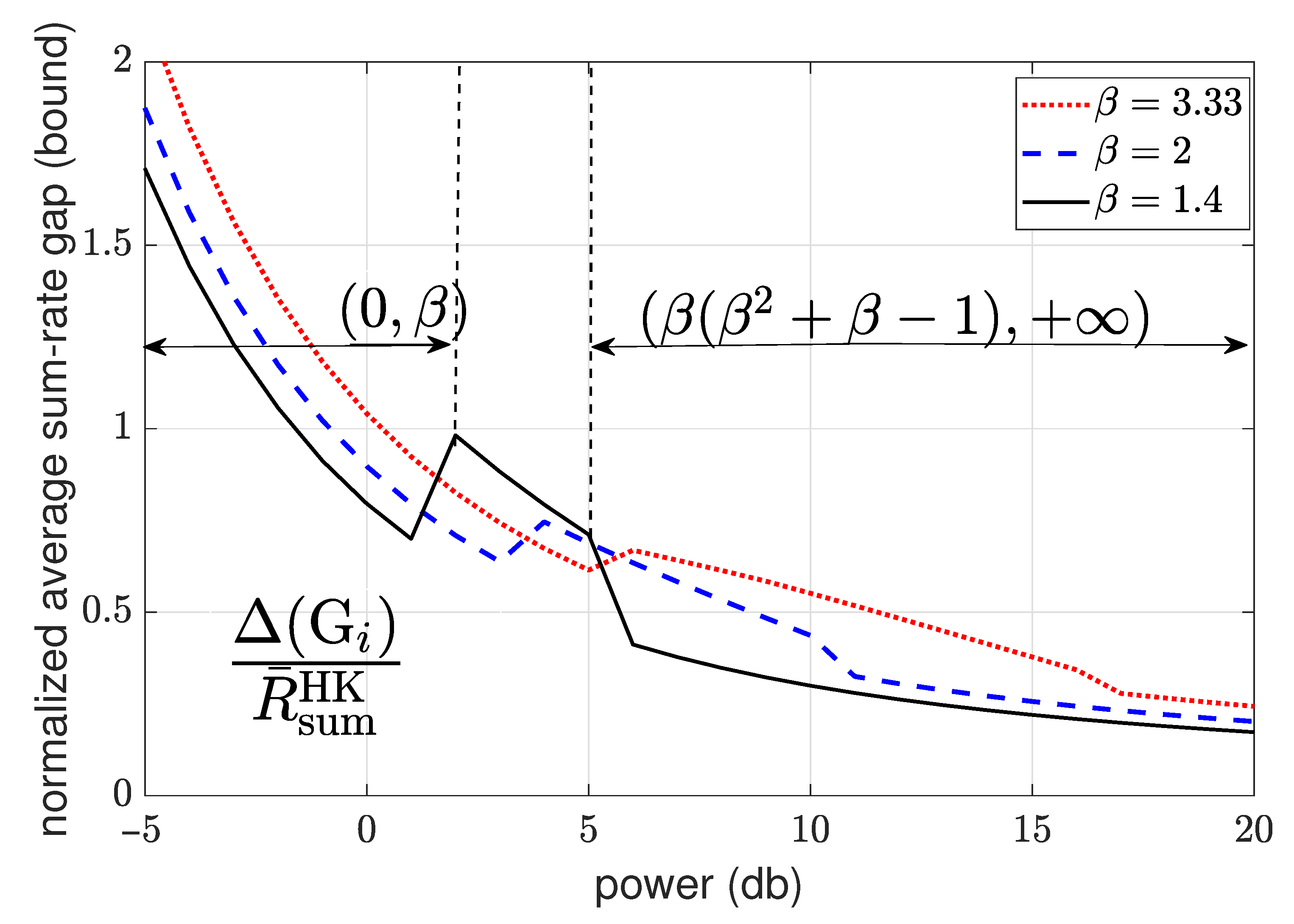
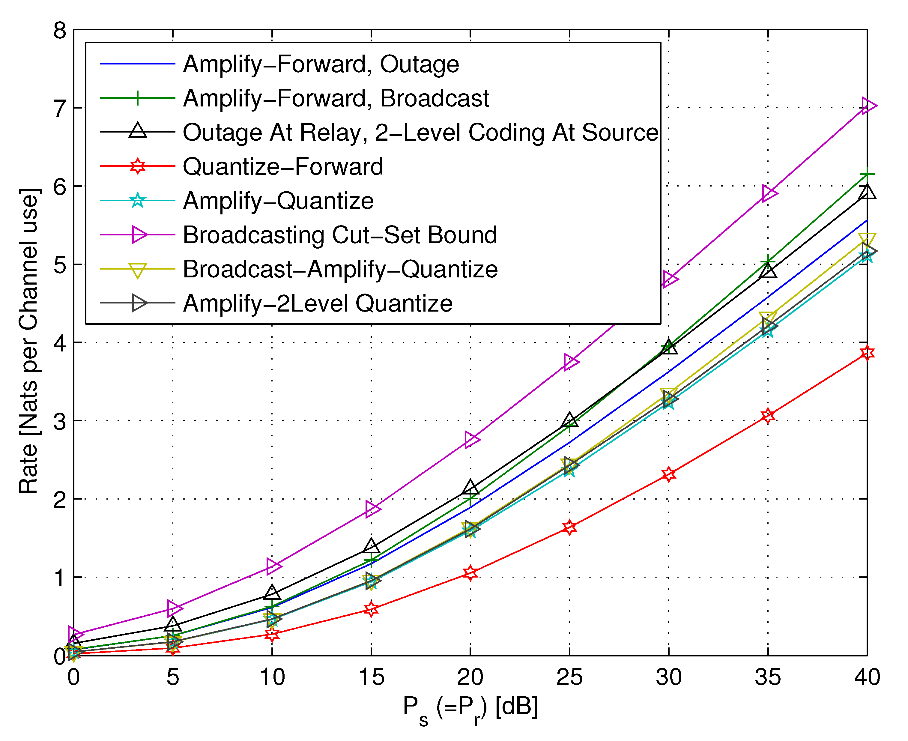
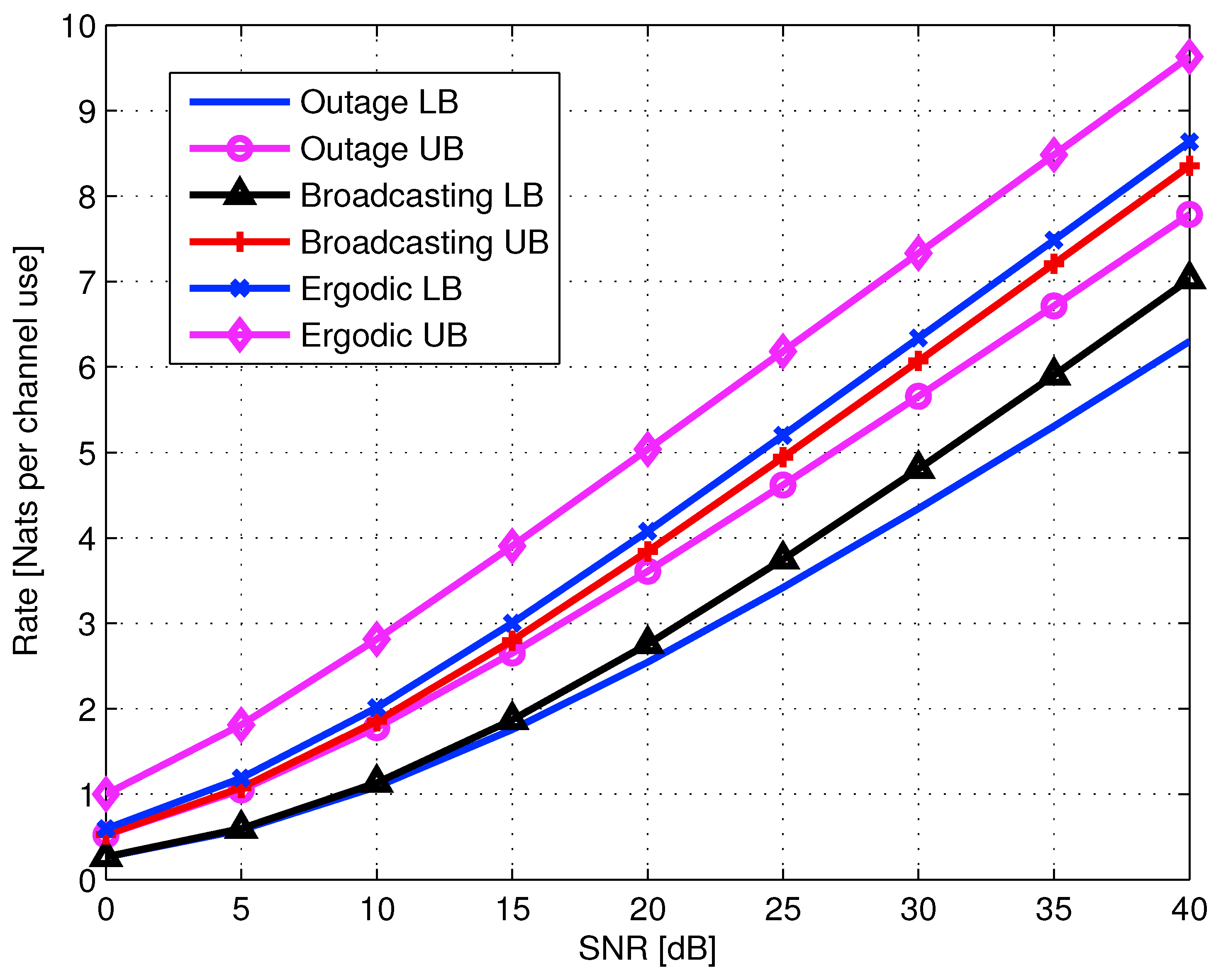
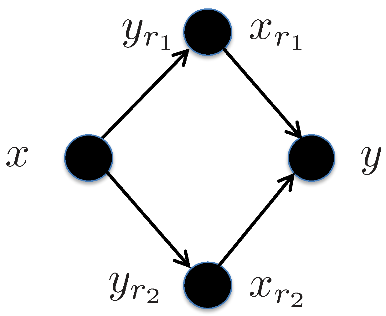
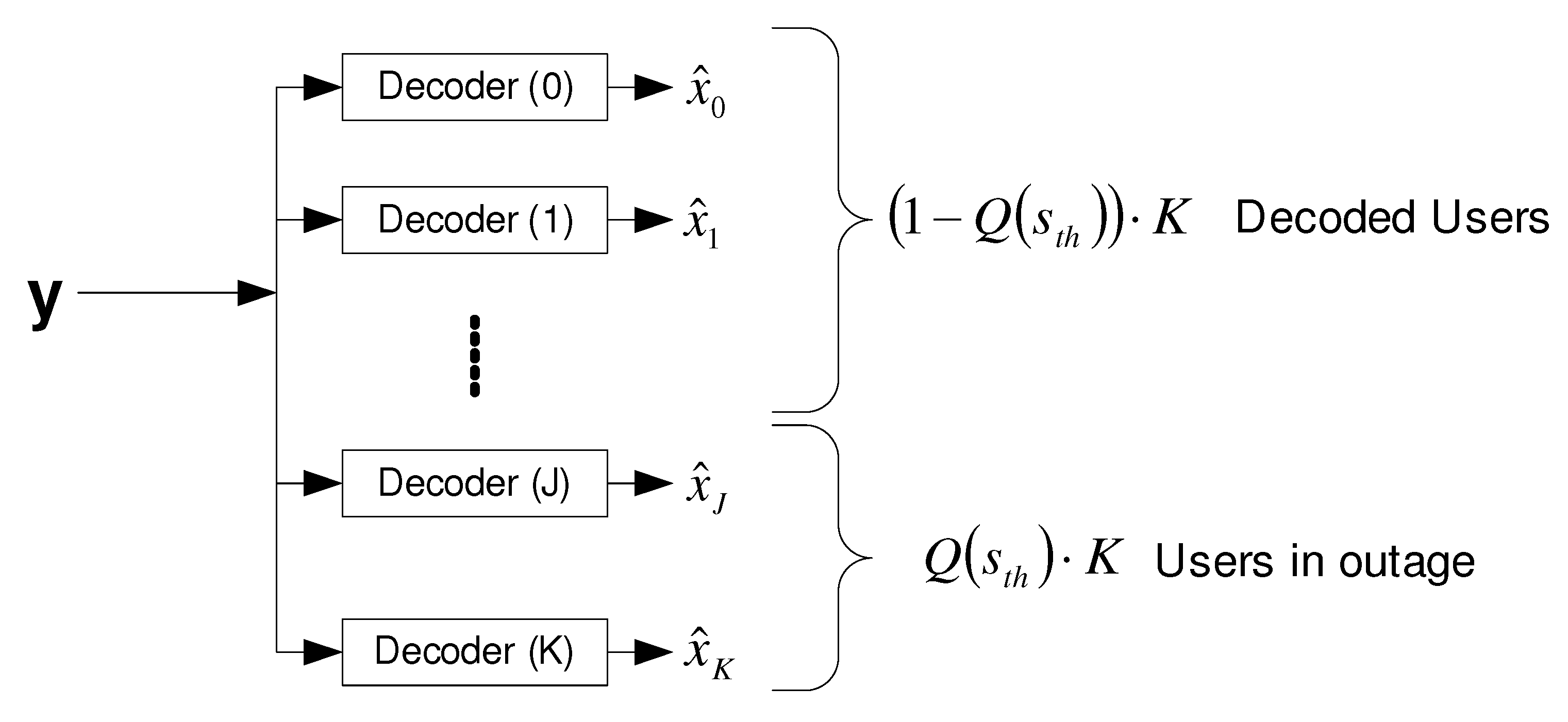
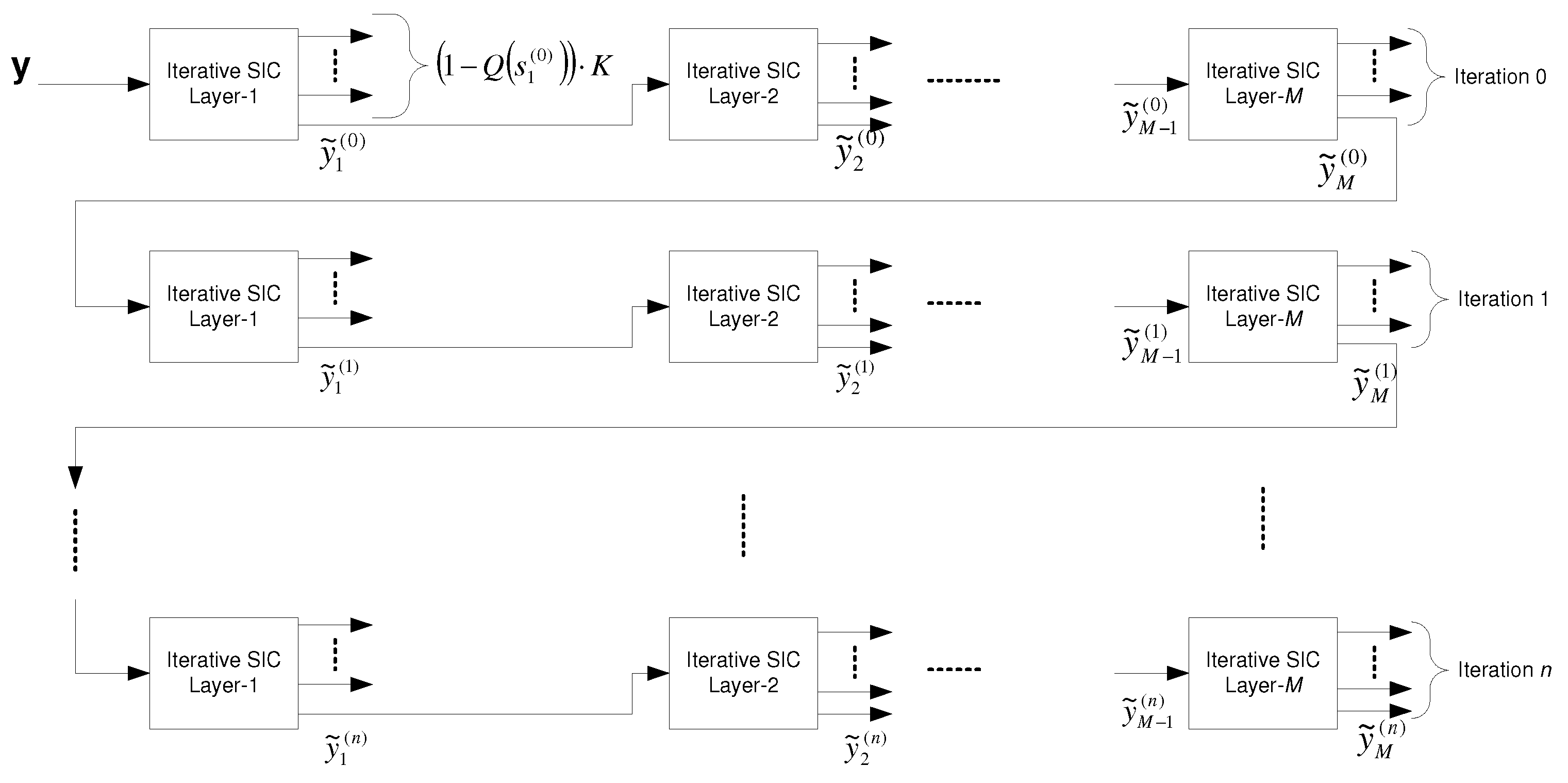
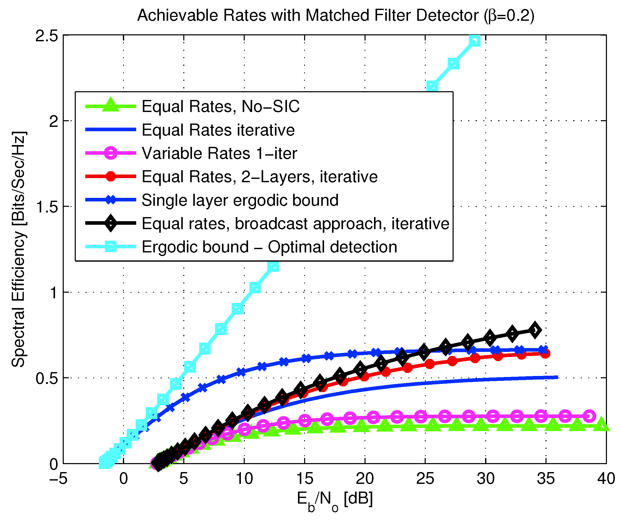
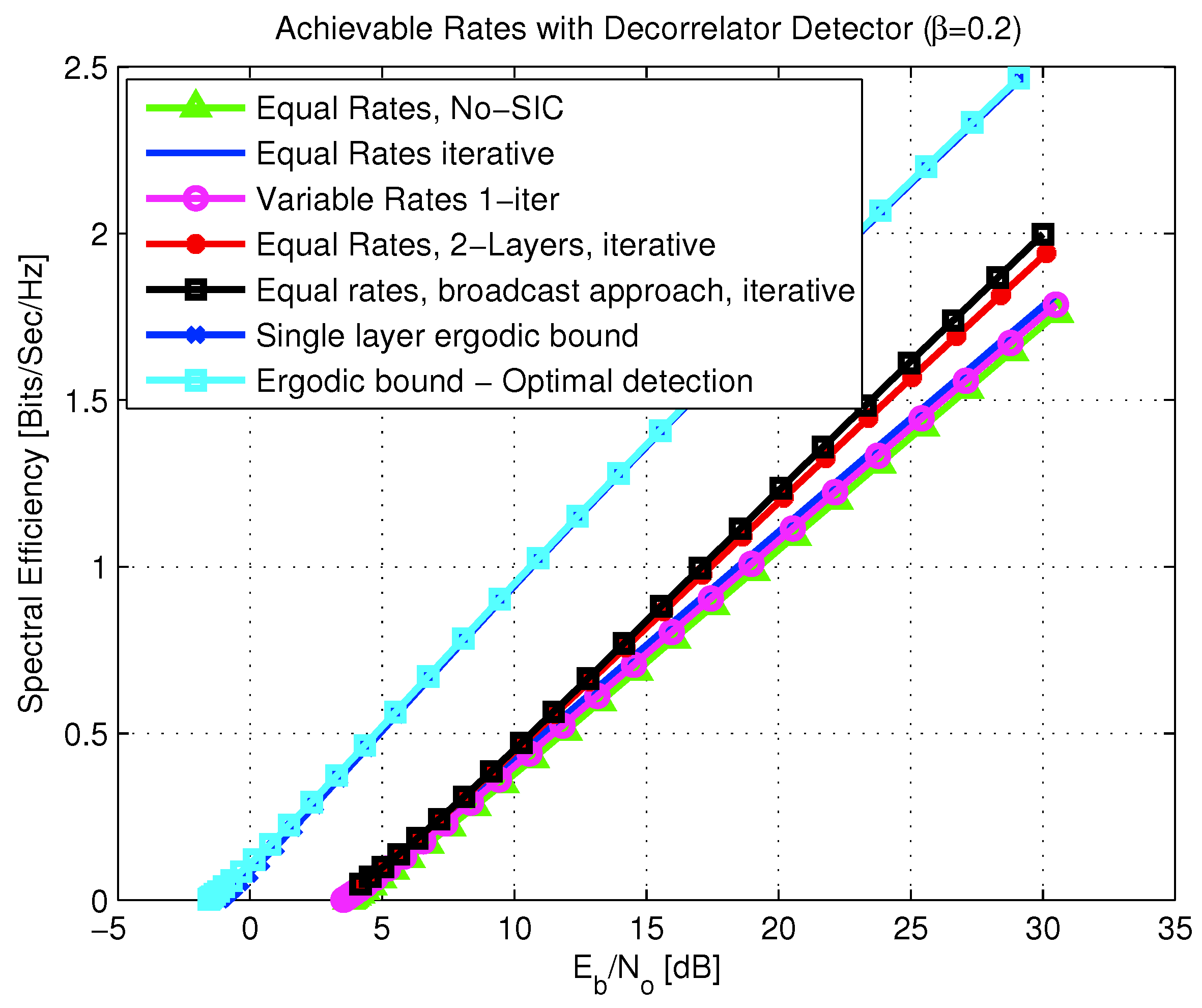
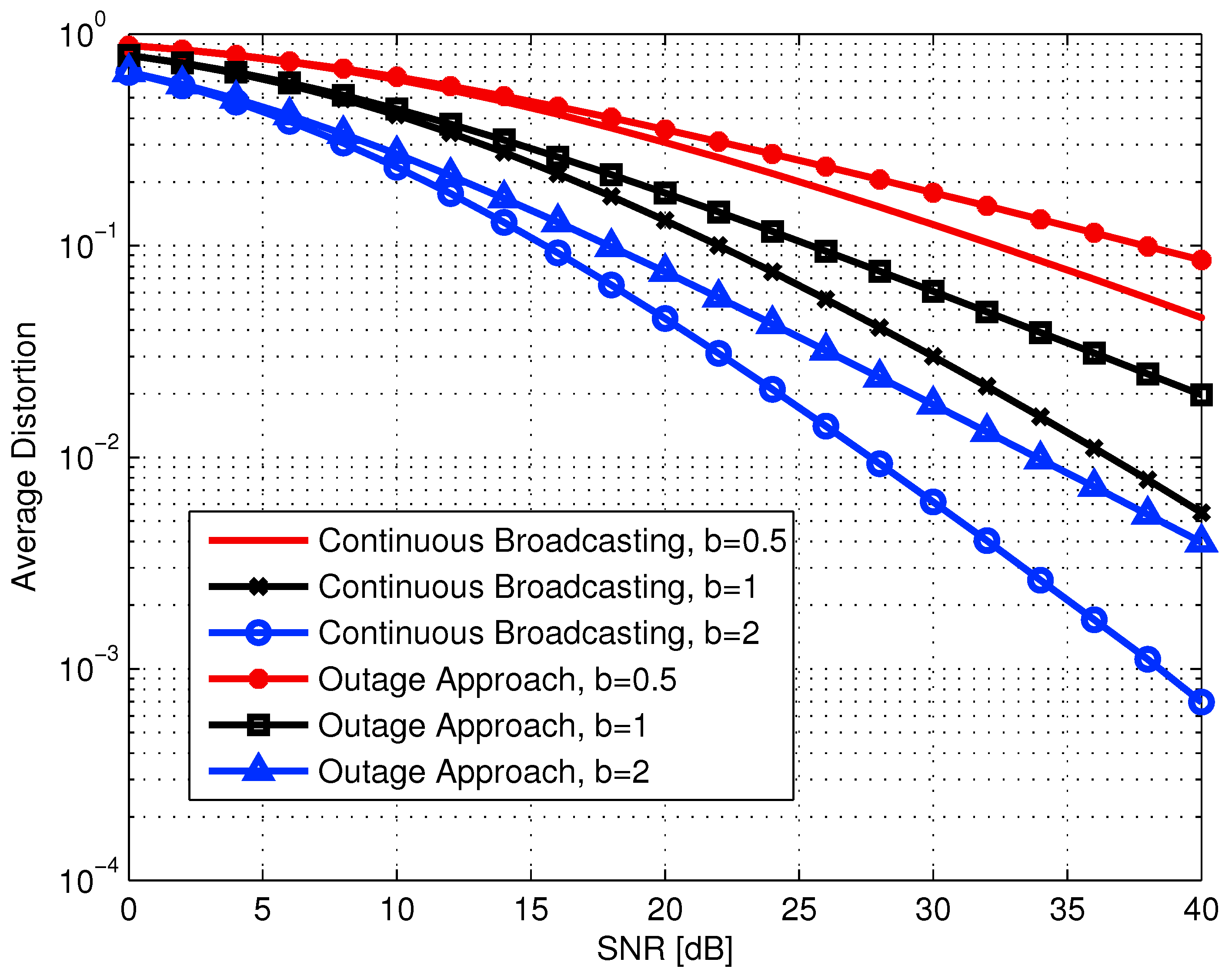
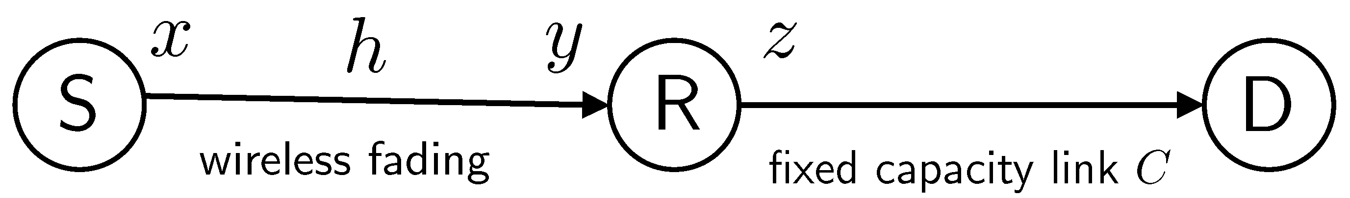
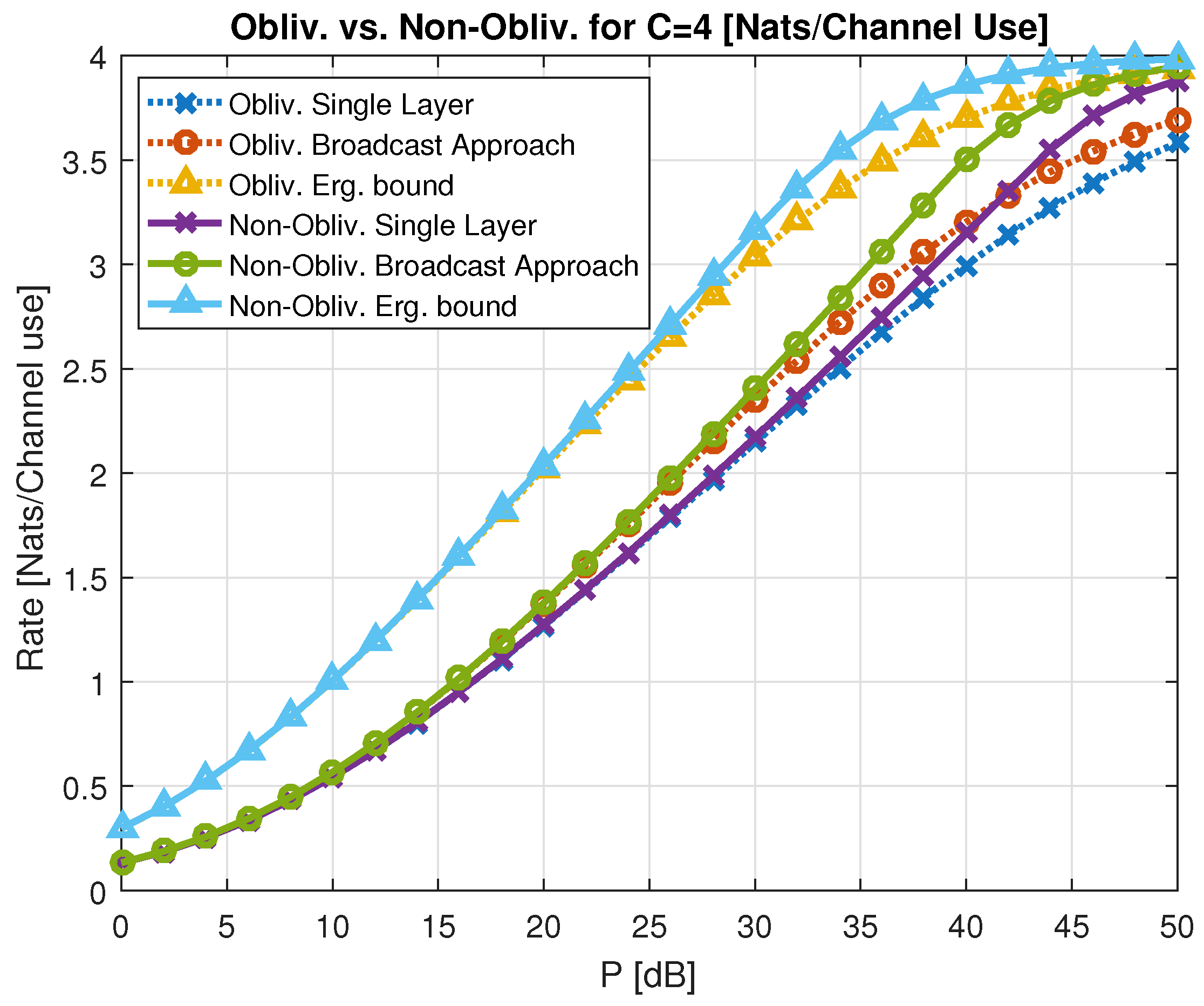
| Decoding Stage 1 | Decoding Stage 2 | |
|---|---|---|
| Stage 1 | Stage 2 | Stage 3 | |
|---|---|---|---|
| ·· | ·· | ||||||
|---|---|---|---|---|---|---|---|
, | , | ·· | · | ·· | , | ||
, | , , , | ·· | · | ·· | , | ||
| · | · | · | ·· | · | ·· | · | |
| · | · | ·· | , | ·· | · | ||
| · | · | · | ·· | · | ·· | · | |
, | , | ·· | · | ·· | , | ||
| Stage 1 | Stage 2 | Stage 3 | Stage 4 | |
|---|---|---|---|---|
| Stage 1 | Stage 2 | |
|---|---|---|
| ⋯ | ⋯ | ||||||
|---|---|---|---|---|---|---|---|
| ⋯ | · | ⋯ | |||||
| ⋯ | · | ⋯ | |||||
| · | · | · | ⋯ | · | ⋯ | · | |
| · | · | ⋯ | ⋯ | · | |||
| · | · | · | ⋯ | · | ⋯ | · | |
| ⋯ | · | ⋯ | |||||
| Receiver | Stage 1 | Stage 2 | Stage 3 | Stage 4 | Stage 5 | Stage 6 | Stage 7 | Stage 8 | Stage 9 |
|---|---|---|---|---|---|---|---|---|---|
| ⋯ | ⋯ | ||||||
|---|---|---|---|---|---|---|---|
| ⋯ | · | ⋯ | |||||
| ⋯ | · | ⋯ | |||||
| · | · | · | ⋯ | · | ⋯ | · | |
| · | · | ⋯ | ⋯ | · | |||
| · | · | · | ⋯ | · | ⋯ | · | |
| ⋯ | · | ⋯ | |||||
Publisher’s Note: MDPI stays neutral with regard to jurisdictional claims in published maps and institutional affiliations. |
© 2021 by the authors. Licensee MDPI, Basel, Switzerland. This article is an open access article distributed under the terms and conditions of the Creative Commons Attribution (CC BY) license (http://creativecommons.org/licenses/by/4.0/).
Share and Cite
Tajer, A.; Steiner, A.; Shamai, S. The Broadcast Approach in Communication Networks. Entropy 2021, 23, 120. https://doi.org/10.3390/e23010120
Tajer A, Steiner A, Shamai S. The Broadcast Approach in Communication Networks. Entropy. 2021; 23(1):120. https://doi.org/10.3390/e23010120
Chicago/Turabian StyleTajer, Ali, Avi Steiner, and Shlomo Shamai (Shitz). 2021. "The Broadcast Approach in Communication Networks" Entropy 23, no. 1: 120. https://doi.org/10.3390/e23010120
APA StyleTajer, A., Steiner, A., & Shamai, S. (2021). The Broadcast Approach in Communication Networks. Entropy, 23(1), 120. https://doi.org/10.3390/e23010120