1. Introduction
The solutions to many information-theoretic problems can be expressed using Shannon’s information measures such as entropy, relative entropy, and mutual information. Other problems require Rényi’s information measures, which generalize Shannon’s. In this paper, we analyze two Rényi measures of dependence,
and
, between random variables
X and
Y taking values in the finite sets
and
, with
being a parameter. (Our notation is similar to the one used for the mutual information: technically,
and
are functions not of
X and
Y, but of their joint probability mass function (PMF)
.) For
, we define
and
as
where
and
denote the set of all PMFs over
and
, respectively;
denotes the Rényi divergence of order
(see (
50) ahead); and
denotes the relative
-entropy (see (
55) ahead). As shown in Proposition 7,
and
are in fact closely related.
The measures
and
have the following operational meanings (see
Section 3):
is related to the optimal error exponents in testing whether the observed independent and identically distributed (IID) samples were generated according to the joint PMF
or an unknown product PMF; and
appears as a penalty term in the sum-rate constraint of distributed task encoding.
The measures
and
share many properties with Shannon’s mutual information [
1], and both are equal to the mutual information when
is one. Except for some special cases, we have no closed-form expressions for
or
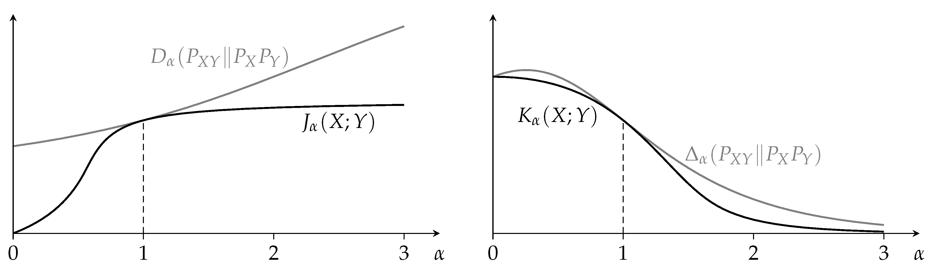
. As illustrated in
Figure 1, unless
is one, the minimum in the definitions of
and
is typically not achieved by
and
. (When
is one, then the minimum is always achieved by
and
; this follows from Proposition 8 and the fact that
.)
The rest of this paper is organized as follows. In
Section 2, we review other generalizations of the mutual information. In
Section 3, we discuss the operational meanings of
and
. In
Section 4, we recall the required Rényi information measures and prove some preparatory results. In
Section 5, we state the properties of
and
. In
Section 6, we prove these properties.
2. Related Work
The measure
was discovered independently from the authors of the present paper by Tomamichel and Hayashi [
2] (Equation (
58)), who, for the case when
, derived some of its properties in [
2] (Appendix A-C).
Other Rényi-based measures of dependence appeared in the past. Notable are those by Sibson [
3], Arimoto [
4], and Csiszár [
5], respectively denoted by
,
, and
:
where, throughout the paper,
denotes the base-2 logarithm;
denotes the Rényi divergence of order
(see (
50) ahead);
denotes the Rényi entropy of order
(see (
45) ahead); and
denotes the Arimoto–Rényi conditional entropy [
4,
6,
7], which is defined for positive
other than one as
(Equation (
4) follows from Proposition 9 ahead, and (6) follows from (
45) and (
8).) An overview of
,
, and
is provided in [
8]. Another Rényi-based measure of dependence can be found in [
9] (Equation (
19)):
The relation between , , and for was established recently:
Proposition 1 ([
10] (Theorem IV.1)).
For every PMF and every , Proof. This is proved in [
10] for a measure-theoretic setting. Here, we specialize the proof to finite alphabets. We first prove (
10):
where (
12) follows from the definition of
in (
1); (
13) follows from Proposition 9 ahead with the roles of
and
swapped; (
15) follows from Jensen’s inequality because
is concave and because
; and (
17) follows from the definition of
in (7).
We next prove (
11):
where (
18) follows from the definition of
in (
1), and (
20) follows from (
4). □
Many of the above Rényi information measures coincide when they are maximized over
with
held fixed: for every conditional PMF
and every positive
other than one,
where
denotes the joint PMF of
X and
Y; (
21) follows from [
4] (Lemma 1); and (
22) follows from [
5] (Proposition 1). It was recently established that, for
, this is also true for
:
Proposition 2 ([
10] (Theorem V.1)).
For every conditional PMF and every , Proof. By Proposition 1, we have for all
By (
22), the left-hand side (LHS) of (
24) is equal to the right-hand side (RHS) of (
25), so (
24) and (
25) both hold with equality. □
Dependence measures can also be based on the
f-divergence
[
11,
12,
13]. Every convex function
satisfying
induces a dependence measure, namely
where (
27) follows from the definition of the
f-divergence. (For
,
is the mutual information.) Such dependence measures are used for example in [
14], and a construction equivalent to (
27) is studied in [
15].
4. Preliminaries
Throughout the paper,
denotes the base-2 logarithm,
and
are finite sets,
denotes a joint PMF over
,
denotes a PMF over
, and
denotes a PMF over
. We use
P and
Q as generic PMFs over a finite set
. We denote by
the support of
P, and by
the set of all PMFs over
. When clear from the context, we often omit sets and subscripts: for example, we write
for
,
for
,
for
, and
for
. Whenever a conditional probability
is undefined because
, we define
. We denote by
the indicator function that is one if the condition is satisfied and zero otherwise. In the definitions below, we use the following conventions:
The Rényi entropy of order
[
21] is defined for positive
other than one as
For
being zero, one, or infinity, we define by continuous extension of (
45)
where
is the Shannon entropy. With this extension to
, the Rényi entropy satisfies the following basic properties:
Proposition 3 ([
5]).
Let P be a PMF. Then,- (i)
For all , . If , then if and only if X is distributed uniformly over .
- (ii)
The mapping is nonincreasing on .
- (iii)
The mapping is continuous on .
The relative entropy (or Kullback–Leibler divergence) is defined as
The Rényi divergence of order
[
21,
22] is defined for positive
other than one as
where we read
as
if
. For
being zero, one, or infinity, we define by continuous extension of (
50)
With this extension to , the Rényi divergence satisfies the following basic properties:
Proposition 4. Let P and Q be PMFs. Then,
- (i)
For all , is finite if and only if . For all , is finite if and only if .
- (ii)
For all , . If , then if and only if .
- (iii)
For every , the mapping is continuous.
- (iv)
The mapping is nondecreasing on .
- (v)
The mapping is continuous on .
Proof. Part (i) follows from the definition of
and the conventions (
44), and Parts (ii)–(v) are shown in [
22]. □
The Rényi divergence for negative
is defined as
(We use negative
only in Lemma 19. More about negative orders can be found in [
22] (Section V). For other applications of negative orders, see [
23] (Proof of Theorem 1 and Example 1).)
The relative
-entropy [
24,
25] is defined for positive
other than one as
where we read
as
if
. The relative
-entropy appears in mismatched guessing [
26], mismatched source coding [
26] (Theorem 8), and mismatched task encoding [
19] (Section IV). It also arises in robust parameter estimation and constrained compression settings [
25] (Section II). For
being zero, one, or infinity, we define by continuous extension of (
55)
where
and
is the cardinality of this set. With this extension to
, the relative
-entropy satisfies the following basic properties:
Proposition 5. Let P and Q be PMFs. Then,
- (i)
For all , is finite if and only if . For all , is finite if and only if .
- (ii)
For all , . If , then if and only if .
- (iii)
For every , the mapping is continuous.
- (iv)
The mapping is continuous on .
(Part (i) differs from [
19] (Proposition IV.1), where the conventions for
differ from ours. Our conventions are compatible with [
24,
25], and, as stated in Part (iii), they result in the continuity of the mapping
.)
Proof of Proposition 5. Part (i) follows from the definition of
in (
55) and the conventions (
44). For
, Part (ii) follows from [
19] (Proposition IV.1); for
, Part (ii) holds because
; and for
, Part (ii) follows from the definition of
. Part (iii) follows from the definition of
, and Part (iv) follows from [
19] (Proposition IV.1). □
In the rest of this section, we prove some auxiliary results that we need later (Propositions 6–9). We first establish the relation between and .
Proposition 6 ([
26] (Section V, Property 4)).
Let P and Q be PMFs, and let . Then,where the PMFs and are given by Proof. If
, then (
59) holds because
,
, and
. Now let
. Because
and
are zero if and only if
and
are zero, respectively, the LHS of (
59) is finite if and only if its RHS is finite. If
is finite, then (
59) follows from a simple computation. □
In light of Proposition 6, and are related as follows:
Proposition 7. Let be a joint PMF, and let . Then,where the joint PMF of and is given by Proof. Let
. For fixed PMFs
and
, define the transformed PMFs
,
, and
as
Then,
where (
67) holds by the definition of
; (
68) follows from Proposition 6; (
69) holds because
; (
70) holds because the transformations (
65) and (66) are bijective on the set of PMFs over
and
, respectively; and (
71) holds by the definition of
. □
The next proposition provides a characterization of the mutual information that parallels the definitions of and . Because , this also shows that and reduce to the mutual information when is one.
Proposition 8 ([
27] (Theorem 3.4)).
Let be a joint PMF. Then, for all PMFs and ,with equality if and only if and . Thus, Proof. A simple computation reveals that
which implies (
72) because
with equality if and only if
. Thus, (
73) holds because
. □
The last proposition of this section is about a precursor to
, namely, the minimization of
with respect to
only, which can be carried out explicitly. (This proposition extends [
5] (Equation (
13)) and [
2] (Lemma 29).)
Proposition 9. Let be a joint PMF and a PMF. Then, for every ,with the conventions of (44). If the RHS of (75) is finite, then the minimum is achieved uniquely by For ,with the conventions of (44). If the RHS of (77) is finite, then the minimum is achieved uniquely by Proof. We first treat the case
. If the RHS of (
75) is infinite, then the conventions imply that
is infinite for every
, so (
75) holds. Otherwise, if the RHS of (
75) is finite, then the PMF
given by (
76) is well-defined, and a simple computation shows that for every
,
The only term on the RHS of (
79) that depends on
is
. Because
with equality if and only if
(Proposition 4), (
79) implies (
75) and (
76).
The case
is analogous: if the RHS of (
77) is infinite, then the LHS of (
77) is infinite, too; and if the RHS of (
77) is finite, then the PMF
given by (
78) is well-defined, and a simple computation shows that for every
,
The only term on the RHS of (
80) that depends on
is
. Because
with equality if and only if
(Proposition 4), (
80) implies (
77) and (
78). □
5. Two Measures of Dependence
We state the properties of
in Theorem 1 and those of
in Theorem 2. The enumeration labels in the theorems refer to the lemmas in
Section 6 where the properties are proved. (The enumeration labels are not consecutive because, in order to avoid forward references in the proofs, the order of the results in
Section 6 is not the same as here.)
Theorem 1. Let X, , , Y, , , and Z be random variables taking values in finite sets. Then:
- (Lemma 1)
For every , the minimum in the definition of exists and is finite.
The following properties of the mutual information [28] (Chapter 2) are also satisfied by : - (Lemma 2)
For all , . If , then if and only if X and Y are independent (nonnegativity).
- (Lemma 3)
For all , (symmetry).
- (Lemma 4)
If form a Markov chain, then for all (data-processing inequality).
- (Lemma 12)
If the pairs and are independent, then for all (additivity).
- (Lemma 13)
For all , with equality if and only if , X is distributed uniformly over , and .
- (Lemma 14)
For every , is concave in for fixed .
Moreover:
- (Lemma 5)
.
- (Lemma 6)
Let and be bijective functions, and let be the matrix whose Row-i Column-j entry equals . Then,where denotes the largest singular value of . (Because the singular values of a matrix are invariant under row and column permutations, the result does not depend on f or g.) - (Lemma 7)
.
- (Lemma 8)
Thus, being the minimum of concave functions in α, the mapping is concave on .
- (Lemma 9)
The mapping is nondecreasing on .
- (Lemma 10)
The mapping is continuous on .
- (Lemma 11)
If with probability one, then
The minimization problem in the definition of has the following characteristics:
- (Lemma 15)
For every , the mapping is convex, i.e., for all with , all , and all , For , the mapping need not be convex.
- (Lemma 16)
Let . If achieves the minimum in the definition of , then there exist positive normalization constants c and d such thatwith the conventions of (44). The case is similar: if achieves the minimum in the definition of , then there exist positive normalization constants c and d such thatwith the conventions of (44). (If , then and by Proposition 8.) Thus, for all , both inclusions and hold. - (Lemma 20)
For every , the mapping has a unique minimizer. This need not be the case when .
The measure can also be expressed as follows:
- (Lemma 17)
For all ,where is defined asand is given explicitly as follows: for ,with the conventions of (44); and for ,with the conventions of (44). For every , the mapping is convex. For , the mapping need not be convex. - (Lemma 18)
For all ,where For every , the mapping is concave. For all and all , the statement is equivalent to .
- (Lemma 19)
For all ,where the minimization is over all PMFs satisfying ; for negative α is given by (54); and Gallager’s function [29] is defined as
We now move on to the properties of . Some of these properties are derived from their counterparts of using the relation described in Proposition 7.
Theorem 2. Let X, , , Y, , , and Z be random variables taking values in finite sets. Then:
- (Lemma 21)
For every , the minimum in the definition of in (2) exists and is finite.
The following properties of the mutual information are also satisfied by :
- (Lemma 22)
For all , . If , then if and only if X and Y are independent (nonnegativity).
- (Lemma 23)
For all , (symmetry).
- (Lemma 34)
If the pairs and are independent, then for all (additivity).
- (Lemma 35)
For all , .
Unlike the mutual information, does not satisfy the data-processing inequality:
- (Lemma 36)
There exists a Markov chain for which .
Moreover:
- (Lemma 24)
For all ,where is the following weighted power mean [30] (Chapter III): For ,where for , we read as and use the conventions (44); and for , using the convention , - (Lemma 25)
For ,where in the RHS of (102), we use the conventions (44). The inequality can be strict, so need not be continuous at . - (Lemma 26)
.
- (Lemma 27)
Let and be bijective functions, and let be the matrix whose Row-i Column-j entry equals . Then,where denotes the largest singular value of . (Because the singular values of a matrix are invariant under row and column permutations, the result does not depend on f or g.) - (Lemma 28)
.
- (Lemma 29)
The mapping need not be monotonic on .
- (Lemma 30)
The mapping is nonincreasing on .
- (Lemma 31)
The mapping is continuous on . (See Lemma 25 for the behavior at .)
- (Lemma 32)
If with probability one, then - (Lemma 33)
For every , the mapping in the definition of in (2) has a unique minimizer. This need not be the case when .
6. Proofs
In this section, we prove the properties of
and
stated in
Section 5.
Lemma 1. For every , the minimum in the definition of exists and is finite.
Proof. Let . Then is finite because is finite and because the Rényi divergence is nonnegative. The minimum exists because the set is compact and the mapping is continuous. □
Lemma 2. For all , . If , then if and only if X and Y are independent (nonnegativity).
Proof. The nonnegativity follows from the definition of because the Rényi divergence is nonnegative for . If X and Y are independent, then , and the choice and in the definition of achieves . Conversely, if , then there exist PMFs and satisfying . If, in addition, , then by Proposition 4, and hence X and Y are independent. □
Lemma 3. For all , (symmetry).
Proof. The definition of is symmetric in X and Y. □
Lemma 4. If form a Markov chain, then for all (data-processing inequality).
Proof. Let
form a Markov chain, and let
. Let
and
be PMFs that achieve the minimum in the definition of
, so
Define the PMF
as
(As noted in the preliminaries, we define
when
.) We show below that
which implies the data-processing inequality because
where (
109) holds by the definition of
; (
110) follows from (
108); and (
111) follows from (
106).
The proof of (
108) is based on the data-processing inequality for the Rényi divergence. Define the conditional PMF
as
If
, then the marginal distribution of
and
is
where (
114) follows from (
112); and (
115) holds because
X,
Y, and
Z form a Markov chain. If
, then the marginal distribution of
and
is
where (
118) follows from (
112), and (
119) follows from (
107). Finally, we are ready to prove (
108):
where (
120) follows from (
116) and (
119), and where (
121) follows from the data-processing inequality for the Rényi divergence [
22] (Theorem 9). □
Lemma 5. .
Proof. By Lemma 2, , so it suffices to show that . Let satisfy . Define the PMF as and the PMF as . Then, , so by the definition of . □
Lemma 6. Let and be bijective functions, and let be the matrix whose Row-i Column-j entry equals . Then,where denotes the largest singular value of . (Because the singular values of a matrix are invariant under row and column permutations, the result does not depend on f or g.) Proof. By the definitions of
and the Rényi divergence,
The claim follows from (
123) because
where
and
are column vectors with
and
elements, respectively; (
124) is shown below; (125) follows from the Cauchy–Schwarz inequality
, which holds with equality if
and
are linearly dependent; and (126) holds because the spectral norm of a matrix is equal to its largest singular value [
31] (Example 5.6.6).
We now prove (
124). Let
and
be vectors that satisfy
, and define the PMFs
and
as
and
, where
and
denote the inverse functions of
f and
g, respectively. Then,
where (
128) holds because all the entries of
are nonnegative, and in (
129), we changed the summation variables to
and
. It remains to show that equality can be achieved in (
128) and (
130). To that end, let
and
be PMFs that achieve the maximum on the RHS of (
130), and define the vectors
and
as
and
. Then,
, and (
128) and (
130) hold with equality, which proves (
124). □
Lemma 7. .
Proof. This follows from Proposition 8 because in the definition of is equal to . □
Lemma 8. For all ,Thus, being the minimum of concave functions in α, the mapping is concave on . Proof. For
, (
131) holds because
with equality if
. For
,
where (
132) holds by the definition of
; (
133) follows from [
22] (Theorem 30); and (
134) follows from Proposition 8 after swapping the minima.
For
, define the sets
Then,
where (
137) follows from the definition of
because
and because the mapping
is continuous; (
138) follows from [
22] (Theorem 30); (
139) follows from a minimax theorem and is justified below; and (
140) follows from Proposition 8, a continuity argument, and the observation that
is infinite if
.
We now verify the conditions of Ky Fan’s minimax theorem [
32] (Theorem 2), which will establish (
139). (We use Ky Fan’s minimax theorem because it does not require that the set
be compact, and having a noncompact set
helps to guarantee that the function
f defined next takes on finite values only. A brief proof of Ky Fan’s minimax theorem appears in [
33].) Let the function
be defined by the expression in square brackets in (
139), i.e.,
We check that
- (i)
the sets and are convex;
- (ii)
the set is compact;
- (iii)
the function f is real-valued;
- (iv)
for every , the function f is continuous in ;
- (v)
for every , the function f is convex in ; and
- (vi)
for every , the function f is concave in the pair .
Indeed, Parts (i) and (ii) are easy to see; Part (iii) holds because both relative entropies on the RHS of (
141) are finite by our definitions of
and
; and to show Parts (iv)–(vi), we rewrite
f as:
From (
142), we see that Part (iv) holds by our definitions of
and
; Part (v) holds because the entropy is a concave function (so
is convex), because linear functionals of
are convex, and because the sum of convex functions is convex; and Part (vi) holds because the logarithm is a concave function and because a nonnegative weighted sum of concave functions is concave. (In Ky Fan’s theorem, weaker conditions than Parts (i)–(vi) are required, but it is not difficult to see that Parts (i)–(vi) are sufficient.)
The last claim, namely, that the mapping
is concave on
, is true because the expression in square brackets on the RHS of (
131) is concave in
for every
and because the pointwise minimum preserves the concavity. □
Lemma 9. The mapping is nondecreasing on .
Proof. This is true because for every
with
,
which holds because the Rényi divergence is nondecreasing in
(Proposition 4). □
Lemma 10. The mapping is continuous on .
Proof. By Lemma 8, the mapping is concave on , thus it is continuous on , which implies that is continuous on .
We next prove the continuity at
. Let
and
be PMFs that achieve the minimum in the definition of
. Then, for all
,
where (
145) holds because
is nondecreasing (Lemma 9), and (
146) holds by the definition of
. The Rényi divergence is continuous in
(Proposition 4), so (
144)–(
146) and the sandwich theorem imply that
is continuous at
.
We continue with the continuity at
. Define
Then, for all
,
where (
148) holds because
is nondecreasing (Lemma 9), and (
149) and (
152) hold by the definitions of
and the Rényi divergence. The RHS of (
152) tends to
as
tends to infinity, so
is continuous at
by the sandwich theorem.
It remains to show the continuity at
. Let
, and let
. Then, for all PMFs
and
,
where (
153) holds because
and because the Rényi divergence is nondecreasing in
(Proposition 4); (
156) follows from the Cauchy–Schwarz inequality; and (
157) holds because
where (
159) follows from the Cauchy–Schwarz inequality, and (
161) holds because
and because the Rényi divergence is nonnegative for positive orders (Proposition 4). Thus, for all
,
where (
162) follows from (
158) if
and from Proposition 8 if
; and (
164) holds by the definition of
. The Rényi divergence is continuous in
(Proposition 4), thus (
162)–(
164) and the sandwich theorem imply that
is continuous at
. □
Lemma 11. If with probability one, then Proof. We show below that (
165) holds for
. Thus, (
165) holds also for
because both its sides are continuous in
: its LHS by Lemma 10, and its RHS by the continuity of the Rényi entropy (Proposition 3).
Fix
. Then,
where (
166) follows from Proposition 9, and (
168) holds because
First consider the case
. Define
. Then, for all
,
where (
171) holds because
is a PMF. Because
, Proposition 4 implies that
with equality if
. This together with (
168) and (
172) establishes (
165).
Now consider the case
. For all
,
where (
173) holds because
for all
and because
. The inequalities (
173) and (
174) both hold with equality when
, where
is such that
. Thus,
Now (
165) follows:
where (
177) follows from (
168); (178) holds because
; (
179) follows from (
176); and (
180) follows from the definition of
. □
Lemma 12. If the pairs and are independent, then for all (additivity).
Proof. Let the pairs
and
be independent. For
, we establish the lemma by showing the following two inequalities:
Because
is continuous in
(Lemma 10), this will also establish the lemma for
.
To show (
181), let
and
be PMFs that achieve the minimum in the definition of
, and let
and
be PMFs that achieve the minimum in the definition of
, so
Then, (
181) holds because
where (
185) holds by the definition of
as a minimum; (186) follows from a simple computation using the independence hypothesis
; and (
187) follows from (
183) and (184).
To establish (182), we consider the cases
and
separately, starting with
. Let
and
be PMFs that achieve the minimum in the definition of
, so
Define the function
as
and let
be such that
Define the PMFs
and
as
Then,
where (
193) follows from (
188); (194) holds by the independence hypothesis
; (
195) follows from (
189); (
196) follows from (
190); and (
197) follows from (
191) and (192). Taking the logarithm and multiplying by
establishes (182):
where (
199) holds by the definition of
and
.
The proof of (182) for
is essentially the same as for
: Replace the minimum in (
190) by a maximum. Inequality (
196) is then reversed, but (
198) continues to hold because
. Inequality (
199) also continues to hold, and (
198) and (
199) together imply (182).
Lemma 13. For all , with equality if and only if , X is distributed uniformly over , and .
Proof. Throughout the proof, define
. We first show that
for all
:
where (
200) follows from the data-processing inequality (Lemma 4) because
form a Markov chain; (201) holds because
is nondecreasing in
(Lemma 9); (
202) follows from Lemma 11; and (
203) follows from Proposition 3.
We now show that (
200)–(
203) can hold with equality only if the following conditions all hold:
- (1)
;
- (ii)
X is distributed uniformly over ; and
- (iii)
, i.e., for every , there exists an for which .
Indeed, if
, then Lemma 11 implies that
Because
for such
’s and because
(Proposition 3), the RHS of (
204) is strictly smaller than
. This, together with (
200), shows that Part (i) is a necessary condition. The necessity of Part (ii) follows from (
203): if
X is not distributed uniformly over
, then (
203) holds with strict inequality (Proposition 3). As to the necessity of Part (iii),
where (
205) holds because
is nondecreasing in
(Lemma 9); (
207) follows from Proposition 9; and (
208) follows from choosing
to be the uniform distribution. The inequality (
210) is strict when Part (iii) does not hold, so Part (iii) is a necessary condition.
It remains to show that when Parts (i)–(iii) all hold,
. By (
203),
always holds, so it suffices to show that Parts (i)–(iii) together imply
. Indeed,
where (
211) holds because Part (i) implies that
and because
is nondecreasing in
(Lemma 9); (
212) follows from the data-processing inequality (Lemma 4) because Part (iii) implies that
form a Markov chain; (
213) follows from Lemma 11; and (
214) follows from Part (ii). □
Lemma 14. For every , is concave in for fixed .
Proof. We prove the claim for ; for the claim will then hold because is continuous in (Lemma 10).
Fix
. Let
with
, let
and
be PMFs, let
be a conditional PMF, and define
as
Denoting
by
,
where (217) follows from Proposition 9 with the roles of
and
swapped; (
220) holds because
is concave; (
221) holds because optimizing
separately cannot be worse than optimizing a common
; and (
222) can be established using steps similar to (
216)–(
218). □
Lemma 15. For every , the mapping is convex, i.e., for all with , all , and all ,For , the mapping need not be convex. Proof. We establish (
223) for
and for
, which also establishes (
223) for
because the Rényi divergence is continuous in
(Proposition 4). Afterwards, we provide an example where (
223) is violated for all
.
We begin with the case where
:
where (
225) follows from the arithmetic mean-geometric mean inequality; (
227) follows from the Cauchy–Schwarz inequality; and (
228) and (
229) hold because the mapping
is concave on
for
. Taking the logarithm and multiplying by
establishes (
223).
Now, consider
. Then,
where (
232) follows from the arithmetic mean-geometric mean inequality and the fact that the mapping
is decreasing on
for
, and (
233) follows from Hölder’s inequality. Taking the logarithm and multiplying by
establishes (
223).
Finally, we show that the mapping
does not need to be convex for
. Let
X be uniformly distributed over
, and let
. Then, for all
,
because the LHS of (
236) is equal to
, and the RHS of (
236) is equal to
. □
Lemma 16. Let . If achieves the minimum in the definition of , then there exist positive normalization constants c and d such thatwith the conventions of (44). The case is similar: if achieves the minimum in the definition of , then there exist positive normalization constants c and d such thatwith the conventions of (44). (If , then and by Proposition 8.) Thus, for all , both inclusions and hold. Proof. If
achieves the minimum in the definition of
, then
Hence, (238) and (240) follow from (
76) and (
78) of Proposition 9 because
is finite. Swapping the roles of
and
establishes (
237) and (
239). For
the claimed inclusions follow from (
237) and (238); for
from (
239) and (240); and for
from Proposition 8. □
Lemma 17. For all ,where is defined asand is given explicitly as follows: for ,with the conventions of (44); and for ,with the conventions of (44). For every , the mapping is convex. For , the mapping need not be convex. Proof. We first establish (
242) and (
244)–(246): (
242) follows from the definition of
; (
244) and (246) follow from Proposition 9; and (
245) holds because
where (
247) follows from a simple computation, and (248) holds because
with equality if
.
We now show that the mapping
is convex for every
. To that end, let
, let
with
, and let
. Let
and
be PMFs that achieve the minimum in the definitions of
and
, respectively. Then,
where (
249) holds by the definition of
; (
250) holds because
is convex in the pair
for
(Lemma 15); and (
251) follows from our choice of
and
.
Finally, we show that the mapping
need not be convex for
. Let
X be uniformly distributed over
, and let
. Then, for all
,
because the LHS of (
252) is equal to
, and the RHS of (
252) is equal to
. □
Lemma 18. For all ,whereFor every , the mapping is concave. For all and all , the statement is equivalent to . Proof. For
, (
253) follows from Lemma 8 by dividing by
, which is positive or negative depending on whether
is smaller than or greater than one. For
, we establish (
253) as follows: By Lemma 10, its LHS is continuous at
. We argue below that its RHS is continuous at
, i.e., that
Because (
253) holds for
and because both its sides are continuous at
, it must also hold for
.
We now establish (
255). Let
be a PMF that achieves the maximum on the RHS of (
255). Then, for all
,
where (
257) holds because, by (
254),
for all
. By (
254),
is continuous at
, so the RHS of (
258) approaches
as
tends to infinity, and (
255) follows from the sandwich theorem.
We now show that
is concave for
. A simple computation reveals that for all
,
Because the entropy is a concave function and because a nonnegative weighted sum of concave functions is concave, this implies that
is concave in
for
. By (
254),
is continuous at
, so
is concave in
also for
.
We next show that if
and
, then
. Let
, and let
be a PMF that satisfies
. Then,
where (
260) follows from (
253), and (
261) holds by the definition of
. Because
is equal to
, both inequalities hold with equality, which implies the claim.
Finally, we show that if
and
, then
. We first consider
. Let
be a PMF that satisfies
, and let
and
be PMFs that achieve the minimum in the definition of
. Then,
where (
264) follows from Proposition 8, and (
265) follows from [
22] (Theorem 30). Thus, all inequalities hold with equality. Because (
264) holds with equality,
and
by Proposition 8. Hence,
as desired. We now consider
. Here, (
262)–(
266) remain valid after replacing
by
. (Now, (
265) follows from a short computation.) Consequently,
holds also for
.
Lemma 19. For all ,where the minimization is over all PMFs satisfying ; for negative α is given by (54); and Gallager’s function [29] is defined as Proof. Let
, and define the set
. We establish (
267) by showing that for all
,
with equality for some
.
Fix
. If the LHS of (
269) is infinite, then (
269) holds trivially. Otherwise, define the PMF
as
where we use the convention that
. (The RHS of (
270) is finite whenever the LHS of (
269) is finite.) Then, (
269) holds because
where (
271) follows from Lemma 17, and (
273) follows from (
270) using some algebra. It remains to show that there exists an
for which (
272) holds with equality. To that end, let
be a PMF that achieves the minimum on the RHS of (
271), and define the PMF
as
where we use the convention that
. Because
(Lemma 16), the definitions (
275) and (
270) imply that
. Hence, (
272) holds with equality for this
.
Lemma 20. For every , the mapping has a unique minimizer. This need not be the case when .
Proof. First consider
. Let
and
be pairs of PMFs that both minimize
. We establish uniqueness by arguing that
and
must be identical. Observe that
where (
276) holds by the definition of
, and (
277) follows from Lemma 15. Hence, (
277) holds with equality, which implies that (
228) in the proof of Lemma 15 holds with equality, i.e.,
We first argue that
. Since
and
are PMFs, it suffices to show that
for every
. Let
. Because
(Lemma 16), there exists a
such that
. Again by Lemma 16, this implies that
. Because the mapping
is strictly concave on
for
, it follows from (
279) that
. Swapping the roles of
and
, we obtain that
.
For , the minimizer is unique by Proposition 8 because .
Now consider
. Here, we establish uniqueness via the characterization of
provided by Lemma 18. Let
be defined as in Lemma 18. Let
be a PMF that satisfies
, and let
be a pair of PMFs that minimizes
. If
, then (
264) in the proof of Lemma 18 holds with equality, i.e.,
Because the LHS of (
280) is finite, Proposition 8 implies that
and
, thus the minimizer is unique. As shown in the proof of Lemma 18, (
280) remains valid for
after replacing
by
, thus the same argument establishes the uniqueness for
.
Finally, we show that, for
, the mapping
can have more than one minimizer. Let
X be uniformly distributed over
, and let
. Then, for all
,
where (
281) follows from Lemma 11. □
Lemma 21. For every , the minimum in the definition of in (2) exists and is finite.
Proof. Let , and denote by and the uniform distribution over and , respectively. Then is finite because is finite and because the relative -entropy is nonnegative (Proposition 5). For , the minimum exists because the set is compact and the mapping is continuous. For , the minimum exists because takes on only a finite number of values: if , then depends on only via ; and if , then depends on only via . □
Lemma 22. For all , . If , then if and only if X and Y are independent (nonnegativity).
Proof. The nonnegativity follows from the definition of because the relative -entropy is nonnegative for (Proposition 5). If X and Y are independent, then , and the choice and in the definition of achieves . Conversely, if , then there exist PMFs and satisfying . If, in addition, , then by Proposition 5, and hence X and Y are independent. □
Lemma 23. For all , (symmetry).
Proof. The definition of is symmetric in X and Y. □
Lemma 24. For all ,where is the following weighted power mean [30] (Chapter III): For ,where for , we read as and use the conventions (44); and for , using the convention , Proof. Let
, and define the PMF
as
Then,
where (
288) follows from Proposition 7, and (
289) follows from the definition of
. A simple computation reveals that for all PMFs
and
,
Hence, (
284) follows from (
289) and (
290). □
Lemma 25. For ,where in the RHS of (292), we use the conventions (44). The inequality can be strict, so need not be continuous at . Proof. We first prove (
291). Recall that
Observe that
is finite only if
and
. For such PMFs
and
, we have
. Thus, for all PMFs
and
,
Choosing
and
achieves equality in (
295), which establishes (
291).
We now show (292). Let
and
be the uniform distributions over
and
, respectively. Then,
and hence (292) holds.
We next establish (
293). To that end, define
We bound
as follows: For all
,
where (
298) follows from Lemma 24. Similarly, for all
,
where (
302) is the same as (
298). Now (
293) follows from (
301), (
304), and the sandwich theorem because
and because
(Proposition 3).
Finally, we provide an example for which (292) holds with strict inequality. Let
, let
, and let
be uniformly distributed over
. The LHS of (292) then equals
. Using
we see that the RHS of (292) is upper bounded by
, which is smaller than
. □
Lemma 26. .
Proof. The claim follows from Proposition 8 because in the definition of is equal to . □
Lemma 27. Let and be bijective functions, and let be the matrix whose Row-i Column-j entry equals . Then,where denotes the largest singular value of . (Because the singular values of a matrix are invariant under row and column permutations, the result does not depend on f or g.) Proof. Let
be distributed according to the joint PMF
where
Then,
where (
310) follows from Proposition 7; (
311) follows from Lemma 6 and (
308); (
312) holds because
; and (
313) follows from the definition of
. □
Lemma 28. .
Proof. Let the pair be such that , and define the PMFs and as and . Then, , so . Because (Lemma 22), this implies . □
Lemma 29. The mapping need not be monotonic on .
Proof. Let
be such that
and
. Then,
which follow from Lemmas 25, 26, and 28, respectively. Thus,
is not monotonic on
. □
Lemma 30. The mapping is nonincreasing on .
Proof. We first show the monotonicity for
. To that end, let
with
, and let
be defined as in (
285) and (
286). Then, for all PMFs
and
,
which follows from the power mean inequality [
30] (III 3.1.1 Theorem 1) because
. Hence,
where (
318) and (
320) follow from Lemma 24, and (
319) follows from (
317).
The monotonicity extends to
because
where (
321) follows from Lemma 25, and (322) holds because
is continuous at
(Proposition 3).
The monotonicity extends to
because for all
,
where (
323) holds because
(Lemma 22); (
324) holds because
is nonincreasing in
(Proposition 3); and (
325) holds because
(Lemma 28). □
Lemma 31. The mapping is continuous on . (See Lemma 25 for the behavior at .)
Proof. Because
is continuous on
(Proposition 3), it suffices to show that the mapping
is continuous on
. We first show that it is continuous on
by showing that
is concave and hence continuous on
. For a fixed
, let
be distributed according to the joint PMF
Then, for all
,
where (
327) follows from Proposition 7; (
328) follows from Lemma 8; and (
329) follows from a short computation. For every
, the expression in square brackets on the RHS of (
329) is concave in
because the mapping
is concave on
and because
and
are nonnegative. The pointwise minimum preserves the concavity, thus the LHS of (
327) is concave in
and hence continuous in
. This implies that
and hence
is continuous on
.
We now establish continuity at
. Let
be such that
; define the PMFs
and
as
and
; and let
be defined as in (
285). Then, for all
,
where (
330) holds because
is nonincreasing in
(Lemma 30); (
331) follows from Lemma 24; (
332) follows from the definitions of
in (
285) and
in (
46); and (
333) holds because
(Lemma 28). Because
, (
330)–(
333) and the sandwich theorem imply that
is continuous at
. This and the continuity of
at
(Proposition 3) establish the continuity of
at
.
It remains to show the continuity at
. Let
, and define
. (These definitions ensure that on the RHS of (
340) ahead,
will be positive.) Let
be defined as in (
285) and (
286). Then, for all PMFs
and
,
where (
334) follows from the power mean inequality [
30] (III 3.1.1 Theorem 1) because
; (
336) follows from the Cauchy–Schwarz inequality; and (
337) holds because
where (
339) follows from the Cauchy–Schwarz inequality, and (
341) holds because
and because the Rényi divergence is nonnegative for positive orders (Proposition 4). Thus, for all
,
where (
342) follows from (
338) if
and from Proposition 8 and a simple computation if
. By Lemma 24, this implies that for all
,
Because
is continuous at
[
30] (III 1 Theorem 2(b)), (
344)–(345) and the sandwich theorem imply that
is continuous at
. This and the continuity of
at
(Proposition 3) establish the continuity of
at
. □
Lemma 32. If with probability one, then Proof. We first treat the cases
,
, and
. For
, (
346) holds because
where (
347) follows from Lemma 25, and (
348) holds because the hypothesis
implies that
and
. For
, (
346) holds because
(Lemma 26) and because
implies that
. For
, (
346) holds because
(Lemma 28).
Now let
, and let
be distributed according to the joint PMF
where (351) holds because
for all
and all
. If
, then (
346) holds because
where (
352) follows from Proposition 7; (
353) follows from Lemma 11 because
and because
; and (
355) follows from a simple computation. If
, then (
346) holds because
where (
356) follows from Proposition 7; (
357) follows from Lemma 11 because
and because
; and (
359) follows from a simple computation. □
Lemma 33. For every , the mapping in the definition of in (2) has a unique minimizer. This need not be the case when .
Proof. Let . By Proposition 7, , where the pair is distributed according to the joint PMF defined in Proposition 7. The mapping in the definition of has a unique minimizer by Lemma 20 because . By Proposition 6, there is a bijection between the minimizers of and , so the mapping also has a unique minimizer.
We next show that for
, the mapping
can have more than one minimizer. Let
X be uniformly distributed over
, and let
. Then, by Lemma 32,
If
, then it follows from the definition of
in (
56) that
whenever
, so the minimizer is not unique. Otherwise, if
, it can be verified that
so the minimizer is not unique in this case either. □
Lemma 34. If the pairs and are independent, then for all (additivity).
Proof. We first treat the cases
and
. For
, the claim is true because
where (
363) and (
365) follow from Lemma 25, and (
364) follows from the independence hypothesis
. For
, the claim is true because
(Lemma 28).
Now let
, and let
be distributed according to the joint PMF
where (
366) follows from the independence hypothesis
. Then,
where (
368) and (
370) follow from Proposition 7, and (
369) follows from Lemma 12 because the pairs
and
are independent by (367). □
Lemma 35. For all , .
Proof. For
, this is true because
where (
371) follows from Lemma 25. For
, the claim is true because
where (
374) follows from Proposition 7, and (
375) follows from Lemma 13. For
, the claim is true because
(Lemma 28). □
Lemma 36. There exists a Markov chain for which .
Proof. Let the Markov chain
be given by
| | |
| | 0 |
| 0 | |
| | |
| | |
| 0 | 1 |
Using Lemma 27, we see that
bits, which is larger than
bits. □


