An Ant Colony Optimization Based on Information Entropy for Constraint Satisfaction Problems

Abstract
1. Introduction
2. Methods
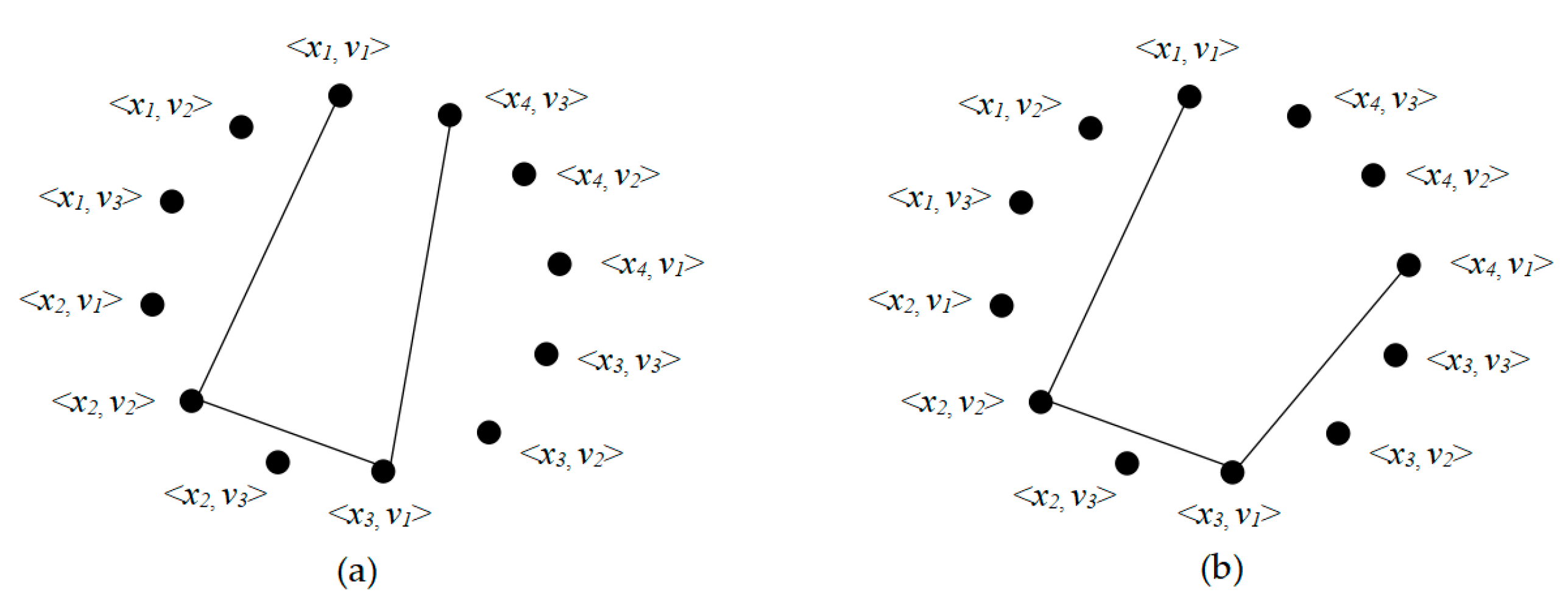
2.1. Problem Definition
2.2. Original Ant Colony Optimization (ACO)
2.3. Ant Colony Optimization Based on Information Entropy (ACOE)
| Algorithm 1 ACOE |
| Input: a CSP (X, D, C), maximum number of iterations Nmax, number of ants Nant |
| Output:bestA |
| 1: Initialization |
| 2: repeat |
| 3: for k = 1 to Nant do |
| 4: Construct a complete assignment Ak |
| 5: if cost(Ak) < cost(bestA) then |
| 6: bestA ← Ak |
| 7: end if |
| 8: if the condition is satisfied then |
| 9: bestA ← CLS(bestA) |
| 10: end if |
| 11: end for |
| 12: Update pheromone on each vertex |
| 13: until cost(bestA) = 0 ∨ Nmax is reached |
| 14: return bestA |
2.3.1. Assignment Construction
| Algorithm 2 Assignment Construction |
| Input: ant k |
| Output:Ak |
| 1: Selects a starting vertex <xi, vp> |
| 2: Place ant k on the vertex <xi, vp> |
| 3: Ak ← <xi, vp> |
| 4: while |Ak| < |X| do |
| 5: Select vertex <xj, vq> that is not assigned to Ak |
| 6: Move ant k to <xj, vq> |
| 7: Ak ← Ak ∪ <xj, vq> |
| 8: end while |
| 9: return Ak |
2.3.2. Ranking-Based Pheromone Updating
2.3.3. Automatic Adjustment Mechanism Based on Information Entropy
2.3.4. Crossover-Based Local Search
| Algorithm 3 CLS |
| Input: bestA, number of crossover operations L, number of values m |
| Output: bestA |
| 1: for u = 1 to L do |
| 2: Au ← select a random assignment |
| 3: crossover point ← U [1, m − 1] |
| 4: C ← Crossover(bestA, Au) |
| 5: if cost(C) < cost(bestA) then |
| 6: bestA ← C |
| 7: end if |
| 8: end for |
| 9: return bestA |
2.3.5. Parameter Setting
3. Results and Discussion
3.1. Datasets
3.2. Cost Comparison
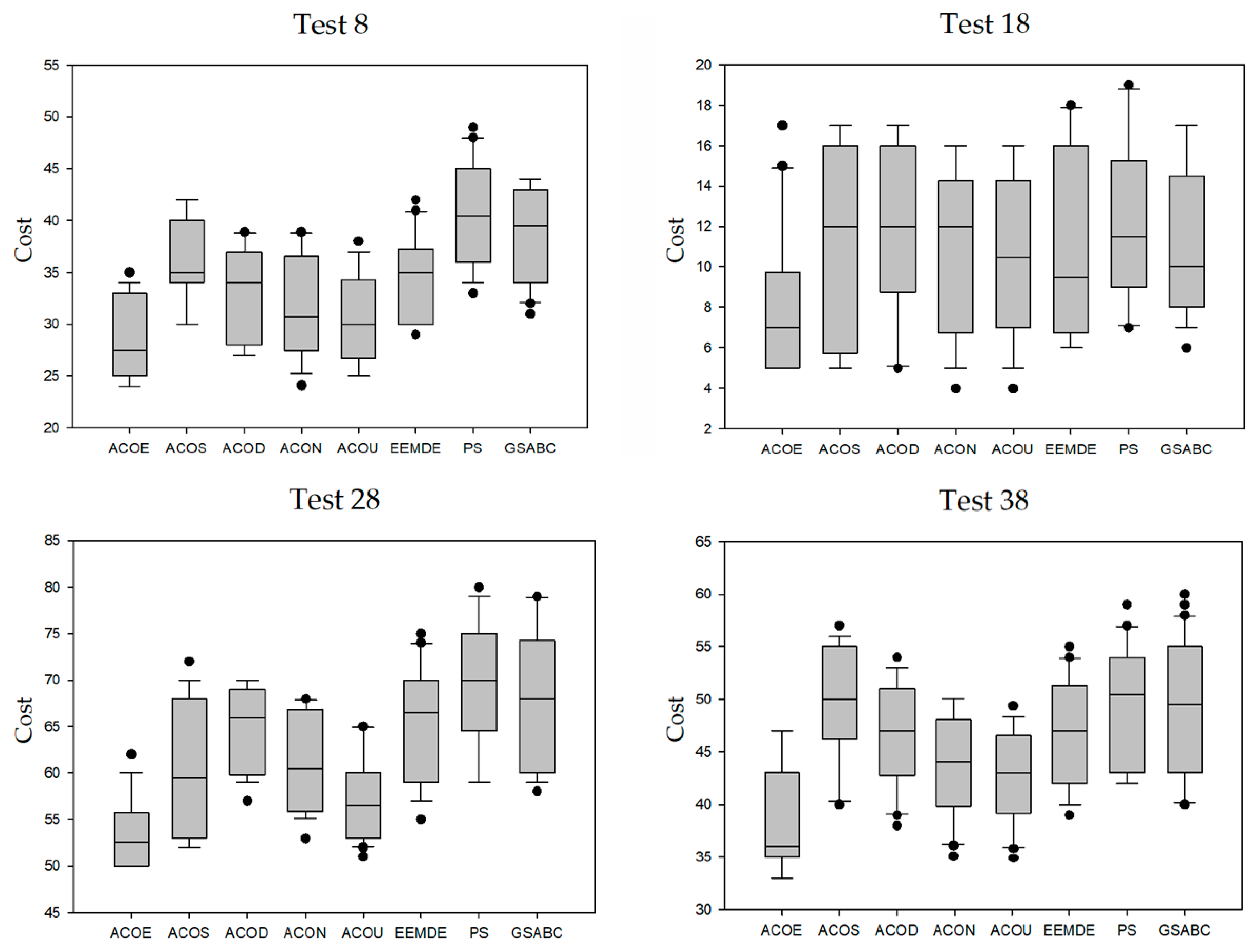
3.3. Result Distribution Analysis
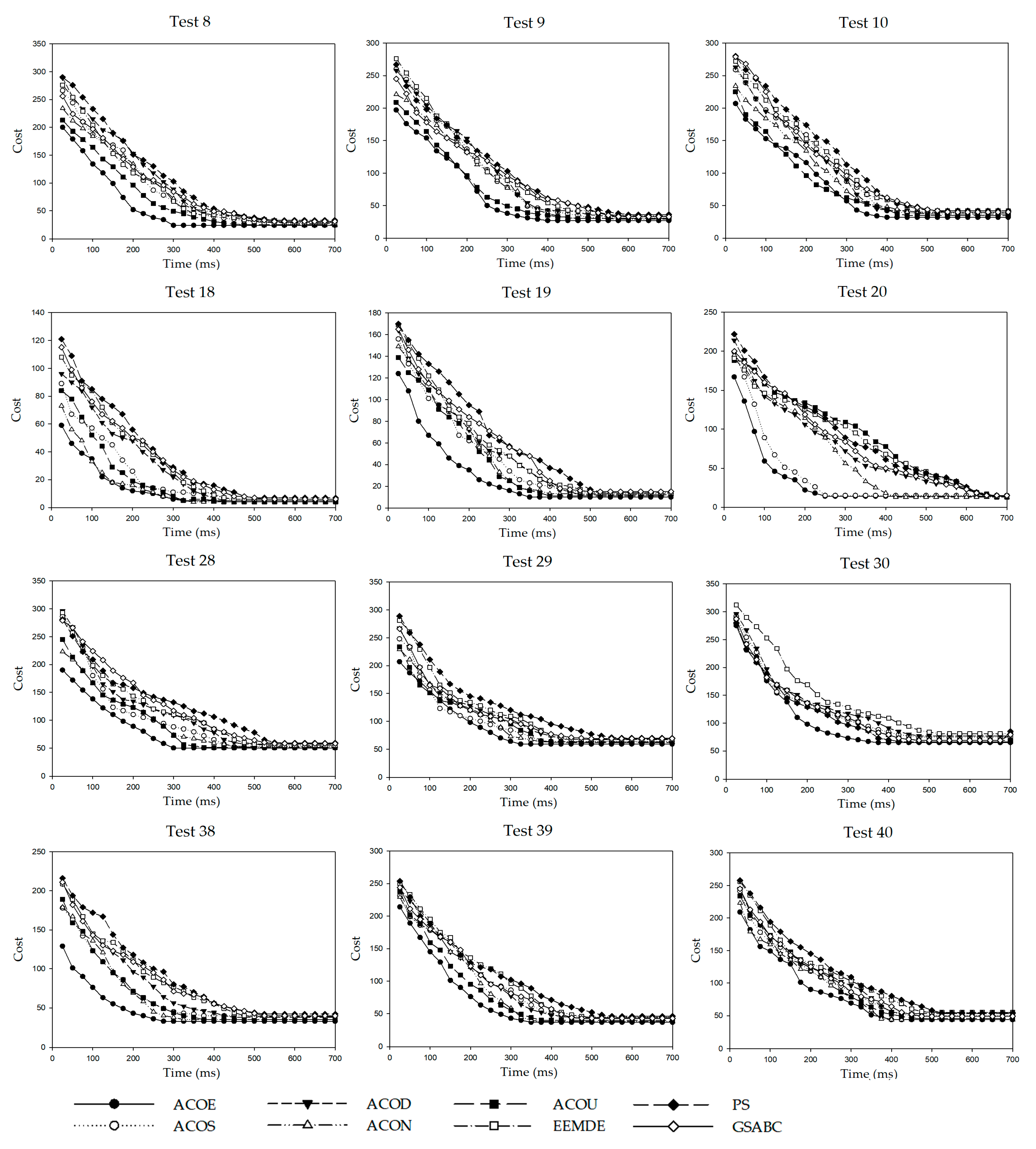
3.4. Convergence Analysis
3.5. Hypothesis Test
4. Conclusions
Author Contributions
Funding
Conflicts of Interest
References
- Bodirsky, M.; Martin, B.; Mottet, A. Discrete temporal constraint satisfaction problems. J. ACM 2018, 65, 1–41. [Google Scholar] [CrossRef]
- Rutishauser, U.; Slotine, J.J.; Douglas, R.J. Solving constraint-satisfaction problems with distributed neocortical-like neuronal networks. Neural Comput. 2018, 30, 1359–1393. [Google Scholar] [CrossRef] [PubMed]
- Yin, B.; Wei, X.; Liu, Y. Finding the most influential product under distribution constraints through dominance tests. Appl. Intell. 2019, 49, 723–740. [Google Scholar] [CrossRef]
- Li, H.; Li, Z. A novel strategy of combining variable ordering heuristics for constraint satisfaction problems. IEEE Access 2018, 6, 42750–42756. [Google Scholar] [CrossRef]
- Xu, W.; Gong, F. Performances of pure random walk algorithms on constraint satisfaction problems with growing domains. J. Comb. Optim. 2016, 32, 51–66. [Google Scholar] [CrossRef]
- Gonzalez-Pardo, A.; Ser, A.J.D.; Camacho, D. Comparative study of pheromone control heuristics in ACO algorithms for solving RCPSP problems. Appl. Soft Comput. 2017, 60, 241–255. [Google Scholar] [CrossRef]
- Bacanin, N.; Tuba, M. Firefly algorithm for cardinality constrained mean-variance portfolio optimization problem with entropy diversity constraint. Sci. World J. 2014, 60, 1–16. [Google Scholar] [CrossRef]
- Strumberger, I.; Minovic, M.; Tuba, M.; Bacanin, N. Performance of elephant herding optimization and tree growth algorithm adapted for node localization in wireless sensor networks. Sensors 2019, 19, 2515. [Google Scholar] [CrossRef]
- Tiwari, P.K.; Vidyarthi, D.P. Improved auto control ant colony optimization using lazy ant approach for grid scheduling problem. Future Gener. Comput. Syst. 2016, 60, 78–89. [Google Scholar] [CrossRef]
- Deng, W.; Xu, J.; Zhao, H. An improved ant colony optimization algorithm based on hybrid strategies for scheduling problem. IEEE Access 2019, 7, 20281–20292. [Google Scholar] [CrossRef]
- Booth, K.E.C.; Tran, T.T.; Nejat, G. Mixed-integer and constraint programming techniques for mobile robot task planning. IEEE Robot. Autom. Lett. 2016, 1, 500–507. [Google Scholar] [CrossRef]
- Deng, W.; Zhang, S.; Zhao, H.; Yang, X. A novel fault diagnosis method based on integrating empirical wavelet transform and fuzzy entropy for motor bearing. IEEE Access 2018, 6, 35042–35056. [Google Scholar] [CrossRef]
- Deng, W.; Zhao, H.; Yang, X.; Xiong, J.; Sun, M.; Li, B. Study on an improved adaptive PSO algorithm for solving multi-objective gate assignment. Appl. Soft Comput. 2017, 59, 288–302. [Google Scholar] [CrossRef]
- Deng, W.; Sun, M.; Zhao, H.; Li, B.; Wang, C. Study on an airport gate assignment method based on improved aco algorithm. Kybernetes 2018, 47, 20–43. [Google Scholar] [CrossRef]
- Paterakis, N.G.; Gibescu, M.; Bakirtzis, A.G.; Catalao, J.P.S. A multi-objective optimization approach to risk-constrained energy and reserve procurement using demand response. IEEE Trans. Power Syst. 2018, 33, 3940–3954. [Google Scholar] [CrossRef]
- Zhao, H.; Yao, R.; Xu, L.; Yuan, Y.; Li, G.; Deng, W. Study on a novel fault damage degree identification method using high-order differential mathematical morphology gradient spectrum entropy. Entropy 2018, 20, 682. [Google Scholar] [CrossRef]
- Wang, H.; Hu, Z.; Sun, Y.; Su, Q.; Xia, X. Modified backtracking search optimization algorithm inspired by simulated annealing for constrained engineering optimization problems. Comput. Intel. Neurosc. 2018, 4, 1–27. [Google Scholar] [CrossRef] [PubMed]
- Zhang, C.; Lin, Q.; Gao, L.; Li, X. Backtracking Search Algorithm with three constraint handling methods for constrained optimization problems. Expert Syst. Appl. 2016, 42, 7831–7845. [Google Scholar] [CrossRef]
- Huss, W.; Levine, L.; Savahuss, E. Interpolating between random walk and rotor walk. Random Struct. Algor. 2018, 52, 263–282. [Google Scholar] [CrossRef]
- Craenen, B.; Eiben, A.; Van Hemert, J. Comparing evolutionary algorithms on binary constraint satisfaction problems. IEEE Trans. Evol. Comput. 2003, 7, 424–444. [Google Scholar] [CrossRef]
- Fu, H. A hybrid differential evolution algorithm for binary csps. Adv. Mater. Res. 2010, 108–111, 328–334. [Google Scholar] [CrossRef]
- Schoofs, L.; Naudts, B. Swarm intelligence on the binary constraint satisfaction problem. In Proceedings of the 2002 Congress on Evolutionary Computation, Honolulu, HI, USA, 12–17 May 2002. [Google Scholar]
- Aratsu, Y.; Mizuno, K.; Sasaki, H.; Nishihara, S. Experimental evaluation of artificial bee colony with greedy scouts for constraint satisfaction problems. In Proceedings of the 2013 Conference on Technologies and Applications of Artificial Intelligence, Taipei, Taiwan, 6–8 December 2013. [Google Scholar]
- Tarrant, F.; Bridge, D. When ants attack: Ant algorithms for constraint satisfaction problems. Artif. Intell. Rev. 2005, 24, 455–476. [Google Scholar] [CrossRef]
- Ye, K.; Zhang, C.; Ning, J.; Liu, X. Ant-colony algorithm with a strengthened negative-feedback mechanism for constraint-satisfaction problems. Inf. Sci. 2017, 406, 29–41. [Google Scholar]
- Zhang, Q.; Zhang, C. An improved ant colony optimization algorithm with strengthened pheromone updating mechanism for constraint satisfaction problem. Neural Comput. Appl. 2017, 1, 1–12. [Google Scholar] [CrossRef]
- Dorigo, M.; Caro, G.D.; Gambardella, L.M. Ant algorithms for discrete optimization. Artif. Intell. 1999, 5, 137–172. [Google Scholar] [CrossRef]
- Stützle, T.; Hoos, H.H. Max-min ant system. J. Future Gener. Comput. Syst. 2000, 16, 889–914. [Google Scholar] [CrossRef]
- Solnon, C. Ants can solve constraint satisfaction problems. IEEE Trans. Evol. Comput. 2002, 6, 347–357. [Google Scholar] [CrossRef]
- Xu, C.; Boussemart, F.; Hemery, F.; Lecoutre, C. Random constraint satisfaction: Easy generation of hard (satisfiable) instances. Artif. Intell. 2007, 171, 514–534. [Google Scholar] [CrossRef]
- Fan, Y.; Shen, J. On the phase transitions of random k-constraint satisfaction problems. Artif. Intell. 2011, 175, 914–927. [Google Scholar] [CrossRef]


| ρ | β | 6 | 8 | 10 | |||||||||
| α | 2 | 3 | 4 | 5 | 2 | 3 | 4 | 5 | 2 | 3 | 4 | 5 | |
| 0.01 | 28 | 26 | 26 | 28 | 25 | 25 | 26 | 27 | 24 | 25 | 25 | 27 | |
| 0.02 | 29 | 30 | 29 | 29 | 26 | 26 | 26 | 28 | 25 | 26 | 25 | 27 | |
| 0.03 | 30 | 31 | 30 | 29 | 26 | 27 | 26 | 27 | 25 | 26 | 26 | 28 | |
| 0.04 | 29 | 30 | 30 | 31 | 28 | 27 | 28 | 29 | 25 | 26 | 27 | 28 | |
| 0.05 | 30 | 29 | 31 | 30 | 27 | 29 | 30 | 31 | 26 | 28 | 30 | 29 | |
| Component Set | Test Case | p2 | k | |
|---|---|---|---|---|
| Class 1 | (100, 4, 0.14, p2) | Test 1 | 0.10 | 0.527 |
| Test 2 | 0.12 | 0.639 | ||
| Test 3 | 0.14 | 0.754 | ||
| Test 4 | 0.16 | 0.872 | ||
| Test 5 | 0.18 | 0.992 | ||
| Test 6 | 0.20 | 1.115 | ||
| Test 7 | 0.22 | 1.242 | ||
| Test 8 | 0.24 | 1.372 | ||
| Test 9 | 0.26 | 1.505 | ||
| Test 10 | 0.28 | 1.642 | ||
| Class 2 | (100, 8, 0.14, p2) | Test 11 | 0.12 | 0.426 |
| Test 12 | 0.14 | 0.503 | ||
| Test 13 | 0.16 | 0.581 | ||
| Test 14 | 0.18 | 0.661 | ||
| Test 15 | 0.20 | 0.743 | ||
| Test 16 | 0.22 | 0.828 | ||
| Test 17 | 0.24 | 0.914 | ||
| Test 18 | 0.26 | 1.003 | ||
| Test 19 | 0.28 | 1.094 | ||
| Test 20 | 0.30 | 1.188 | ||
| Class 3 | (150, 4, 0.14, p2) | Test 21 | 0.06 | 0.466 |
| Test 22 | 0.08 | 0.627 | ||
| Test 23 | 0.10 | 0.793 | ||
| Test 24 | 0.12 | 0.961 | ||
| Test 25 | 0.14 | 1.134 | ||
| Test 26 | 0.16 | 1.311 | ||
| Test 27 | 0.18 | 1.493 | ||
| Test 28 | 0.20 | 1.679 | ||
| Test 29 | 0.22 | 1.869 | ||
| Test 30 | 0.24 | 2.605 | ||
| Class 4 | (150, 8, 0.14, p2) | Test 31 | 0.10 | 0.528 |
| Test 32 | 0.12 | 0.641 | ||
| Test 33 | 0.14 | 0.756 | ||
| Test 34 | 0.16 | 0.874 | ||
| Test 35 | 0.18 | 0.995 | ||
| Test 36 | 0.20 | 1.119 | ||
| Test 37 | 0.22 | 1.246 | ||
| Test 38 | 0.24 | 1.376 | ||
| Test 39 | 0.26 | 1.510 | ||
| Test 40 | 0.28 | 1.648 |
| Minimum Cost/Average Cost/Maximum Cost | ||||||||
|---|---|---|---|---|---|---|---|---|
| Test Case | ACOE | ACOS | ACOD | ACON | ACOU | EEMDE | PS | GSABC |
| Test 1 | 0/0/0 | 0/0/1 | 0/1/1 | 0/0/1 | 0/0/0 | 0/1/2 | 0/1/1 | 0/0/1 |
| Test 2 | 0/0/1 | 0/1/2 | 0/1/2 | 0/0/1 | 0/1/1 | 0/0/1 | 0/1/2 | 0/1/2 |
| Test 3 | 0/0/1 | 0/1/4 | 0/1/2 | 0/1/2 | 0/1/2 | 0/2/3 | 1/2/4 | 1/1/3 |
| Test 4 | 0/0/2 | 0/2/5 | 0/1/3 | 0/1/3 | 0/0/2 | 0/2/3 | 0/2/4 | 0/1/2 |
| Test 5 | 0/0/1 | 0/1/3 | 0/1/3 | 0/0/2 | 0/1/2 | 0/1/2 | 1/2/3 | 0/1/2 |
| Test 6 | 0/2/4 | 0/4/6 | 0/5/8 | 0/3/5 | 0/3/4 | 0/4/7 | 1/4/6 | 1/3/5 |
| Test 7 | 24/30/38 | 29/35/42 | 29/34/39 | 27/35/40 | 25/32/39 | 28/37/45 | 30/38/46 | 27/36/41 |
| Test 8 | 24/28/35 | 30/37/42 | 27/32/39 | 24/33/39 | 25/31/38 | 29/36/42 | 33/40/49 | 31/38/44 |
| Test 9 | 27/34/41 | 31/40/47 | 33/42/47 | 29/36/43 | 30/36/46 | 34/42/48 | 36/42/50 | 33/41/46 |
| Test 10 | 32/39/45 | 39/48/54 | 40/48/47 | 37/43/49 | 35/39/48 | 42/50/57 | 42/52/59 | 40/46/53 |
| Test 11 | 0/1/1 | 0/1/3 | 0/1/2 | 0/1/2 | 0/1/2 | 0/1/3 | 0/2/4 | 0/1/2 |
| Test 12 | 0/2/4 | 1/3/5 | 0/3/5 | 0/3/4 | 0/2/5 | 1/3/6 | 2/4/7 | 0/3/6 |
| Test 13 | 0/4/6 | 1/5/7 | 1/5/8 | 0/5/7 | 0/4/7 | 1/4/8 | 1/5/9 | 1/5/8 |
| Test 14 | 1/4/7 | 2/6/9 | 2/8/10 | 1/4/8 | 1/5/10 | 2/7/11 | 3/8/12 | 2/8/11 |
| Test 15 | 0/5/7 | 1/6/10 | 0/5/10 | 0/5/9 | 0/5/8 | 1/6/10 | 1/6/11 | 1/5/10 |
| Test 16 | 0/6/9 | 2/8/10 | 2/9/12 | 1/8/12 | 1/7/12 | 3/9/13 | 3/10/14 | 2/9/13 |
| Test 17 | 3/8/14 | 5/10/18 | 4/10/16 | 4/9/15 | 4/10/15 | 5/11/16 | 6/12/19 | 5/11/18 |
| Test 18 | 5/8/17 | 5/11/17 | 5/10/17 | 4/10/16 | 5/9/16 | 6/9/18 | 7/11/19 | 6/10/17 |
| Test 19 | 10/15/24 | 14/19/25 | 12/18/25 | 13/17/24 | 11/17/25 | 14/19/27 | 15/19/29 | 15/18/26 |
| Test 20 | 14/18/24 | 15/20/27 | 14/21/29 | 13/20/28 | 13/19/27 | 16/21/31 | 17/23/32 | 17/21/30 |
| Test 21 | 3/4/7 | 4/7/10 | 5/7/9 | 3/5/7 | 3/5/8 | 5/8/10 | 6/10/14 | 6/8/11 |
| Test 22 | 5/6/11 | 7/9/12 | 7/10/14 | 6/9/14 | 7/10/13 | 9/13/17 | 9/13/19 | 8/12/16 |
| Test 23 | 6/8/13 | 7/11/15 | 7/10/15 | 6/10/14 | 6/11/14 | 8/12/17 | 8/14/19 | 7/12/16 |
| Test 24 | 6/9/13 | 8/12/16 | 7/12/16 | 8/12/15 | 7/11/15 | 9/13/18 | 11/15/20 | 8/14/19 |
| Test 25 | 5/8/14 | 6/12/16 | 5/11/16 | 5/10/15 | 6/11/16 | 8/13/18 | 10/15/19 | 6/13/17 |
| Test 26 | 24/33/41 | 28/40/45 | 27/39/45 | 26/38/44 | 27/39/42 | 31/42/49 | 33/45/52 | 29/41/48 |
| Test 27 | 53/57/63 | 57/65/73 | 59/64/72 | 56/62/70 | 56/61/72 | 60/68/78 | 65/74/85 | 61/70/83 |
| Test 28 | 50/52/62 | 52/65/72 | 57/64/70 | 53/60/68 | 51/59/65 | 55/66/75 | 59/69/80 | 58/67/79 |
| Test 29 | 59/69/77 | 64/75/87 | 68/77/88 | 63/70/80 | 62/71/83 | 67/78/90 | 70/82/95 | 69/80/92 |
| Test 30 | 65/73/84 | 75/83/94 | 77/89/95 | 66/75/87 | 69/76/89 | 81/95/105 | 85/98/105 | 79/92/98 |
| Test 31 | 0/0/0 | 0/0/2 | 0/1/2 | 0/0/1 | 0/0/2 | 0/1/3 | 0/1/2 | 0/1/3 |
| Test 32 | 0/1/2 | 2/4/5 | 1/3/4 | 0/1/3 | 0/2/3 | 2/4/6 | 3/5/6 | 2/3/5 |
| Test 33 | 0/2/4 | 2/4/7 | 2/4/6 | 1/3/4 | 2/3/5 | 2/5/8 | 3/6/8 | 2/3/6 |
| Test 34 | 1/3/6 | 2/5/8 | 2/5/8 | 2/4/7 | 2/4/8 | 3/5/9 | 3/6/10 | 2/5/9 |
| Test 35 | 1/3/8 | 2/6/11 | 2/6/10 | 1/5/10 | 2/5/10 | 2/7/11 | 3/9/14 | 2/7/10 |
| Test 36 | 22/27/32 | 25/32/39 | 25/30/36 | 24/30/34 | 24/29/34 | 29/36/43 | 31/39/48 | 30/38/45 |
| Test 37 | 29/33/45 | 34/41/54 | 35/40/52 | 33/38/47 | 33/39/49 | 38/45/57 | 40/47/63 | 35/45/54 |
| Test 38 | 33/40/47 | 40/51/57 | 38/47/54 | 35/43/49 | 35/42/48 | 39/49/55 | 42/50/59 | 40/49/60 |
| Test 39 | 37/45/52 | 45/53/60 | 44/54/59 | 38/48/54 | 40/47/56 | 44/55/61 | 46/58/69 | 43/56/62 |
| Test 40 | 44/49/57 | 50/59/66 | 53/60/68 | 44/50/59 | 46/52/61 | 55/64/73 | 54/68/78 | 49/59/70 |
| Test Case | ACOE | ACOS | ACOD | ACON | ACOU | EEMDE | PS | GSABC | |
|---|---|---|---|---|---|---|---|---|---|
| Test 1 | ACOE | – | 0.438 | 0.402 | 0.443 | 0.500 | 0.385 | 0.419 | 0.440 |
| ACOS | 0.568 | – | 0.496 | 0.536 | 0.568 | 0.423 | 0.439 | 0.560 | |
| ACOD | 0.598 | 0.504 | – | 0.573 | 0.598 | 0.434 | 0.503 | 0.569 | |
| ACON | 0.557 | 0.464 | 0.427 | – | 0.557 | 0.401 | 0.435 | 0.494 | |
| ACOU | 0.500 | 0.432 | 0.402 | 0.443 | – | 0.385 | 0.419 | 0.440 | |
| EEMDE | 0.615 | 0.577 | 0.566 | 0.599 | 0.615 | – | 0.579 | 0.595 | |
| PS | 0.581 | 0.561 | 0.497 | 0.565 | 0.581 | 0.421 | – | 0.562 | |
| GSABC | 0.560 | 0.440 | 0.431 | 0.506 | 0.560 | 0.405 | 0.438 | – | |
| Test 2 | ACOE | – | 0.321 | 0.315 | 0.440 | 0.380 | 0.436 | 0.309 | 0.298 |
| ACOS | 0.679 | – | 0.480 | 0.624 | 0.604 | 0.610 | 0.472 | 0.465 | |
| ACOD | 0.685 | 0.520 | – | 0.638 | 0.609 | 0.617 | 0.477 | 0.470 | |
| ACON | 0.560 | 0.376 | 0.362 | – | 0.419 | 0.466 | 0.355 | 0.350 | |
| ACOU | 0.620 | 0.396 | 0.391 | 0.581 | – | 0.511 | 0.384 | 0.376 | |
| EEMDE | 0.564 | 0.390 | 0.383 | 0.534 | 0.489 | – | 0.375 | 0.369 | |
| PS | 0.691 | 0.528 | 0.527 | 0.645 | 0.616 | 0.625 | – | 0.481 | |
| GSABC | 0.702 | 0.535 | 0.530 | 0.650 | 0.624 | 0.631 | 0.519 | – | |
| Test 3 | ACOE | – | 0.303 | 0.347 | 0.398 | 0.465 | 0.067 | 7.890 × 10⁻⁴ | 0.187 |
| ACOS | 0.697 | – | 0.580 | 0.589 | 0.598 | 0.214 | 0.177 | 0.323 | |
| ACOD | 0.653 | 0.420 | – | 0.508 | 0.531 | 0.151 | 0.104 | 0.278 | |
| ACON | 0.602 | 0.411 | 0.492 | – | 0.517 | 0.143 | 0.097 | 0.271 | |
| ACOU | 0.535 | 0.402 | 0.469 | 0.483 | – | 0.128 | 0.088 | 0.255 | |
| EEMDE | 0.933 | 0.786 | 0.849 | 0.857 | 0.878 | – | 0.378 | 0.667 | |
| PS | 1 | 0.823 | 0.896 | 0.903 | 0.912 | 0.222 | – | 0.791 | |
| GSABC | 0.813 | 0.677 | 0.722 | 0.729 | 0.745 | 0.333 | 0.209 | – | |
| Test 4 | ACOE | – | 0.005 | 0.244 | 0.240 | 0.330 | 0.103 | 0.045 | 0.309 |
| ACOS | 0.995 | – | 0.874 | 0.865 | 0.945 | 0.708 | 0.665 | 0.901 | |
| ACOD | 0.756 | 0.126 | – | 0.487 | 0.711 | 0.288 | 0.279 | 0.663 | |
| ACON | 0.760 | 0.135 | 0.513 | – | 0.720 | 0.296 | 0.290 | 0.669 | |
| ACOU | 0.670 | 0.055 | 0.289 | 0.280 | – | 0.195 | 0.102 | 0.389 | |
| EEMDE | 0.897 | 0.292 | 0.712 | 0.704 | 0.805 | – | 0.388 | 0.789 | |
| PS | 0.955 | 0.335 | 0.721 | 0.710 | 0.898 | 0.612 | – | 0.833 | |
| GSABC | 0.691 | 0.099 | 0.337 | 0.331 | 0.611 | 0.211 | 0.167 | – | |
| Test 5 | ACOE | – | 0.209 | 0.201 | 0.400 | 0.353 | 0.348 | 0.122 | 0.341 |
| ACOS | 0.791 | – | 0.458 | 0.681 | 0.620 | 0.612 | 0.366 | 0.605 | |
| ACOD | 0.799 | 0.542 | – | 0.688 | 0.623 | 0.618 | 0.397 | 0.610 | |
| ACON | 0.600 | 0.319 | 0.312 | – | 0.476 | 0.470 | 0.209 | 0.465 | |
| ACOU | 0.647 | 0.380 | 0.377 | 0.524 | – | 0.495 | 0.298 | 0.491 | |
| EEMDE | 0.652 | 0.388 | 0.382 | 0.530 | 0.505 | – | 0.312 | 0.498 | |
| PS | 0.878 | 0.644 | 0.603 | 0.791 | 0.702 | 0.668 | – | 0.679 | |
| GSABC | 0.659 | 0.395 | 0.390 | 0.535 | 0.509 | 0.508 | 0.321 | – | |
| Test 6 | ACOE | – | 0.038 | 7.765 × 10⁻⁵ | 0.114 | 0.266 | 6.742 × 10⁻⁴ | 6.009 × 10⁻⁴ | 0.043 |
| ACOS | 0.962 | – | 0.102 | 0.777 | 0.891 | 0.289 | 0.276 | 0.691 | |
| ACOD | 1 | 0.898 | – | 0.991 | 1 | 0.792 | 0.660 | 0.945 | |
| ACON | 0.886 | 0.223 | 0.009 | – | 0.768 | 0.067 | 0.059 | 0.290 | |
| ACOU | 0.734 | 0.109 | 8.789 × 10⁻⁴ | 0.232 | – | 0.009 | 0.007 | 0.176 | |
| EEMDE | 1 | 0.711 | 0.208 | 0.933 | 0.991 | – | 0.355 | 0.887 | |
| PS | 1 | 0.724 | 0.340 | 0.941 | 0.993 | 0.645 | – | 0.892 | |
| GSABC | 0.957 | 0.309 | 0.055 | 0.710 | 0.824 | 0.113 | 0.108 | – | |
| Test 7 | ACOE | – | 0.039 | 0.165 | 0.045 | 0.389 | 1.335 × 10⁻⁴ | 1.004 × 10⁻⁶ | 9.876 × 10⁻⁴ |
| ACOS | 0.961 | – | 0.858 | 0.720 | 0.933 | 0.221 | 0.115 | 0.290 | |
| ACOD | 0.835 | 0.142 | – | 0.419 | 0.776 | 0.009 | 0.001 | 0.067 | |
| ACON | 0.955 | 0.280 | 0.581 | – | 0.895 | 0.113 | 0.062 | 0.182 | |
| ACOU | 0.611 | 0.067 | 0.224 | 0.105 | – | 8.884 × 10⁻⁴ | 1.453 × 10⁻⁴ | 0.008 | |
| EEMDE | 1 | 0.779 | 0.991 | 0.887 | 1 | – | 0.399 | 0.662 | |
| PS | 1 | 0.885 | 0.999 | 0.938 | 1 | 0.601 | – | 0.794 | |
| GSABC | 1 | 0.710 | 0.933 | 0.818 | 0.992 | 0.338 | 0.206 | – | |
| Test 8 | ACOE | – | 7.542 × 10⁻⁴ | 0.009 | 0.019 | 0.025 | 0.001 | 7.544 × 10⁻⁸ | 5.980 × 10⁻⁶ |
| ACOS | 1 | – | 0.595 | 0.634 | 0.809 | 0.553 | 0.167 | 0.225 | |
| ACOD | 0.991 | 0.405 | – | 0.562 | 0.622 | 0.444 | 0.004 | 0.027 | |
| ACON | 0.981 | 0.366 | 0.432 | – | 0.560 | 0.408 | 6.669 × 10⁻⁴ | 0.004 | |
| ACOU | 0.975 | 0.191 | 0.388 | 0.440 | – | 0.208 | 7.664 × 10⁻⁵ | 6.659 × 10⁻⁴ | |
| EEMDE | 0.999 | 0.447 | 0.556 | 0.592 | 0.798 | – | 0.096 | 0.122 | |
| PS | 1 | 0.833 | 0.996 | 1 | 1 | 0.904 | – | 0.726 | |
| GSABC | 1 | 0.775 | 0.973 | 0.996 | 1 | 0.878 | 0.274 | – | |
| Test 9 | ACOE | – | 0.004 | 5.545 × 10⁻⁷ | 0.054 | 0.029 | 5.898 × 10⁻⁸ | 7.653 × 10⁻⁹ | 6.645 × 10⁻⁶ |
| ACOS | 0.996 | – | 0.005 | 0.913 | 0.834 | 7.706 × 10⁻⁵ | 8.744 × 10⁻⁶ | 0.012 | |
| ACOD | 1 | 0.995 | – | 1 | 1 | 0.004 | 1.975 × 10⁻⁴ | 0.992 | |
| ACON | 0.946 | 0.087 | 4.655 × 10⁻⁶ | – | 0.355 | 2.670 × 10⁻⁷ | 7.980 × 10⁻⁸ | 7.707 × 10⁻⁵ | |
| ACOU | 0.971 | 0.166 | 1.542 × 10⁻⁴ | 0.645 | – | 9.994 × 10⁻⁶ | 1.325 × 10⁻⁶ | 9.966 × 10⁻⁴ | |
| EEMDE | 1 | 1 | 0.996 | 1 | 1 | – | 0.238 | 1 | |
| PS | 1 | 1 | 1 | 1 | 1 | 0.762 | – | 1 | |
| GSABC | 1 | 0.988 | 0.008 | 1 | 1 | 9.642 × 10⁻⁴ | 1.565 × 10⁻⁴ | – | |
| Test 10 | ACOE | – | 1.222 × 10⁻⁵ | 9.667 × 10⁻⁵ | 4.448 × 10⁻⁴ | 0.007 | 8.890 × 10⁻⁸ | 3.897 × 10⁻¹⁰ | 8.754 × 10⁻⁷ |
| ACOS | 1 | – | 1 | 1 | 1 | 2.238 × 10⁻⁵ | 9.688 × 10⁻⁷ | 9.998 × 10⁻⁵ | |
| ACOD | 1 | 7.766 × 10⁻⁴ | – | 0.993 | 1 | 8.890 × 10⁻⁶ | 3.346 × 10⁻⁷ | 2.346 × 10⁻⁵ | |
| ACON | 1 | 9.986 × 10⁻⁵ | 0.007 | – | 0.995 | 1.565 × 10⁻⁶ | 8.853 × 10⁻⁸ | 8.785 × 10⁻⁶ | |
| ACOU | 0.993 | 1.867 × 10⁻⁵ | 8.855 × 10⁻⁴ | 0.005 | – | 9.909 × 10⁻⁷ | 6.678 × 10⁻⁹ | 3.332 × 10⁻⁶ | |
| EEMDE | 1 | 1 | 1 | 1 | 1 | – | 0.998 | 1 | |
| PS | 1 | 1 | 1 | 1 | 1 | 0.002 | – | 1 | |
| GSABC | 1 | 1 | 1 | 1 | 1 | 5.323 × 10⁻⁴ | 4.455 × 10⁻⁵ | – | |
| Test 11 | ACOE | – | 0.185 | 0.206 | 0.295 | 0.310 | 0.182 | 7.656 × 10⁻⁵ | 0.203 |
| ACOS | 0.815 | – | 0.558 | 0.688 | 0.756 | 0.397 | 0.234 | 0.502 | |
| ACOD | 0.794 | 0.442 | – | 0.597 | 0.698 | 0.335 | 0.008 | 0.490 | |
| ACON | 0.705 | 0.312 | 0.403 | – | 0.603 | 0.306 | 2.276 × 10⁻⁴ | 0.391 | |
| ACOU | 0.690 | 0.244 | 0.302 | 0.397 | – | 0.239 | 8.645 × 10⁻⁴ | 0.295 | |
| EEMDE | 0.818 | 0.603 | 0.665 | 0.694 | 0.761 | – | 0.245 | 0.610 | |
| PS | 1 | 0.766 | 0.992 | 1 | 1 | 0.755 | – | 0.873 | |
| GSABC | 0.797 | 0.498 | 0.510 | 0.609 | 0.705 | 0.390 | 0.127 | – | |
| Test 12 | ACOE | – | 0.156 | 0.256 | 0.320 | 0.355 | 0.002 | 5.895 × 10⁻⁴ | 0.036 |
| ACOS | 0.844 | – | 0.560 | 0.599 | 0.635 | 0.387 | 0.324 | 0.425 | |
| ACOD | 0.744 | 0.440 | – | 0.552 | 0.580 | 0.345 | 0.303 | 0.398 | |
| ACON | 0.680 | 0.401 | 0.448 | – | 0.511 | 0.297 | 0.276 | 0.345 | |
| ACOU | 0.645 | 0.365 | 0.420 | 0.489 | – | 0.189 | 0.180 | 0.267 | |
| EEMDE | 0.998 | 0.613 | 0.655 | 0.703 | 0.811 | – | 0.458 | 0.582 | |
| PS | 1 | 0.676 | 0.697 | 0.724 | 0.820 | 0.542 | – | 0.604 | |
| GSABC | 0.964 | 0.575 | 0.602 | 0.655 | 0.733 | 0.418 | 0.396 | – | |
| Test 13 | ACOE | – | 0.041 | 0.026 | 0.207 | 0.290 | 0.037 | 6.766 × 10⁻⁴ | 0.025 |
| ACOS | 0.959 | – | 0.208 | 0.751 | 0.876 | 0.309 | 0.220 | 0.201 | |
| ACOD | 0.974 | 0.792 | – | 0.832 | 0.902 | 0.633 | 0.315 | 0.508 | |
| ACON | 0.793 | 0.249 | 0.168 | – | 0.699 | 0.213 | 0.043 | 0.164 | |
| ACOU | 0.710 | 0.124 | 0.098 | 0.301 | – | 0.117 | 1.006 × 10⁻⁴ | 0.095 | |
| EEMDE | 0.963 | 0.691 | 0.367 | 0.787 | 0.883 | – | 0.279 | 0.361 | |
| PS | 1 | 0.780 | 0.685 | 0.957 | 1 | 0.721 | – | 0.681 | |
| GSABC | 0.975 | 0.799 | 0.498 | 0.836 | 0.905 | 0.639 | 0.319 | – | |
| Test 14 | ACOE | – | 0.027 | 0.009 | 0.176 | 0.055 | 8.560 × 10⁻⁴ | 6.745 × 10⁻⁵ | 1.875 × 10⁻⁴ |
| ACOS | 0.973 | – | 0.277 | 0.658 | 0.511 | 0.149 | 0.011 | 0.085 | |
| ACOD | 0.991 | 0.723 | – | 0.775 | 0.733 | 0.256 | 0.095 | 0.156 | |
| ACON | 0.824 | 0.342 | 0.225 | – | 0.421 | 0.067 | 7.790 × 10⁻⁴ | 0.006 | |
| ACOU | 0.945 | 0.489 | 0.267 | 0.579 | – | 0.144 | 0.009 | 0.078 | |
| EEMDE | 1 | 0.851 | 0.744 | 0.933 | 0.856 | – | 0.243 | 0.387 | |
| PS | 1 | 0.989 | 0.905 | 1 | 0.991 | 0.757 | – | 0.612 | |
| GSABC | 1 | 0.915 | 0.844 | 0.994 | 0.922 | 0.613 | 0.388 | – | |
| Test 15 | ACOE | – | 0.005 | 0.009 | 0.030 | 0.045 | 2.674 × 10⁻⁴ | 6.745 × 10⁻⁵ | 0.006 |
| ACOS | 0.995 | – | 0.560 | 0.714 | 0.993 | 0.379 | 0.204 | 0.507 | |
| ACOD | 0.991 | 0.440 | – | 0.665 | 0.898 | 0.125 | 0.055 | 0.465 | |
| ACON | 0.970 | 0.286 | 0.335 | – | 0.614 | 0.048 | 6.443 × 10⁻⁴ | 0.298 | |
| ACOU | 0.955 | 0.007 | 0.102 | 0.386 | – | 7.888 × 10⁻⁴ | 1.999 × 10⁻⁵ | 0.008 | |
| EEMDE | 1 | 0.621 | 0.875 | 0.952 | 1 | – | 0.499 | 0.632 | |
| PS | 1 | 0.796 | 0.945 | 1 | 1 | 0.501 | – | 0.804 | |
| GSABC | 0.994 | 0.495 | 0.535 | 0.702 | 0.992 | 0.368 | 0.196 | – | |
| Test 16 | ACOE | – | 0.018 | 6.232 × 10⁻⁸ | 5.178 × 10⁻⁷ | 4.181 × 10⁻⁶ | 1.455 × 10⁻⁹ | 5.743 × 10⁻¹⁰ | 8.823 × 10⁻⁹ |
| ACOS | 0.982 | – | 0.013 | 0.024 | 0.031 | 4.532 × 10⁻⁶ | 1.094 × 10⁻⁷ | 7.895 × 10⁻⁶ | |
| ACOD | 1 | 0.987 | – | 0.510 | 0.528 | 7.890 × 10⁻⁴ | 8.643 × 10⁻⁵ | 0.012 | |
| ACON | 1 | 0.976 | 0.490 | – | 0.615 | 1.658 × 10⁻⁴ | 1.005 × 10⁻⁵ | 7.666 × 10⁻⁴ | |
| ACOU | 1 | 0.969 | 0.472 | 0.385 | – | 1.005 × 10⁻⁵ | 8.865 × 10⁻⁶ | 3.077 × 10⁻⁵ | |
| EEMDE | 1 | 1 | 1 | 1 | 1 | – | 0.411 | 0.624 | |
| PS | 1 | 1 | 1 | 1 | 1 | 0.589 | – | 1 | |
| GSABC | 1 | 1 | 0.988 | 1 | 1 | 0.376 | 5.565 × 10⁻⁴ | – | |
| Test 17 | ACOE | – | 5.167 × 10⁻⁸ | 3.344 × 10⁻⁸ | 6.437 × 10⁻⁵ | 8.222 × 10⁻⁴ | 5.543 × 10⁻⁹ | 8.644 × 10⁻¹¹ | 3.534 × 10⁻¹⁰ |
| ACOS | 1 | – | 0.604 | 0.951 | 1 | 0.401 | 0.087 | 0.176 | |
| ACOD | 1 | 0.396 | – | 0.940 | 1 | 0.287 | 8.766 × 10⁻⁴ | 0.005 | |
| ACON | 1 | 0.049 | 0.060 | – | 0.998 | 0.202 | 1.678 × 10⁻⁴ | 7.748 × 10⁻⁴ | |
| ACOU | 1 | 7.892 × 10⁻⁵ | 3.156 × 10⁻⁵ | 0.002 | – | 2.453 × 10⁻⁶ | 1.870 × 10⁻⁷ | 7.655 × 10⁻⁷ | |
| EEMDE | 1 | 0.599 | 0.713 | 0.798 | 1 | – | 0.226 | 0.314 | |
| PS | 1 | 0.913 | 1 | 1 | 1 | 0.774 | – | 0.488 | |
| GSABC | 1 | 0.824 | 0.995 | 1 | 1 | 0.686 | 0.512 | – | |
| Test 18 | ACOE | – | 0.140 | 0.243 | 0.399 | 0.591 | 0.005 | 4.886 × 10⁻⁴ | 0.001 |
| ACOS | 0.860 | – | 0.560 | 0.702 | 0.874 | 0.254 | 0.108 | 0.164 | |
| ACOD | 0.757 | 0.440 | – | 0.631 | 0.798 | 0.120 | 0.067 | 0.096 | |
| ACON | 0.601 | 0.298 | 0.369 | – | 0.613 | 0.057 | 0.006 | 0.012 | |
| ACOU | 0.409 | 0.126 | 0.202 | 0.387 | – | 9.653 × 10⁻⁴ | 1.654 × 10⁻⁴ | 8.953 × 10⁻⁴ | |
| EEMDE | 0.995 | 0.746 | 0.880 | 0.943 | 1 | – | 0.237 | 0.316 | |
| PS | 1 | 0.892 | 0.933 | 0.994 | 1 | 0.763 | – | 0.590 | |
| GSABC | 0.999 | 0.836 | 0.904 | 0.988 | 1 | 0.684 | 0.410 | – | |
| Test 19 | ACOE | – | 0.020 | 0.029 | 0.227 | 0.038 | 1.887 × 10⁻⁵ | 6.673 × 10⁻⁷ | 3.572 × 10⁻⁵ |
| ACOS | 0.980 | – | 0.515 | 0.801 | 0.675 | 0.208 | 0.008 | 0.399 | |
| ACOD | 0.971 | 0.485 | – | 0.768 | 0.508 | 0.058 | 9.777 × 10⁻⁴ | 0.168 | |
| ACON | 0.773 | 0.199 | 0.232 | – | 0.435 | 6.330 × 10⁻⁴ | 8.545 × 10⁻⁵ | 0.008 | |
| ACOU | 0.962 | 0.325 | 0.402 | 0.565 | – | 9.565 × 10⁻⁴ | 2.446 × 10⁻⁴ | 0.043 | |
| EEMDE | 1 | 0.792 | 0.942 | 1 | 1 | – | 0.376 | 0.605 | |
| PS | 1 | 0.992 | 1 | 1 | 1 | 0.624 | – | 0.875 | |
| GSABC | 1 | 0.601 | 0.832 | 0.992 | 0.957 | 0.395 | 0.125 | – | |
| Test 20 | ACOE | – | 0.355 | 0.433 | 0.452 | 0.518 | 0.014 | 6.674 × 10⁻⁴ | 0.003 |
| ACOS | 0.645 | – | 0.577 | 0.600 | 0.773 | 0.276 | 0.168 | 0.201 | |
| ACOD | 0.567 | 0.423 | – | 0.525 | 0.697 | 0.188 | 0.079 | 0.107 | |
| ACON | 0.548 | 0.400 | 0.475 | – | 0.640 | 0.098 | 0.007 | 0.056 | |
| ACOU | 0.482 | 0.227 | 0.303 | 0.360 | – | 0.005 | 8.775 × 10⁻⁵ | 7.653 × 10⁻⁴ | |
| EEMDE | 0.986 | 0.724 | 0.812 | 0.902 | 0.995 | – | 0.288 | 0.316 | |
| PS | 1 | 0.832 | 0.921 | 0.993 | 1 | 0.712 | – | 0.664 | |
| GSABC | 0.997 | 0.799 | 0.893 | 0.944 | 1 | 0.684 | 0.336 | – | |
| Test 21 | ACOE | – | 0.027 | 0.031 | 0.047 | 0.042 | 7.534 × 10⁻⁴ | 5.909 × 10⁻⁶ | 1.166 × 10⁻⁵ |
| ACOS | 0.973 | – | 0.599 | 0.868 | 0.772 | 0.245 | 0.023 | 0.086 | |
| ACOD | 0.969 | 0.401 | – | 0.763 | 0.648 | 0.196 | 0.002 | 0.011 | |
| ACON | 0.953 | 0.132 | 0.237 | – | 0.336 | 0.055 | 9.922 × 10⁻⁵ | 4.542 × 10⁻⁴ | |
| ACOU | 0.958 | 0.228 | 0.352 | 0.664 | – | 0.105 | 1.005 × 10⁻⁴ | 9.965 × 10⁻⁴ | |
| EEMDE | 1 | 0.755 | 0.804 | 0.945 | 0.895 | – | 0.198 | 0.344 | |
| PS | 1 | 0.977 | 0.998 | 1 | 1 | 0.802 | – | 0.602 | |
| GSABC | 1 | 0.914 | 0.989 | 1 | 1 | 0.656 | 0.398 | – | |
| Test 22 | ACOE | – | 0.034 | 0.021 | 0.037 | 0.028 | 1.301 × 10⁻⁵ | 6.446 × 10⁻⁶ | 5.655 × 10⁻⁵ |
| ACOS | 0.966 | – | 0.206 | 0.697 | 0.390 | 0.134 | 0.054 | 0.237 | |
| ACOD | 0.979 | 0.794 | – | 0.875 | 0.630 | 0.303 | 0.256 | 0.379 | |
| ACON | 0.963 | 0.303 | 0.125 | – | 0.134 | 1.050 × 10⁻⁴ | 0.005 | 8.659 × 10⁻⁴ | |
| ACOU | 0.972 | 0.610 | 0.370 | 0.866 | – | 0.201 | 0.118 | 0.298 | |
| EEMDE | 1 | 0.866 | 0.697 | 1 | 0.799 | – | 0.406 | 0.611 | |
| PS | 1 | 0.946 | 0.744 | 0.995 | 0.892 | 0.594 | – | 0.689 | |
| GSABC | 1 | 0.763 | 0.621 | 1 | 0.702 | 0.389 | 0.311 | – | |
| Test 23 | ACOE | – | 5.127 × 10⁻⁷ | 3.654 × 10⁻⁶ | 6.008 × 10⁻⁵ | 5.945 × 10⁻⁵ | 1.334 × 10⁻⁹ | 8.644 × 10⁻¹¹ | 6.523 × 10⁻⁹ |
| ACOS | 1 | – | 0.630 | 0.883 | 0.752 | 0.002 | 7.674 × 10⁻⁴ | 0.008 | |
| ACOD | 1 | 0.370 | – | 0.765 | 0.611 | 1.004 × 10⁻⁴ | 6.653 × 10⁻⁵ | 8.653 × 10⁻⁴ | |
| ACON | 1 | 0.117 | 0.235 | – | 0.380 | 6.678 × 10⁻⁸ | 2.228 × 10⁻⁹ | 6.989 × 10⁻⁷ | |
| ACOU | 1 | 0.242 | 0.389 | 0.620 | – | 5.809 × 10⁻⁶ | 7.787 × 10⁻⁷ | 8.542 × 10⁻⁵ | |
| EEMDE | 1 | 1 | 1 | 1 | 1 | – | 0.249 | 0.562 | |
| PS | 1 | 1 | 1 | 1 | 1 | 0.751 | – | 0.957 | |
| GSABC | 1 | 1 | 1 | 1 | 1 | 0.438 | 0.043 | – | |
| Test 24 | ACOE | – | 9.878 × 10⁻⁶ | 2.289 × 10⁻⁶ | 8.254 × 10⁻⁵ | 2.634 × 10⁻⁵ | 1.034 × 10⁻⁸ | 7.653 × 10⁻¹⁰ | 8.777 × 10⁻⁹ |
| ACOS | 1 | – | 0.635 | 0.951 | 1 | 1.556 × 10⁻⁴ | 2.786 × 10⁻⁵ | 1.002 × 10⁻⁴ | |
| ACOD | 1 | 0.375 | – | 0.870 | 0.966 | 8.323 × 10⁻⁴ | 5.670 × 10⁻⁵ | 9.997 × 10⁻⁵ | |
| ACON | 1 | 0.049 | 0.130 | – | 0.744 | 4.721 × 10⁻⁵ | 7.341 × 10⁻⁶ | 1.524 × 10⁻⁵ | |
| ACOU | 1 | 6.758 × 10⁻⁴ | 0.034 | 0.256 | – | 7.753 × 10⁻⁶ | 6.900 × 10⁻⁸ | 8.942 × 10⁻⁷ | |
| EEMDE | 1 | 1 | 1 | 1 | 1 | – | 7.773 × 10⁻⁴ | 0.005 | |
| PS | 1 | 1 | 1 | 1 | 1 | 1 | – | 0.628 | |
| GSABC | 1 | 1 | 1 | 1 | 1 | 0.995 | 0.372 | – | |
| Test 25 | ACOE | – | 3.657 × 10⁻⁵ | 0.037 | 0.046 | 4.453 × 10⁻⁴ | 3.652 × 10⁻⁸ | 5.653 × 10⁻¹⁰ | 7.890 × 10⁻⁷ |
| ACOS | 1 | – | 0.892 | 0.991 | 0.655 | 7.674 × 10⁻⁴ | 8.342 × 10⁻⁵ | 0.309 | |
| ACOD | 0.963 | 0.108 | – | 0.567 | 0.189 | 8.650 × 10⁻⁵ | 9.765 × 10⁻⁷ | 9.564 × 10⁻⁴ | |
| ACON | 0.954 | 0.009 | 0.433 | – | 0.145 | 2.760 × 10⁻⁵ | 4.895 × 10⁻⁷ | 6.653 × 10⁻⁴ | |
| ACOU | 1 | 0.345 | 0.811 | 0.855 | – | 2.008 × 10⁻⁴ | 3.342 × 10⁻⁵ | 0.120 | |
| EEMDE | 1 | 1 | 1 | 1 | 1 | – | 0.305 | 0.904 | |
| PS | 1 | 1 | 1 | 1 | 1 | 0.695 | – | 1 | |
| GSABC | 1 | 0.691 | 1 | 1 | 0.880 | 0.096 | 3.342 × 10⁻⁴ | – | |
| Test 26 | ACOE | – | 7.620 × 10⁻⁶ | 3.986 × 10⁻⁶ | 1.876 × 10⁻⁵ | 0.041 | 7.843 × 10⁻¹² | 7.780 × 10⁻¹⁴ | 6.742 × 10⁻¹¹ |
| ACOS | 1 | – | 0.622 | 0.953 | 1 | 1.980 × 10⁻⁵ | 5.432 × 10⁻⁶ | 9.431 × 10⁻⁵ | |
| ACOD | 1 | 0.378 | – | 0.969 | 1 | 7.532 × 10⁻⁷ | 8.854 × 10⁻⁸ | 4.562 × 10⁻⁶ | |
| ACON | 1 | 0.047 | 0.031 | – | 0.944 | 8.809 × 10⁻⁸ | 9.876 × 10⁻¹⁰ | 6.660 × 10⁻⁷ | |
| ACOU | 0.959 | 8.424 × 10⁻⁴ | 3.874 × 10⁻⁴ | 0.056 | – | 5.424 × 10⁻¹⁰ | 6.563 × 10⁻¹² | 8.236 × 10⁻⁹ | |
| EEMDE | 1 | 1 | 1 | 1 | 1 | – | 0.317 | 1 | |
| PS | 1 | 1 | 1 | 1 | 1 | 0.683 | – | 1 | |
| GSABC | 1 | 1 | 1 | 1 | 1 | 4.523 × 10⁻⁴ | 6.531 × 10⁻⁵ | – | |
| Test 27 | ACOE | – | 2.848 × 10⁻⁸ | 4.012 × 10⁻⁷ | 4.645 × 10⁻⁶ | 8.834 × 10⁻⁶ | 3.653 × 10⁻⁹ | 1.009 × 10⁻⁹ | 2.123 × 10⁻⁹ |
| ACOS | 1 | – | 0.608 | 0.654 | 0.875 | 1.753 × 10⁻⁴ | 9.784 × 10⁻⁴ | 1.109 × 10⁻⁴ | |
| ACOD | 1 | 0.392 | – | 0.568 | 0.835 | 4.642 × 10⁻⁴ | 2.006 × 10⁻⁵ | 1.653 × 10⁻⁴ | |
| ACON | 1 | 0.346 | 0.432 | – | 0.548 | 9.842 × 10⁻⁵ | 8.998 × 10⁻⁶ | 3.111 × 10⁻⁴ | |
| ACOU | 1 | 0.125 | 0.165 | 0.452 | – | 1.778 × 10⁻⁵ | 3.578 × 10⁻⁷ | 1.879 × 10⁻⁵ | |
| EEMDE | 1 | 1 | 1 | 1 | 1 | – | 0.014 | 0.231 | |
| PS | 1 | 1 | 1 | 1 | 1 | 0.986 | – | 0.527 | |
| GSABC | 1 | 1 | 1 | 1 | 1 | 0.769 | 0.473 | – | |
| Test 28 | ACOE | – | 2.006 × 10⁻⁹ | 6.955 × 10⁻⁸ | 1.664 × 10⁻⁸ | 5.115 × 10⁻⁷ | 1.892 × 10⁻⁹ | 1.754 × 10⁻⁹ | 1.056 × 10⁻⁹ |
| ACOS | 1 | – | 0.597 | 1 | 1 | 0.104 | 0.003 | 0.078 | |
| ACOD | 1 | 0.403 | – | 1 | 1 | 5.670 × 10⁻⁵ | 2.085 × 10⁻⁵ | 7.753 × 10⁻⁵ | |
| ACON | 1 | 6.167 × 10⁻⁴ | 6.984 × 10⁻⁴ | – | 0.635 | 8.664 × 10⁻⁶ | 1.167 × 10⁻⁶ | 5.739 × 10⁻⁶ | |
| ACOU | 1 | 2.987 × 10⁻⁴ | 9.120 × 10⁻⁴ | 0.365 | – | 6.524 × 10⁻⁷ | 6.782 × 10⁻⁸ | 3.745 × 10⁻⁷ | |
| EEMDE | 1 | 0.896 | 1 | 1 | 1 | – | 0.512 | 0.595 | |
| PS | 1 | 0.997 | 1 | 1 | 1 | 0.488 | – | 0.410 | |
| GSABC | 1 | 0.922 | 1 | 1 | 1 | 0.405 | 0.590 | – | |
| Test 29 | ACOE | – | 4.675 × 10⁻¹⁰ | 3.043 × 10⁻¹⁰ | 5.783 × 10⁻⁸ | 3.665 × 10⁻⁹ | 1.524 × 10⁻¹⁰ | 6.785 × 10⁻¹² | 7.543 × 10⁻¹¹ |
| ACOS | 1 | – | 0.388 | 1 | 1 | 5.623 × 10⁻⁵ | 4.563 × 10⁻⁶ | 1.245 × 10⁻⁵ | |
| ACOD | 1 | 0.612 | – | 1 | 1 | 7.905 × 10⁻⁵ | 9.342 × 10⁻⁶ | 6.894 × 10⁻⁵ | |
| ACON | 1 | 8.644 × 10⁻⁴ | 1.226 × 10⁻⁵ | – | 0.596 | 7.543 × 10⁻⁷ | 1.671 × 10⁻⁸ | 8.990 × 10⁻⁸ | |
| ACOU | 1 | 9.890 × 10⁻⁴ | 5.187 × 10⁻⁵ | 0.404 | – | 9.532 × 10⁻⁷ | 6.872 × 10⁻⁸ | 9.689 × 10⁻⁸ | |
| EEMDE | 1 | 1 | 1 | 1 | 1 | – | 0.001 | 0.204 | |
| PS | 1 | 1 | 1 | 1 | 1 | 0.999 | – | 0.606 | |
| GSABC | 1 | 1 | 1 | 1 | 1 | 0.796 | 0.394 | – | |
| Test 30 | ACOE | – | 7.453 × 10⁻¹⁰ | 1.768 × 10⁻¹⁰ | 2.875 × 10⁻⁹ | 4.093 × 10⁻⁹ | 8.543 × 10⁻¹³ | 2.901 × 10⁻¹³ | 6.453 × 10⁻¹¹ |
| ACOS | 1 | – | 0.705 | 1 | 1 | 6.346 × 10⁻⁷ | 3.246 × 10⁻⁷ | 5.895 × 10⁻⁶ | |
| ACOD | 1 | 0.295 | – | 1 | 1 | 2.005 × 10⁻⁷ | 1.652 × 10⁻⁷ | 1.564 × 10⁻⁶ | |
| ACON | 1 | 7.463 × 10⁻⁵ | 3.658 × 10⁻⁵ | – | 0.811 | 6.897 × 10⁻¹⁰ | 3.455 × 10⁻¹⁰ | 7.090 × 10⁻⁸ | |
| ACOU | 1 | 8.156 × 10⁻⁶ | 3.652 × 10⁻⁶ | 0.189 | – | 5.675 × 10⁻¹⁰ | 1.400 × 10⁻¹⁰ | 5.763 × 10⁻⁸ | |
| EEMDE | 1 | 1 | 1 | 1 | 1 | – | 0.398 | 1 | |
| PS | 1 | 1 | 1 | 1 | 1 | 0.602 | – | 1 | |
| GSABC | 1 | 1 | 1 | 1 | 1 | 4.907 × 10⁻⁴ | 2.689 × 10⁻⁴ | – |
© 2019 by the authors. Licensee MDPI, Basel, Switzerland. This article is an open access article distributed under the terms and conditions of the Creative Commons Attribution (CC BY) license (http://creativecommons.org/licenses/by/4.0/).
Share and Cite
Guan, B.; Zhao, Y.; Li, Y. An Ant Colony Optimization Based on Information Entropy for Constraint Satisfaction Problems. Entropy 2019, 21, 766. https://doi.org/10.3390/e21080766
Guan B, Zhao Y, Li Y. An Ant Colony Optimization Based on Information Entropy for Constraint Satisfaction Problems. Entropy. 2019; 21(8):766. https://doi.org/10.3390/e21080766
Chicago/Turabian StyleGuan, Boxin, Yuhai Zhao, and Yuan Li. 2019. "An Ant Colony Optimization Based on Information Entropy for Constraint Satisfaction Problems" Entropy 21, no. 8: 766. https://doi.org/10.3390/e21080766
APA StyleGuan, B., Zhao, Y., & Li, Y. (2019). An Ant Colony Optimization Based on Information Entropy for Constraint Satisfaction Problems. Entropy, 21(8), 766. https://doi.org/10.3390/e21080766