4.1. An Optimal Key Enumeration Algorithm
We study the optimal key enumeration algorithm (OKEA) that was introduced in the research paper [
18]. We will firstly give the basic idea behind the algorithm by assuming the encoding of the secret key is represented as two chunks; hence, we have access to two lists of chunk candidates.
4.1.1. Setup
Let and be the two lists respectively. Each list is in decreasing order based on the score component of its chunk candidates. Let us define an extended candidate as a 4-tuple of the form and its score as . Additionally, let be a priority queue that will store extended candidates in decreasing order based on their score.
This data structure supports three methods. Firstly, the method retrieves and removes the head from this queue or returns if this queue is empty. Secondly, the method inserts the specified element e into the priority queue Q. Thirdly, the method removes all the elements from the queue Q. The queue will be empty after this method returns. By making use of a heap, we can support any priority-queue operation on a set of size n in time.
Furthermore, let and be two vectors of bits that grow as needed. These are employed to track an extended candidate in . is in only if both and are set to 1. By default, all bits in a vector initially have the value 0.
4.1.2. Basic Algorithm
At the initial stage, queue Q will be created. Next, the extended candidate will be inserted into the priority queue and both and will be set to 1. In order to generate a new key candidate, the routine nextCandidate, defined in Algorithm 1, should be executed.
Let us assume that . First, the extended candidate will be retrieved and removed from Q, and then, and will be set to 0. The two blocks of instructions will then be executed, meaning that the extended candidates and will be inserted into Q. Moreover, the entries , and will be set to 1, while the other entries of X and Y will remain as 0. The routine nextCandidate will then return , which is the highest score key candidate, since and are in decreasing order. At this point, the two extended candidates and (both in Q) are the only ones that can have the second highest score. Therefore, if Algorithm 2 is called again, the first instruction will retrieve and remove the extended candidate with the second highest score, say , from Q and then the second instruction will set and to 0. The first condition will be attempted, but this time, it will be false since is set to 1. However, the second condition will be satisfied, and therefore, will be inserted into Q and the entries and will be set to 1. The method will then return , which is the second highest score key candidate.
| Algorithm 1 outputs the next highest-scoring key candidate from and . |
- 1:
functionNextCandidate() - 2:
- 3:
- 4:
if and then - 5:
; - 6:
; - 7:
- 8:
end if - 9:
if and then - 10:
; - 11:
; - 12:
- 13:
end if - 14:
return ; - 15:
end function
|
At this point, the two extended candidates and (both in Q) are the only ones that can have the third highest score. As for why, we know that the algorithm has generated and so far. Since and are in decreasing order, we have that either or . Also, any other extended candidate yet to be inserted into Q cannot have the third highest score for the same reason. Consider, for example, : this extended candidate will be inserted into Q only if has been retrieved and removed from Q. Therefore, if Algorithm 1 is executed again, it will return the third highest scoring key candidate and have the extended candidate with the fourth highest score placed at the head of Q. In general, the manner in which this algorithm travels through the matrix of key candidates guarantees to output key candidates in a decreasing order based on their total accumulated score, i.e., this algorithm is an optimal key enumeration algorithm.
Regarding how fast queue grows, let be the number of extended candidates in Q after the function nextCandidate has been called times. Clearly, we have that = 1, since only contains the extended candidate after initialisation. Also, because, after calls to the function, there will be no more key candidates to be enumerated. Note that, during the execution of the function nextCandidate, an extended candidate will be removed from Q and two new extended candidates might be inserted into Q. Considering the way in which an extended candidate is inserted into the queue, Q may contain at most one element in each row and column at any stage; hence, for .
4.1.3. Complete Algorithm
Note that Algorithm 1 works properly if both input lists are in decreasing order. Hence, it may be generalized to a number of lists greater than 2 by employing a divide-and-conquer approach, which works by recursively breaking down the problem into two or more subproblems of the same or related type until these become simple enough to be solved directly. The solutions to the subproblems are then combined to give a solution to the original problem [
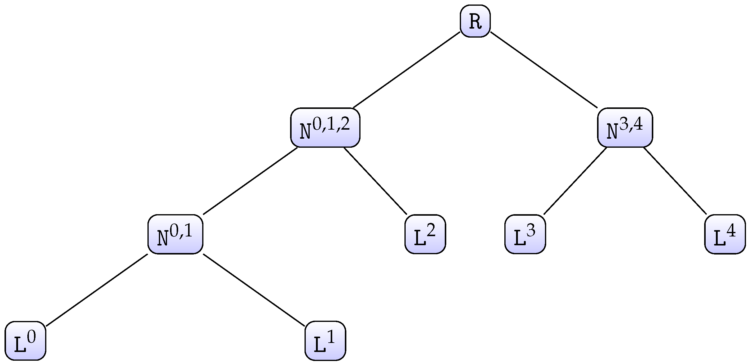
30]. To explain the complete algorithm, let us consider the case when there are five chunks as an example. We have access to five lists of chunk candidates
, each of which has a size of
. We first call
, as defined in Algorithm 2. This function will build a tree-like structure from the five given lists (see
Figure 1).
Each node is a 6-tuple of the form , where and are the children nodes, is a priority queue, and are bit vectors, and a list of chunk candidates. Additionally, this data structure supports the method , which returns the maximum number of chunk candidates that this node can generate. This method is easily defined in a recursive way: if is a leaf node, then the method will return or else, the method will return . To avoid computing this value each time this method is called, a node will internally store the value once it has been computed for the first time. Hence, the method will only return the stored value from the second call onwards. Furthermore, the function , as defined in Algorithm 3, returns the best chunk candidate (chunk candidate of which its score rank is j) from the node
In order to generate the first N best key candidates from the root node R, with , we simply run , as defined in Algorithm 4, N times. This function internally calls the function with suitable parameters each time it is required. Calling may cause this function to internally invoke to generate ordered key candidates from the inner node on the fly. Therefore, any inner node should keep track of the chunk candidates returned by when called by its parent; otherwise, the j best chunk candidates from would have to be generated each time such a call is done, which is inefficient. To keep track of the returned chunk candidates, each node updates its internal list (see lines 5 to 7 in Algorithm 3).
| Algorithm 2 creates and initialises each node of the tree-like structure. |
- 1:
functioninitialise() - 2:
if then - 3:
- 4:
return ; - 5:
else - 6:
; - 7:
; - 8:
; - 9:
; - 10:
; - 11:
; - 12:
; - 13:
- 14:
return ; - 15:
end if - 16:
end function
|
| Algorithm 3 outputs the best chunk candidate from the node . |
- 1:
functiongetCandidate() - 2:
if is a leaf then - 3:
return ; - 4:
end if - 5:
if then - 6:
; - 7:
end if - 8:
return ; - 9:
end function
|
| Algorithm 4 outputs the next highest-scoring chunk candidate from the node . |
- 1:
functionnextCandidate() - 2:
- 3:
- 4:
if and then - 5:
- 6:
- 7:
- 8:
end if - 9:
if and then - 10:
- 11:
; - 12:
- 13:
end if - 14:
return - 15:
end function
|
4.1.4. Memory Consumption
Let us suppose that the encoding of a secret key is bits in size and that we set ; therefore, . Hence, we have access to lists , , each of which has chunk candidates. Suppose we would like to generate the first N best key candidates. We first invoke (Algorithm 2). This call will create a tree-like structure with levels starting at 0.
The root node at level 0.
The inner nodes with , where is the level and is the node identification at level .
The leaf nodes at level b for .
This tree will have nodes.
Let be the number of bits consumed by chunk candidates stored in memory after calling the function nextCandidate with R as a parameter k times. A chunk candidate at level is of the form with being a real number and being bit strings. Let be the number of bits a chunk candidate at level occupies in memory.
First note that invoking causes each internal node’s list to grow, since
At creation of nodes (lines 2 to 4), is created by setting ’s internal list to and by setting ’s other components to null.
At creation of both and nodes , for and , the execution of the function getCandidate (lines 9 to 10) makes their corresponding left child (right child) store a new chunk candidate in their corresponding internal list. That is, for , the ’s internal list has a new element.
Therefore,
Suppose the best key candidate is about to be generated, then will be executed for the first time. This routine will remove the extended candidate out of R’s priority queue. If it enters the first if (lines 4 to 8), it will make the call (line 5), which may cause each node, except for the leaf nodes, of the left sub-tree to store at most a new chunk candidate in its corresponding internal list. Hence, retrieving the chunk candidate may cause at most chunk candidates per level to be stored. Likewise, if it enters the second if (lines 9 to 13), it will call the function (line 10), which may cause each node, except for the leaf nodes, of the right sub-tree to store at most a new chunk candidate in its corresponding internal list. Therefore, retrieving the chunk candidate (line 10) may cause at most chunk candidates per level , to be stored. Therefore, after generating the best key candidate, chunk candidates per level , will be stored in memory; hence, bits are consumed by chunk candidates stored in memory.
Let us assume that
key candidates have already been generated; therefore,
bits are consumed by chunk candidates in memory, with
. Let us now suppose the
best key candidate is about to be generated; then, the method
will be executed for the
time. This routine will remove the best extended candidate
out of the
R’s priority queue. It will then attempt to insert two new extended candidates into
R’s priority queue. As seen previously, retrieving the chunk candidate
may cause at most
chunk candidates per level
to be stored. Likewise, retrieving the chunk candidate
may also cause at most
chunk candidates per level
to be stored. Therefore, after generating the
best key candidate,
chunk candidates per level
, will be stored in memory; hence,
bits are consumed by chunk candidates stored in memory.
It follows that, if
N key candidates are generated, then
bits are consumed by chunk candidates stored in memory in addition to the extended candidates stored internally in the priority queue of the nodes
R and
Therefore, this algorithm may consume a large amount of memory if it is used to generate a large number of key candidates, which may be problematic.
4.4. Complete Algorithm
When the number of chunks is greater than 2, the algorithm applies a recursive decomposition of the problem (similar to OKEA). Whenever a new chunk candidate is inserted into the candidate set, its value is obtained by applying the enumeration algorithm to the lower level. We explain an example to give an idea of the general algorithm. Let us suppose the encoding of the secret key is divided into 4 chunks; then, we have access to 4 lists of chunk candidates, each of which is of size with
To generate key candidates, we need to generate the two lists of chunk candidates for the lower level
and
on the fly as far as required. For this, we maintain a set of next potential candidates, for each dimension,
and
, so that each next chunk candidate obtained from
(or
) is stored in the list
(or
). Because the enumeration is performed by layers, the sizes of the data structures
and
are bounded by
. However, this is not the case for the lists
and
, which grow as the number of candidates enumerated grows, hence becoming problematic as seen in
Section 4.1.4.
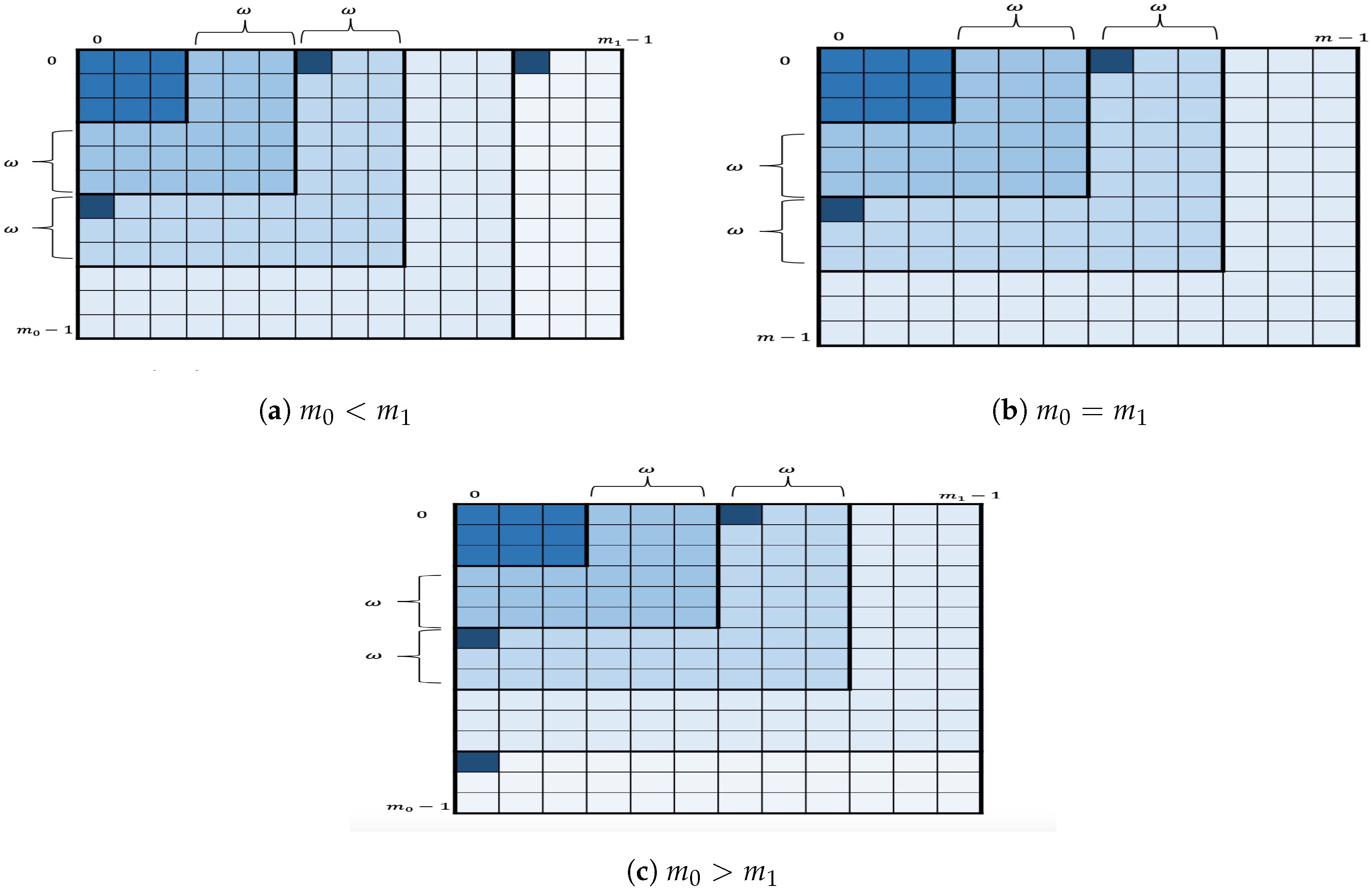
To handle this, each
is partitioned into squares of size
. The algorithm still enumerates the key candidates in
first, then in
, and so on, but in each
, the enumeration will be square-by-square.
Figure 3 depicts the geometric representation of the key enumeration within
where a square (strong shade of blue) within a layer represents the square being processed by the enumeration algorithm. More specifically, for given nonnegative integers
I and
let us define
as
Let us set
; hence,
for
. The remaining layers, if any, are also partitioned in a similar way.
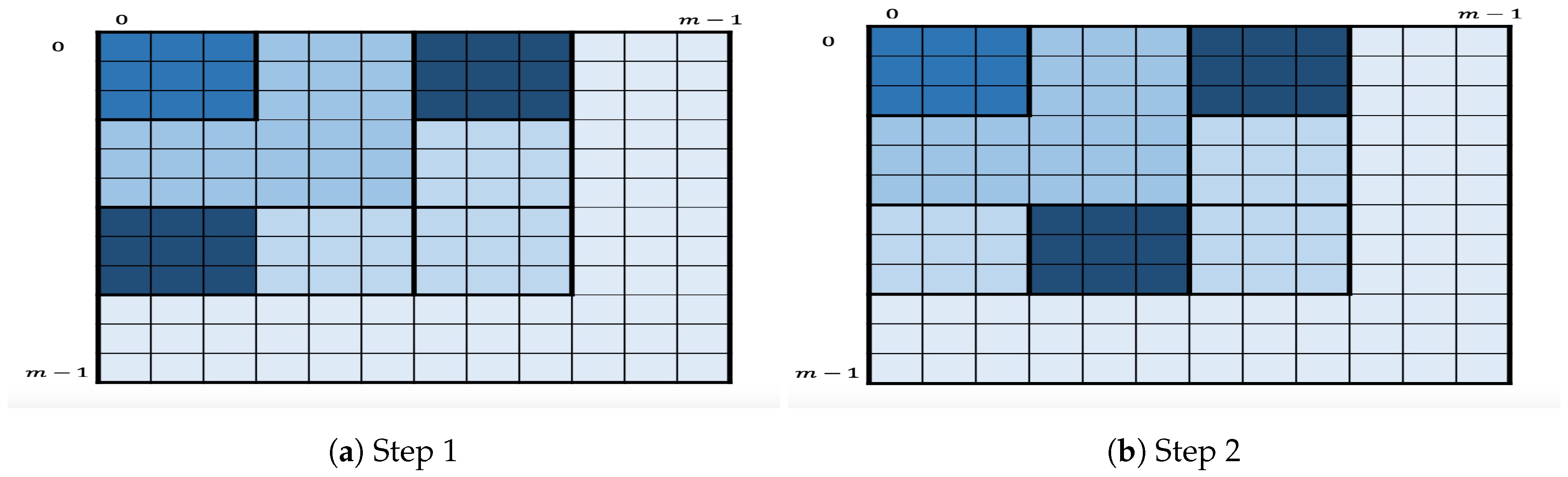
The in-layer algorithm then proceeds as follows. For each the in-layer algorithm first enumerates the candidates in the two corner squares by applying OKEA on S. At some point, one of the two squares is completely enumerated. Assume this is . At this point, the only square that contains the next key candidates after is the successor . Therefore, when one of the squares is completely enumerated, its successor is inserted in S, as long as S does not contain a square in the same row or column. For the remaining layers, if any, the in-layer algorithm first enumerates the candidates in the square (or ) by applying OKEA on it. Once the square is completely enumerated, its successor is inserted in S, and so on. This in-layer partition into squares reduces the space complexity, since instead of storing the full list of chunk candidates of the lower levels, only the relevant chunk candidates are stored for enumerating the two current squares.
Because this in-layer algorithm enumerates at most two squares at any time in a layer, the tree-like structure is no longer a binary tree. A node is now extended to an 8-tuple of the form , where and for are the children nodes used to enumerate at most two squares in a particular layer, is a priority queue, and are bit vectors, and is a list of chunk candidates. Hence, the function that initialises the tree-like structure is adjusted to create the two additional children for a given node (see Algorithm 5).
| Algorithm 5 creates and initialises each node of the tree-like structure. |
- 1:
functioninitialise() - 2:
if then - 3:
- 4:
return ; - 5:
else - 6:
; - 7:
; - 8:
; - 9:
; - 10:
; - 11:
; - 12:
; - 13:
; - 14:
; ; - 15:
; - 16:
return ; - 17:
end if - 18:
end function
|
| Algorithm 6 outputs the chunk candidate from the node . |
- 1:
functiongetCandidate() - 2:
if is a leaf then - 3:
return ; - 4:
end if - 5:
if then - 6:
; - 7:
else - 8:
if then - 9:
; - 10:
end if - 11:
end if - 12:
; - 13:
if then - 14:
; - 15:
end if - 16:
return ; - 17:
end function
|
| Algorithm 7 outputs the next chunk candidate from the node . |
- 1:
functionnextCandidate() - 2:
- 3:
- 4:
- 5:
if is completely enumerated then - 6:
; - 7:
; - 8:
if or ( and ) or ( and) then - 9:
if then - 10:
- 11:
- 12:
- 13:
- 14:
end if - 15:
if then - 16:
- 17:
- 18:
- 19:
- 20:
end if - 21:
else - 22:
if no candidates in same row/column as then - 23:
; - 24:
- 25:
- 26:
end if - 27:
end if - 28:
else - 29:
if and is set to 0 then - 30:
- 31:
- 32:
- 33:
end if - 34:
if and is set to 0 then - 35:
if then - 36:
- 37:
else - 38:
- 39:
end if - 40:
- 41:
- 42:
end if - 43:
end if - 44:
return ; - 45:
end function
|
Moreover, the function is also adjusted so that each node’s internal list has at most chunk candidates at any stage of the algorithm (see Algorithm 6). This function internally makes the call to if . The call to causes to restart its enumeration, i.e., after has been invoked, calling will return the first chunk candidate from . Also, the function returns the highest-scoring extended candidate from the square . Note this function is called to get the highest-scoring extended candidate from the successor of . At this point, the content of the internal list of is cleared if . Otherwise, the content of the internal list of is cleared, if . Finally, Algorithm 7 precisely describes the manner in which this enumeration works.
4.4.1. Parallelization
The original authors of the research paper [
13] suggest having OKEA run in parallel per square within a layer, but this has a negative effect on the algorithm’s near-optimality property and even on its overall performance since there are squares within a layer that are strongly dependent on others, i.e., for the algorithm to enumerate the successor square, say,
within a layer, it requires having information that is obtained during the enumeration of
. Hence, this strategy may incur extra computation and is also difficult to implement.
4.4.2. Variant
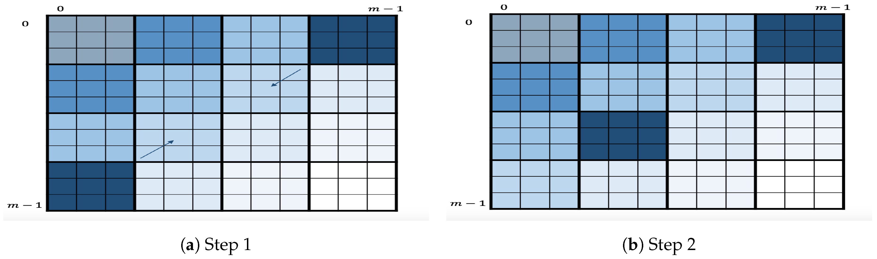
As a variant of this algorithm, we propose to slightly change the definition of layer. Here, a layer consists of all the squares within a secondary diagonal, as shown in
Figure 4. The variant will follow the same process as the original algorithm, i.e., enumeration layer by layer starting at the first secondary diagonal. Within each layer, it will first enumerate the two square corners
by applying OKEA on it. Once one of two squares is enumerated, let us say
, its successor
will be inserted in
S as long as such insertion is possible. The algorithm will continue the enumeration by applying OKEA on the updated
S and so on. This algorithm is motivated by the intuition that enumerating secondary diagonals may improve the quality of order of output key candidates, i.e., it may be closer to optimal. This variant, however, may have a potential disadvantage in the multidimensional case because it strongly depends on having all the previously enumerated chunk candidates of both dimension
x and
y stored. To illustrate this, let us suppose that this square
is to be inserted. Then, the algorithm needs to insert its highest-scoring extended candidate,
, into the queue. Hence, the algorithm needs to somehow have both
and
readily accessible when needed. This implies the need to store them when they are being enumerated (in previous layers). Comparatively, the original algorithm only requires having the
previously generated chunk candidates of both dimension
x and
y stored, which is advantageous in terms of memory consumption.
4.5. A Simple Stack-Based, Depth-First Key Enumeration Algorithm
We next present a memory-efficient, nonoptimal key enumeration algorithm that generates key candidates of which their total scores are within a given interval
that is based on the algorithm introduced by Martin et al. in the research paper [
16]. We note that the original algorithm is fairly efficient while generating a new key candidate; however, its overall performance may be negatively affected by its use of memory, since it was originally designed to store each new generated key candidate, each of which is tested only once the algorithm has completed the enumeration. Our variant, however, makes use of a stack (last-in-first-out queue) during the enumeration process. This helps in maintaining the state of the algorithm. Each newly generated key candidate may be tested immediately, and there is no need for candidates to be stored for future processing.
Our variant basically performs a depth-first search in an undirected graph G originated from the lists of chunk candidates . This graph G has vertices, each of which represents a chunk candidate. Each vertex is connected to the vertices . At any vertex , the algorithm will check if plus an accumulated score is within the given interval . If so, it will select the chunk candidate for the chunk i and travel forward to the vertex , or else, it will continue exploring and attempt to travel to the vertex . Otherwise, it will travel backwards to a vertex from the previous chunk , when there is no suitable chunk candidate for the current chunk i.
As can be noted, this variant uses a simple backtracking strategy. In order to speed up the pruning process, we will make use of two precomputed tables
. The entry
holds the global minimum (maximum) value that can be reached from chunk
i to chunk
. In other words,
with
Additionally, note that when each list of chunk candidates
, is in decreasing order based on the score component of its chunk candidates, we can compute the entry
by computing
and
Therefore, the basic variant is sped up by computing maxS (minS), which is the maximum(minimum) score that can be obtained from the current chunk candidate, and then by checking if the intersection of the intervals and is not empty.
4.5.1. Setup
We now introduce a couple of tools that we will use to describe the algorithm, using the following notations.
will denote a stack. This data structure supports two basic methods [
30]. Firstly, the method
removes the element at the top of this stack and returns that element as the value of this function. Secondly, the method
pushes
e onto the top of this stack. This stack
S will store 4-tuples of the form
, where
is the accumulated score at any stage of the algorithm,
i and
j are the indices for the chunk candidate
, and
is an array of positive integers holding the indices of the selected chunk candidates, i.e., the chunk candidate
is assigned to chunk
k and for each k,
.
4.5.2. Complete Algorithm
Firstly, at the initialisation stage, the 4-tuple will be inserted into the stack . The main loop of this algorithm will call the function , defined in Algorithm 8, as long as the stack is not empty. Specifically the main loop will call this function to obtain a key candidate of which its score is in the range . Algorithm 8 will then attempt to find such a candidate, and once it has found such a candidate, it will return the candidate to the main loop (at this point, may not be empty). The main loop will get the key candidate, process or test it, and continue calling the function as long as S is not empty. Because of the use of the stack S, the state of Algorithm 8 will not be lost; therefore, each time the main loop calls it, it will return a new key candidate of which its score lies in the interval . The main loop will terminate once all possible key candidates of which their scores are within the interval have already been generated, which will happen once the stack is empty.
| Algorithm 8 outputs a key candidate in the interval . |
- 1:
functionNextCandidate() - 2:
while S is not empty do - 3:
- 4:
if then - 5:
; - 6:
end if - 7:
; - 8:
- 9:
- 10:
if and then - 11:
if then - 12:
if then - 13:
if then - 14:
; - 15:
- 16:
- 17:
end if - 18:
else - 19:
; - 20:
end if - 21:
end if - 22:
end if - 23:
end while - 24:
return ; - 25:
end function
|
4.5.3. Memory Consumption
We claim that, at any stage of the algorithm, there are at most 4-tuples stored in the stack S. Indeed, after the stack is initialised, it only contains the 4-tuple . Note that, during the execution of a while iteration, a 4-tuple is removed out of the stack and two new 4-tuples might be inserted. Hence, after s while iterations have been completed, there will be 4-tuples, where , for .
Suppose now that the algorithm is about to execute the while iteration during which the first valid key candidate will be returned. Therefore, During the execution of the while iteration, a 4-tuple will be removed and only a new 4-tuple will be considered for insertion in the stack. Therefore, we have that , since . Applying a similar reasoning, we have for .
4.5.4. Parallelization
One of the most interesting features of the previous algorithm is that it is parallelizable. The original authors suggested as a parallelization method to run instances of the algorithm over different disjoint intervals [
16]. Although this method is effective and has a potential advantage as the different instances will produce nonoverlapping lists of key candidates with the instance searching over the first interval producing the most-likely key candidates, it is not efficient since each instance will inevitably repeat a lot of the work done by the other instances. Here, we propose another parallelization method that partitions the search space to avoid the repetition of work.
Suppose that we want to have t parallel, independent tasks to search over a given interval in parallel. Let be the list of chunk candidates for chunk i, .
We first assume that , where is the size of . In order to construct these tasks, we partition into t disjoint, roughly equal-sized sublists . We set each task to perform its enumeration over the given interval but only consider the lists of chunk candidates .
Note that the previous startegy can be easily generalised for . Indeed, first, find the smallest integer l, with , such that . We then construct the list of chunk candidates as follows. For each -tuple , with , the chunk candidate is constructed by calculating and by setting , and then, is added to . We then partition into t disjoint, roughly equal-sized sublists and finally set each task to perform its enumeration over the given interval but only consider the lists of chunk candidates . Note that the workload assigned to each enumerating task is a consequence of the selected method for partitioning the list .
Additionally, both parallelization methods can be combined by partitioning the given interval into disjoint subintervals and by searching each such subinterval with tasks, hence amounting to enumerating tasks.
4.6. Threshold Algorithm
Algorithm 8 shares some similarities with the algorithm Threshold introduced in the research paper [
14], since Threshold also makes use of an array (
partialSum) similar to the array
minArray to speed up the pruning process. However, Threshold works with nonnegative integer values (weights) rather than scores. Threshold restricts the scores to weights such that the smallest weight is the likeliest score by making use of a function that converts scores into weights [
14].
Assuming the scores have already been converted to weights, Threshold first sorts each list of chunk candidates in ascending order based on the score/weight component of its chunk candidates. It then computes the entries of partialSum by first setting and then by computing
Threshold then enumerates all the key candidates of which their accumulated total weight lies in a range of the form , where is a parameter. To do so, it performs a similar process to Algorithm 8 by using its precomputed table (partialSum) to avoid useless paths, hence improving the pruning process. This enumeration process performed by Threshold is described in Algorithm 9.
According to its designers, this algorithm may perform a nonoptimal enumeration to a depth of
if some adjustments are made in the data structure
L used to store the key candidates. However, its primary drawback is that it must always start enumerating from the most likely key. Consequently, whilst the simplicity and relatively strong time complexity of Threshold is desirable, in a parallelized environment, it can only serve as the first enumeration algorithm (or can only be used in the first search task). Threshold, therefore, was not implemented and, hence, is not included in the comparison made in
Section 5.
| Algorithm 9 enumerates all key candidate in the interval . |
- 1:
functionthreshold() - 2:
for do - 3:
- 4:
if then - 5:
- 6:
else - 7:
if then - 8:
- 9:
- 10:
- 11:
else - 12:
- 13:
- 14:
end if - 15:
end if - 16:
end for - 17:
return L; - 18:
end function
|
4.7. A Weight-Based Key Enumeration Algorithm
In this subsection, we will describe a nonoptimal enumeration algorithm based on the algorithm introduced in the research paper [
12]. This algorithm differs from the original algorithm in the manner in which this algorithm builds a precomputed table (
iRange) and uses it during execution to construct key candidates of which their total accumulated score is equal to a certain accumulated score. This algorithm shares similarities with the stack-based, depth-first key enumeration algorithm described in
Section 4.5 because both algorithms essentially perform a depth-first search in the undirected graph
G. However, this algorithm controls pruning by the accumulated total score that a key candidate must reach to be accepted. To achieve this, the scores are restricted to positive integer values (weights), which may be derived from a correlation value in a side-channel analysis attack.
This algorithm starts off by generating all key candidates with the largest possible accumulated total weight
and then proceeds to generate all key candidates of which their accumulated total weight are equal to the second largest possible accumulated total weight
, and so forth, until it generates all key candidates with the minimum possible accumulated total weight
. To find a key candidate with a weight equal to a certain accumulated weight, this algorithm makes use of a simple backtracking strategy, which is efficient because impossible paths can be pruned early. The pruning is controlled by the accumulated weight that must be reached for the solution to be accepted. To achieve a fast decision process during backtracking, this algorithm precomputes tables for minimal and maximal accumulated total weights that can be reached by completing a path to the right, like the tables
minArray and
maxArray introduced in
Section 4.5. Additionally, this algorithm precomputes an additional table,
iRange.
Given and , the entry points to a list of integers , where each entry represents a distinct index of the list , i.e., for . The algorithm uses these indices to construct a chunk candidate with an accumulated score w from chunk i to chunk .
In order to compute this table, we use the observation that for a given entry of , the list , with , must be defined and be nonempty. So we first set the entry to and then proceed to compute the entries for and . Algorithm 10 describes precisely how this table is precomputed.
| Algorithm 10 precomputes the table iRange. |
- 1:
functionPrecomputeIRange( ) - 2:
; - 3:
for to 0 do - 4:
for to do - 5:
- 6:
for to do - 7:
; - 8:
if then - 9:
; - 10:
end if - 11:
end for - 12:
if then - 13:
; - 14:
end if - 15:
end for - 16:
end for - 17:
return - 18:
end function
|
4.7.1. Complete Algorithm
Algorithm 11 describes the backtracking strategy more precisely, making use of the precomputed tables for pruning impossible paths. The integer array TWeights contains accumulated weights in a selected order, where an entry must satisfy that the list is non-empty, i.e., . This helps in constructing a key candidate with an accumulated score w from chunk 0 to chunk . In particular, TWeights may be set to , i.e., the array containing all possible accumulated scores that can be reached from chunk 0 to chunk .
Furthermore, the order in which the elements in the array TWeights are arranged is important. For this array , for example, the algorithm will first enumerate all key candidates with accumulated weight and then all those with accumulated weight and so on. This guarantees a certain quality, since good key candidates will be enumerated earlier than worse ones. However, key candidates with the same accumulated weight will be generated in no particular order, so a lack of precision in converting scores to weights will lead to some decrease of quality.
| Algorithm 11 enumerates key candidates for given weights. |
- 1:
functionKeyEnumeration(TWeights, iRange) - 2:
for do - 3:
; - 4:
; 2-tuple - 5:
- 6:
while do - 7:
while do - 8:
- 9:
- 10:
- 11:
end while - 12:
- 13:
- 14:
while and do - 15:
- 16:
if then - 17:
- 18:
end if - 19:
end while - 20:
if then - 21:
- 22:
end if - 23:
end while - 24:
end for - 25:
end function
|
Algorithm 11 makes use of the table with entries, each of which is a 2-tuple of the form with and integers. For a given tuple , the component is an index of some list , with , while is the corresponding value, i.e., . The value of allows the algorithm to control if the list has been traveled completely or not, while the second component allows the algorithm to retrieve the chunk candidate of index of . This is done to avoid recalculating each time it is required during the execution of the algorithm.
We will now analyse Algorithm 11. Suppose that ; hence, . The algorithm will then set to , with being the integer from the entry of index 0 of , and then set to w (lines 3 to 5). We claim that the main while loop (lines 6 to 23) at each iteration will compute for such that the key candidate constructed at line 12 will have an accumulated score w.
Let us set . We know that the list is non-empty; hence, for any entry in the list , the list is non-empty, where
Likewise, for any entry in the list , the list is non-empty, where
Hence, for , we have that, for any given entry in the list , the list is non-empty, where
Note that, when , the list is non-empty and .
Given are already set for some ; the first inner while loop (lines 7 to 11) will set , where holds the entry of index 0 of , for . Therefore, once the while loop ends, and . Hence, the key candidate constructed from the second components will have an accumulated score w. In particular, the first time is set, and so, the first inner while loop will calculate .
Since there may be more than one key candidate with an accumulated score w, the second inner while loop (lines 14 to 19) will backtrack to a chunk , from which a new key candidate with accumulated score w can be constructed. This is done by simply moving backwards (line 15) and updating to until there is an i, , such that .
If there is such an i, then the instruction at line 21 will update to . This means that the updated value for the second component of will be a valid index in , so will be the new chunk candidate for chunk i. Then, the first inner while loop (lines 7 to 11) will again execute and compute the indices for the remaining chunk candidates in the lists such that the resulting key candidate will have the accumulated score w.
Otherwise, if , then the main while loop (lines 6 to 23) will end and w will be set to a new value from TWeights, since all key candidates with an accumulated score w have just been enumerated.
4.7.2. Parallelization
Suppose we would like to have t tasks executed in parallel to enumerate key candidates of which the accumulated total weights are equal to those in the array . We can split the array into t disjoint sub-arrays and then set each task to run Algorithm 11 through the sub-array . As an example of a partition algorithm to distribute the workload among the tasks, we set the sub-array to contain elements with indices congruent to i mod t from . Additionally, note that, if we have access to the number of candidates to be enumerated for each score in the array beforehand, we may design a partition algorithm for distributing the workload among the tasks almost evenly.
4.7.3. Run Times
We assume each list of chunk candidates
, is in decreasing order based on the score component of its chunk candidates. Regarding the run time for computing the tables
maxArray and
minArray, note that each entry of the table
can be computed as explained in
Section 4.5. Therefore, the run time of such an algorithm is
.
Regarding the run time for computing iRange, we will analyse Algorithm 10. This algorithm is composed of three For blocks. For each i, , the For loop from line 4 to line 15 will be executed times, where . For each iteration, the innermost For block (lines 6 to 11) will execute simple instructions times. Therefore, once the innermost block has finished, its run time will be , where and are constants. Then, the if block (lines 12 to 14) will be attempted and its run time will be , where is another constant. Therefore, the run time for an iteration of the For loop (lines 4 to 15) will be . Therefore, the run time of Algorithm 10 is . More specifically,
As noted, this run time depends heavily on . Now, the size of the range relies on the scaling technique used to get a positive integer from a real number. The more accurate the scaling technique is, the more different integer scores there will be. Hence, if we use an accurate scaling technique, we will probably get larger .
We will analyse the run time for Algorithm 11 to generate all key candidates of which their total accumulated weight is w. Let us assume there are key candidates of which their total accumulated score is equal to w.
First, the run time for instructions at lines 3 to 5 is constant. Therefore, we will only focus on the while loop (lines 6 to 23). In any iteration, the first inner while loop (lines 7 to 11) will execute and compute the indices for the remaining chunk candidates in the lists , with i starting at any number in , such that the resulting key candidate will have the accumulated score w. Therefore, its run time is at most , where C is a constant, i.e., it is . The instruction at line 12 will combine all chunks from 0 to , and hence, its run time is also . The next instruction will test c, and its run time will depend on the scenario in which the algorithm is being run. Let us assume its run time is , where T is a function.
Regarding the second inner while loop (lines 14 to 19), this loop will backtrack to a chunk i with , from which a new key candidate with accumulated score w can be constructed. This is done by simply moving backwards while computing some simple operations. Therefore, the run time for the second inner while loop is at most , where D is a constant, i.e., it is . Therefore, the run time for generating all key candidates of which the total accumulated score is w will be .
4.7.4. Memory Consumption
Besides the precomputed tables, it is easy to see that Algorithm 11 makes use of negligible memory while enumerating key candidates. Indeed, testing key candidates is done on the fly to avoid storing them during enumeration. However, the table iRange may have many entries.
Let be the number of entries of the table iRange. Line 2 of Algorithm 10 will create the entry that points to the list . Hence, after the instruction at line 2 has been executed, . Let us consider the For block from line 4 to line 15. For each i, , let be the set of different values w in the range such that is non-empty. After the iteration for i has been executed, the table iRange will have new entries, each of which will point to a non-empty list, with Therefore, after Algorithm 10 has completed its execution.
Note that may increase if the range is large. The size of this interval relies on the scaling technique used to get a positive integer from a real number. The more accurate the scaling technique is, the more different integer scores there will be. Hence, if we use an accurate scaling technique, we will probably get larger , making it likely for to increase. Therefore, the table iRange may have many entries.
Regarding the number of bits used in memory to store the table
iRange, let us suppose that an integer is stored in
bits and that a pointer is stored in
bits. Once Algorithm 10 has completed its execution, we know that
will point to the list
, with
and
Moreover, by definition, we know that the list
will be the list
, while any other list
,
and
, will have
entries, with
. Therefore, the number of bits
iRange occupies in memory after Algorithm 11 has completed its execution is
Since
, we have
4.8. A Key Enumeration Algorithm using Histograms
In this subsection, we will describe a nonoptimal key enumeration algorithm introduced in the research paper [
17].
4.8.1. Setup
We now introduce a couple of tools that we will use to describe the sub-algorithms used in the algorithm of the research paper [
17], using the following notations:
H will denote a histogram,
will denote a number of bins,
b will denote a bin, and
x will denote a bin index.
Linear Histograms
The function creates a standard histogram from the list of chunk candidates with linearly spaced bins.
Given a list of chunk candidates , the function createHist will first calculate both the minimum score and maximum score among all the chunk candidates in . It will then partition the interval into subintervals , where It then will proceed to build the list of size . The entry of will point to a list that contains all chunk candidates from such that their scores lie in . The returned standard histogram is therefore stored as the list of which its entries will point to lists of chunk candidates. For a given bin index x, outputs the list of chunk candidates contained in the bin of index x of Therefore, is the number of chunk candidates in the bin of index x of . The run time for is .
Convolution
This is the usual convolution algorithm which computes
from two histograms
and
of sizes
and
, respectively, where
The computation of
is done efficiently by using Fast Fourier Transformation (FFT) for polynomial multiplication. Indeed, the array
is seen as the coefficient representation of
for
In order to get
, we multiply the two polynomials of degree-bound
in time
, with both the input and output representations in coefficient form [
30]. The convoluted histogram
is therefore stored as a list of integers.
Getting the Size of a Histogram
The method size() returns the number of bins of a histogram. This method simply returns , where L is the underlying list used to represent the histogram.
Getting Chunk Candidates from a Bin
Given a standard histogram and an index , the method outputs the list of all chunk candidates contained in the bin of index x of , i.e., this method simply returns the list
4.8.2. Complete Algorithm
This key enumeration algorithm uses histograms to represent scores, and the first step of the key enumeration is a convolution of histograms modelling the distribution of the lists of scores. This step is detailed in Algorithm 12.
| Algorithm 12 computes standard and convoluted histograms. |
- 1:
functioncreateHistograms() - 2:
; - 3:
; - 4:
; - 5:
for to do - 6:
; - 7:
; - 8:
end for - 9:
return ; - 10:
end function
|
Based on this first step, this key enumeration algorithm allows enumerating key candidates that are ranked between two bounds and . In order to enumerate all keys ranked between the bounds and , the corresponding indices of bins of have to be computed, as described in Algorithm 13. It simply sums the number of key candidates contained in the bins starting from the bin containing the highest scoring key candidates until we exceed and and returns the corresponding indices and
| Algorithm 13 computes the indices’ bounds. |
- 1:
functioncomputeBounds() - 2:
; - 3:
; - 4:
while do - 5:
; - 6:
; - 7:
end while - 8:
; - 9:
while do - 10:
; - 11:
; - 12:
end while - 13:
; - 14:
return ; - 15:
end function
|
Given the list of histograms of scores H and the indices of bins of between which we want to enumerate, the enumeration simply consists of performing a backtracking over all the bins between and . More precisely, during this phase, we recover the bins of the initial histograms (i.e., before convolution) that were used to build a bin of the convoluted histogram . For a given bin b with index x of , we have to run through all the non-empty bins of indices of such that . Each will then contain at least one and at most chunk candidates of the list that we must enumerate. This leads to storing a table of entries, each of which points to a list of chunk candidates. The list pointed to by the entry holds at least one and at most chunk candidates contained in the bin of the histogram Any combination of these lists, i.e., picking an entry from each list, results in a key candidate.
Algorithm 14 describes more precisely this bin decomposition process. This algorithm simply follows a recursive decomposition. That is, in order to enumerate all the key candidates within a bin b of index x of , it first finds two non-empty bins of indices and of and , respectively. All the chunk candidates in the bin of index of will be added to the key factorisation, i.e., the entry will point to the list of chunk candidates returned by . It then continues the recursion with the bin of index of by finding two non-empty bins of indices and of and , respectively, and by adding all the chunk candidates in the bin of index of to the key factorisation, i.e., will now point to the list of chunk candidates returned by and so forth. Eventually, each time a factorisation is completed, Algorithm 14 calls the function processKF, which takes as input the table kf. The function processKF, as defined in Algorithm 15, will compute the key candidates from kf. This algorithm basically generates all the possible combinations from the lists . Note that this algorithm may be seen as a particular case of Algorithm 11. Finally, the main loop of this key enumeration algorithm simply calls Algorithm 14 for all the bins of , which are between the enumeration bounds .
| Algorithm 14 performs bin decomposition. |
- 1:
functionDecomposeBin() - 2:
if then - 3:
; - 4:
while and do - 5:
if and then - 6:
; - 7:
; - 8:
; - 9:
end if - 10:
; - 11:
end while - 12:
else - 13:
; - 14:
while and do - 15:
if and then - 16:
; - 17:
; - 18:
end if - 19:
; - 20:
end while - 21:
end if - 22:
end function
|
4.8.3. Parallelization
Suppose we would like to have t tasks executing in parallel to enumerate key candidates that are ranked between two bounds and in parallel. We can then calculate the indices and and then create the array . We then partition the array into t disjoint sub-arrays and finally set each task to call the function decomposeBin for all the bins of with indices in .
As has been noted previously, the algorithm employed to partition the array directly allows efficient parallel key enumeration, where the amount of computation performed by each task may be well balanced. An example of a partition algorithm that could almost evenly distribute the workload among the tasks is as follows:
Set i to 0.
If is non-empty, pick an index x in such that is the maximum number or else return
Remove x from the array , and add it to the array .
Update i to , and go back to Step 2.
| Algorithm 15 processes table kf. |
- 1:
functionproccessKF() - 2:
; - 3:
; - 4:
while do - 5:
while do - 6:
; - 7:
; - 8:
end while - 9:
; - 10:
; - 11:
while and do - 12:
; - 13:
end while - 14:
if then - 15:
- 16:
end if - 17:
end while - 18:
end function
|
4.8.4. Memory Consumption
Besides the precomputed histograms, which are stored as arrays in memory, it is easy to see that this algorithm makes use of negligible memory (only table kf) while enumerating key candidates. Additionally, it is important to note that each time the function is called, it will need to generate all key candidates obtained by picking chunk candidates from the lists pointed to by the entries of and to process all of them immediately, since the table may have changed. This implies that, if the processing of key candidates is left to be done after the complete enumeration has finished, each version of the table would need to be stored, which, again, might be problematic in terms of memory consumption.
Regarding how many bits in memory the precomputed histograms consumes, we will analyse Algorithm 12. First, note, for a given list of chunk candidates
and
, the function
will return the standard histogram
. This standard histogram will be stored as the list
of size
. An entry
x of
will point to a list of chunk candidates. The total number of chunk candidates held by all the lists pointed to by the entries of
is
. Therefore, the number of bits to store the list
is
, where
is the number of bits to store a pointer and
is the number of bits to store a chunk candidate
. The total number of bits to store all lists
is
Concerning the convoluted histograms, let us first look at
. We know that
is stored as a list of integers and that these entries can be seen as the coefficients of the resulting polynomial from multiplying the polynomial
by
. Therefore, the list of integers used to store
has
entries. Following a similar reasoning to the previous one, we can conclude that the list of integers used to store
has
entries. Therefore, for a given
, the list of integers used to store
has
entries. The total number of entries of all the convoluted histograms
is
As expected, the total number of entries strongly depends on the values
and
. If an integer is stored in
bits, then the number of bits for storing all the convoluted histograms is
4.8.5. Equivalence with the Path-Counting Approach
The stack-based key enumeration algorithm and the score-based key enumeration algorithm can be also used for rank computation (instead of enumerating each path, the rank version counts each path). Similarly, the histogram algorithm can also be used for rank computation by simply summing the size of the corresponding bins in
. These two approaches were believed to be distinct from each other. However, Martin et al. in the research paper [
31] showed that both approaches are mathematically equivalent, i.e., they both compute the exact same rank when choosing their discretisation parameter correspondingly. Particularly, the authors showed that the binning process in the histogram algorithm is equivalent to the “map to weight” float-to-integer conversion used prior to their path counting algorithm (Forest) by choosing the algorithms’ discretisation parameter carefully. Additionally, in this paper, a performance comparison between their enumeration versions was carried out. The practical experiments indicated that Histogram performs best for low discretisation and that Forest wins for higher parameters.
4.8.6. Variant
A recent paper by Grosso [
26] introduced a variant of the previous algorithm. Basically, the author of [
26] makes a small adaptation of Algorithm 14 to take into account the tree-like structure used by their rank estimation algorithm. Also, the author claims this variant has an advantage over the previous one when the memory needed to store histograms is too large.
4.9. A Quantum Key Search Algorithm
In this subsection, we will describe a quantum key enumeration algorithm introduced in the research paper [
29] for the sake of completeness. This algorithm is constructed from a nonoptimal key enumeration algorithm, which uses the key rank algorithm given by Martin et al. in the research paper [
16] to return a single key candidate (the
) with a weight in a particular range. We will first describe the key rank algorithm. This algorithm restricts the scores to positive integer values (weights) such that the smallest weight is the likeliest score by making use of a function that converts scores into weights [
16].
Assuming the scores have already been converted to weights, the rank algorithm first constructs a matrix with size of for a given range as follows. For and , the entry contains the number of chunk candidates such that their total score plus w lies in the given range. Therefore, is given by the number of chunk candidates , such that .
On the other hand, for and , the entry contains the number of chunk candidates that can be constructed from the chunk i to the chunk such that their total score plus w lies in the given range. Therefore, may be calculated as follows. For if
Algorithm 16 describes precisely the manner in which the matrix is computed. Once matrix is computed, the rank algorithm will calculate the number of key candidates in the given range by simply returning . Note that , by construction, contains the number of chunk candidates, with initial weight 0, that can be constructed from the chunk 0 to the chunk such that their total weight lies in the given range. Algorithm 17 describes the rank algorithm.
| Algorithm 16 creates the matrix . |
- 1:
functioninitialise() - 2:
; - 3:
; - 4:
for do - 5:
for do - 6:
if then - 7:
; - 8:
end if - 9:
end for - 10:
end for - 11:
for do - 12:
for do - 13:
for do - 14:
if then - 15:
; - 16:
end if - 17:
end for - 18:
end for - 19:
end for - 20:
return ; - 21:
end function
|
| Algorithm 17 returns the number of key candidates in a given range. |
- 1:
functionrank() - 2:
; - 3:
return ; - 4:
end function
|
With the help of Algorithm 17, an algorithm for requesting particular key candidates is introduced, which is described in Algorithm 18. It returns the key candidate with weight between and . Note that the correctness of the function getKey follows from the correctness of and that the algorithm is deterministic, i.e., given the same r, it will return the same key candidate k. Also, note that the key candidate does not have to be the most likely key candidate in the given range.
Equipped with the
getkey algorithm, the authors of [
29] introduced a nonoptimal key enumeration algorithm to enumerate and test all key candidates in the given range. This algorithm works by calling the function
getKey to obtain a key candidate in the given range until there are no more key candidates in the given range. Also, for each obtained key candidate
k, it is tested by using a testing function
returning either 1 or 0. Algorithm 19 precisely describes how this nonoptimal key enumeration algorithm works.
| Algorithm 18 returns the key candidate with weight between and |
- 1:
functiongetKey() - 2:
if then - 3:
return ⊥; - 4:
end if end if - 5:
; - 6:
; - 7:
for do - 8:
for do - 9:
if then - 10:
; - 11:
; - 12:
break j; - 13:
end if - 14:
; - 15:
end for - 16:
end for - 17:
; - 18:
for do - 19:
; - 20:
if then - 21:
; - 22:
break j; - 23:
end if - 24:
; - 25:
end for - 26:
return ; - 27:
end function
|
Combining together the function
keySearch with techniques for searching over partitions independently, the authors of the research paper [
29] introduced a key search algorithm, described in Algorithm 20. The function
KS works by partitioning the search space into sections of which the size follows a geometrically increasing sequence using a size parameter
. This parameter is chosen such that the number of loop iterations is balanced with the number of keys verified per block.
| Algorithm 19 enumerates and tests key candidates with weight between and |
- 1:
functionkeySearch() - 2:
; - 3:
; - 4:
while do - 5:
; - 6:
if then - 7:
break; - 8:
end if - 9:
if then - 10:
break; - 11:
end if - 12:
; - 13:
end while - 14:
return ; - 15:
end function
|
| Algorithm 20 searches key candidates in a range with a size of e approximately. |
- 1:
functionKS() - 2:
; - 3:
; - 4:
; - 5:
Choose such that is approx e; - 6:
while do - 7:
; - 8:
if then - 9:
return ; - 10:
end if - 11:
; - 12:
; - 13:
Choose such that is approx ; - 14:
end while - 15:
return ⊥; - 16:
end function
|
Having introduced the function
KS, the authors of the research paper [
29] transformed it into a quantum key search algorithm that heavily relies on Grover’s algorithm [
32]. This is a quantum algorithm to solve the following problem: Given a black box function which returns 1 on a single input
x and 0 on all other inputs, find
x. Note that, if there are
N possible inputs to the black box function, the classical algorithm uses
queries to the black box function since the correct input might be the very last input tested. However, in a quantum setting, a version of Grover’s algorithm solves the problem using
queries, with certainty [
32,
33]. Algorithm 21 describes the quantum search algorithm, which achieves a quadratic speedup over the classical key search (Algorithm 20) [
29]. However, it would require significant quantum memory and a deep quantum circuit, making its practical application in the near future rather unlikely.
| Algorithm 21 performs a quantum search of key candidates in a range with a size of e approximately. |
- 1:
functionQKS() - 2:
; - 3:
; - 4:
; - 5:
Choose such that is approx e; - 6:
while do - 7:
; - 8:
; - 9:
Call Grover using for one or zero marked elements in range ; - 10:
if marked element t found then - 11:
return ; - 12:
end if - 13:
; - 14:
; - 15:
Choose such that is approx ; - 16:
end while - 17:
return ⊥; - 18:
end function
|


