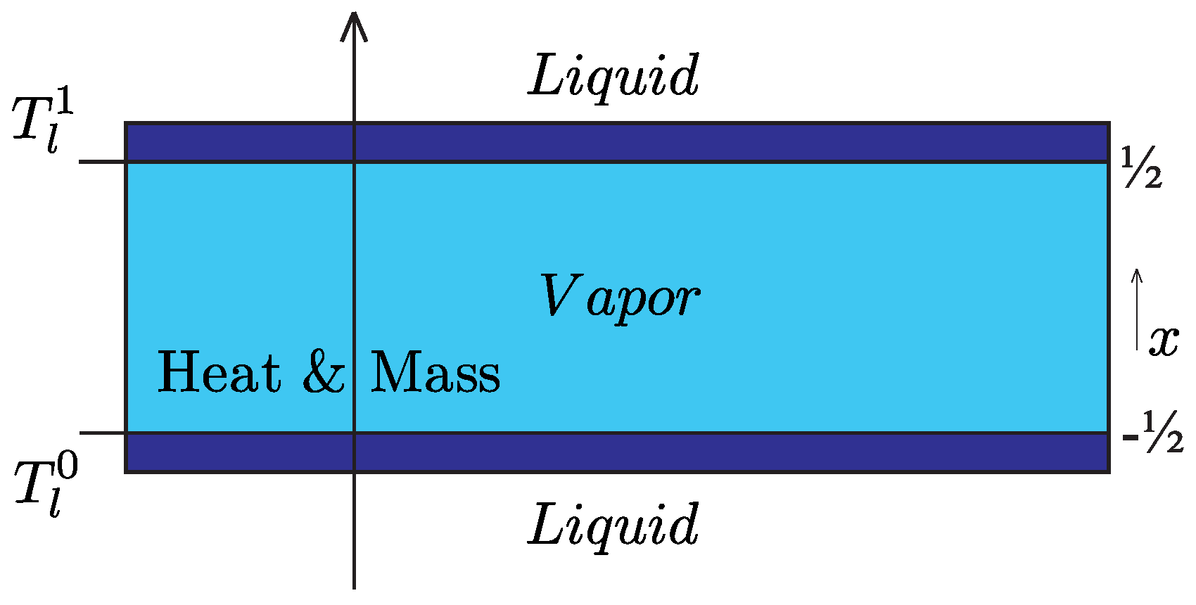
Figure 1.
System I: Vapour phase between two liquid reservoirs.
Figure 1.
System I: Vapour phase between two liquid reservoirs.
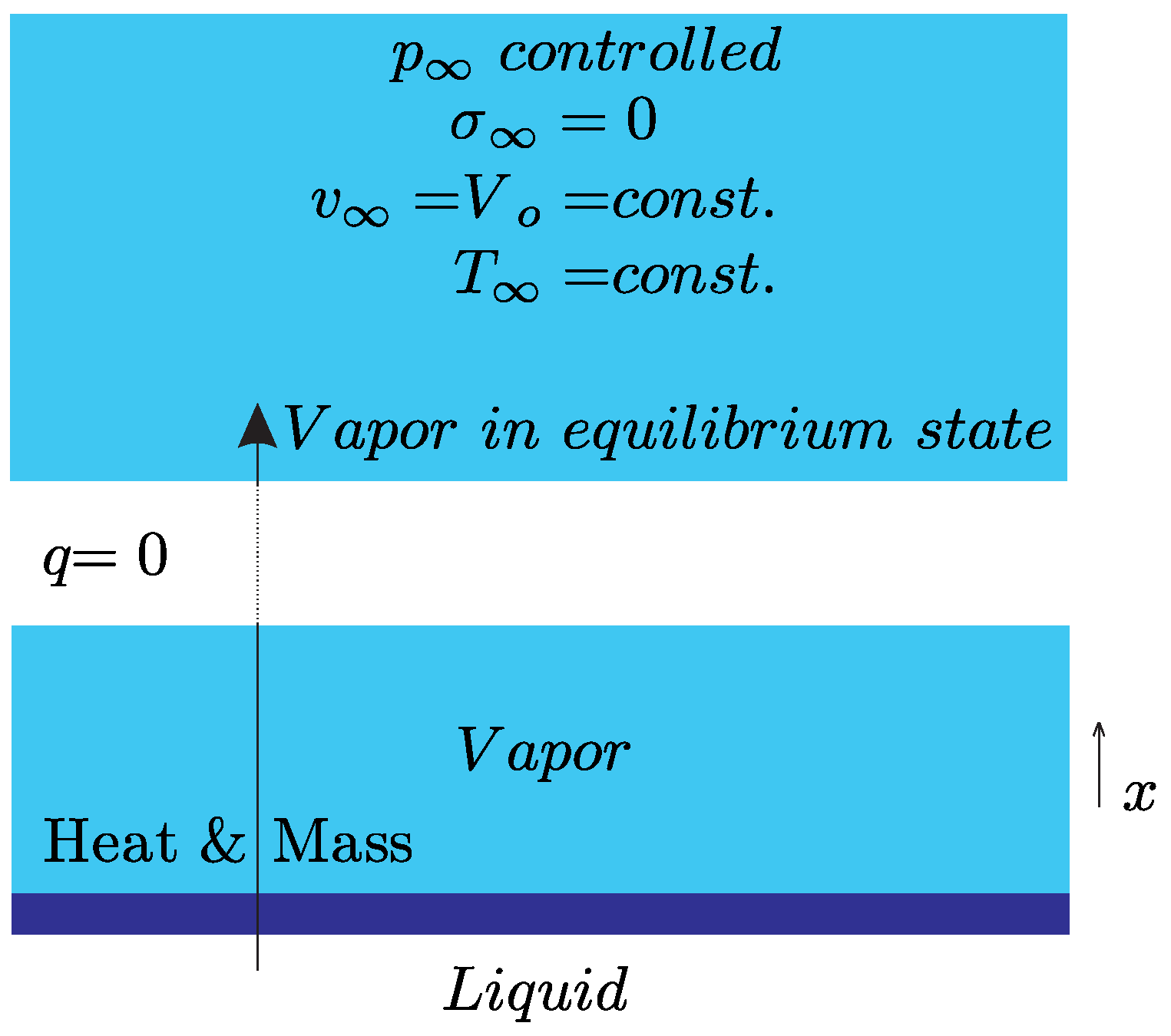
Figure 2.
System II: Half-space problem.
Figure 2.
System II: Half-space problem.
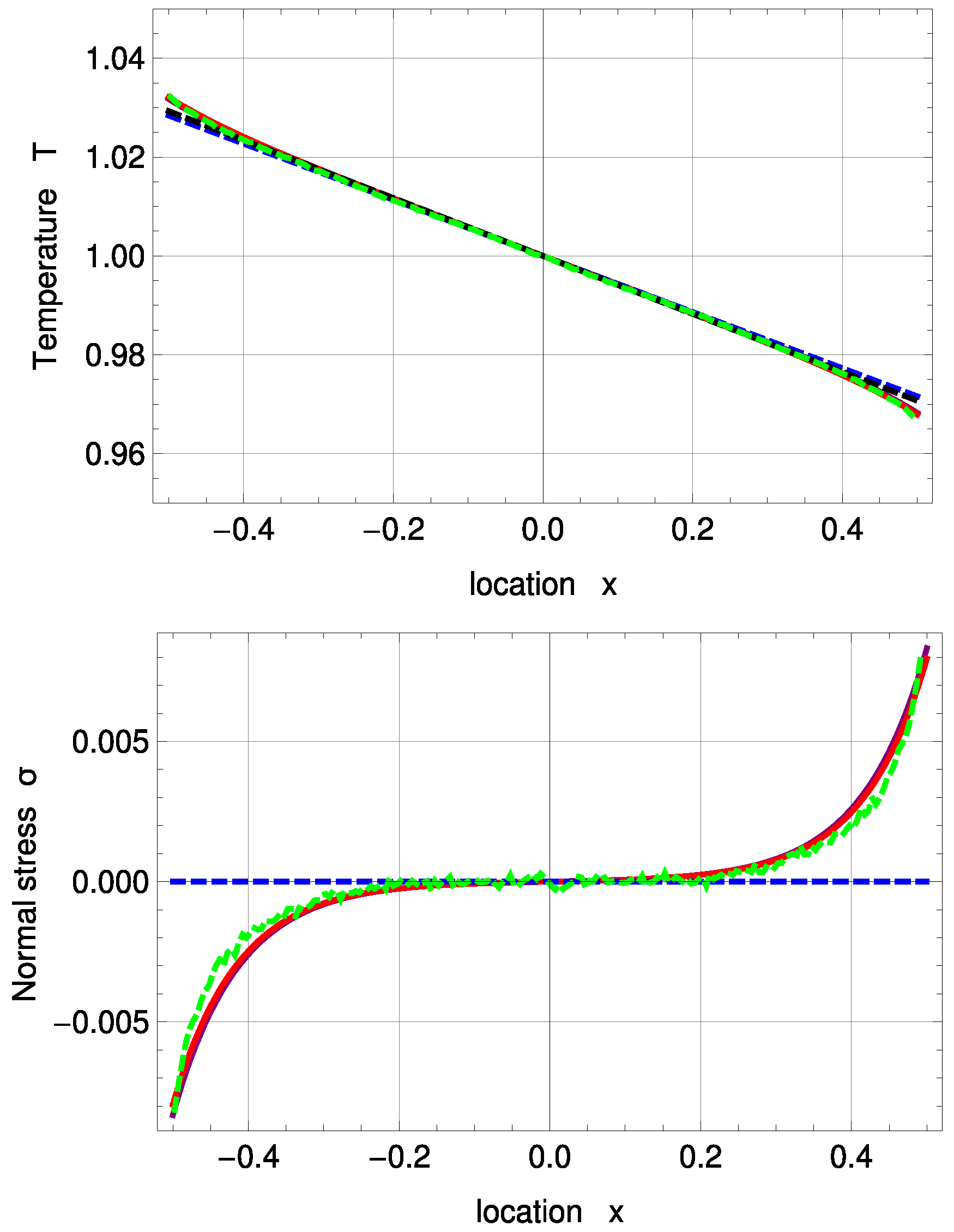
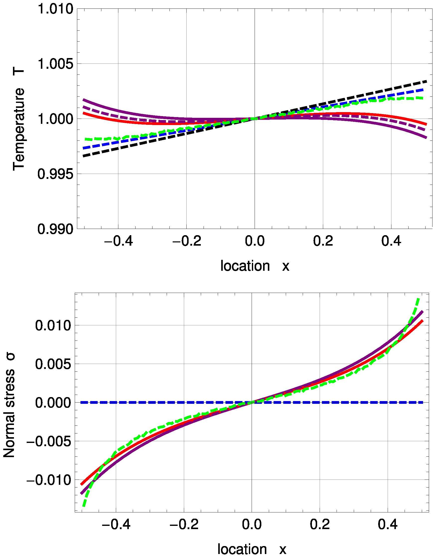
Figure 3.
Temperature and normal stress profiles for with and : Direct Simulation Monte Carlo method (DSMC) (symmetrized; green, dashed), R13 with PBC (purple), R13 with MBC (red), corrected NSF (blue, dashed), uncorrected NSF (black, dashed). Note: In the upper plot, all curves superimpose on each other. In the lower plot, both NSF models are zero.
Figure 4.
Temperature and normal stress profiles for with and : DSMC (symmetrized; green, dashed), R13 with PBC (purple), R13 with MBC (red), corrected NSF (blue, dashed), uncorrected NSF (black, dashed). Note: In the upper plot, all curves superimpose on each other. In the lower plot, both NSF models are zero.
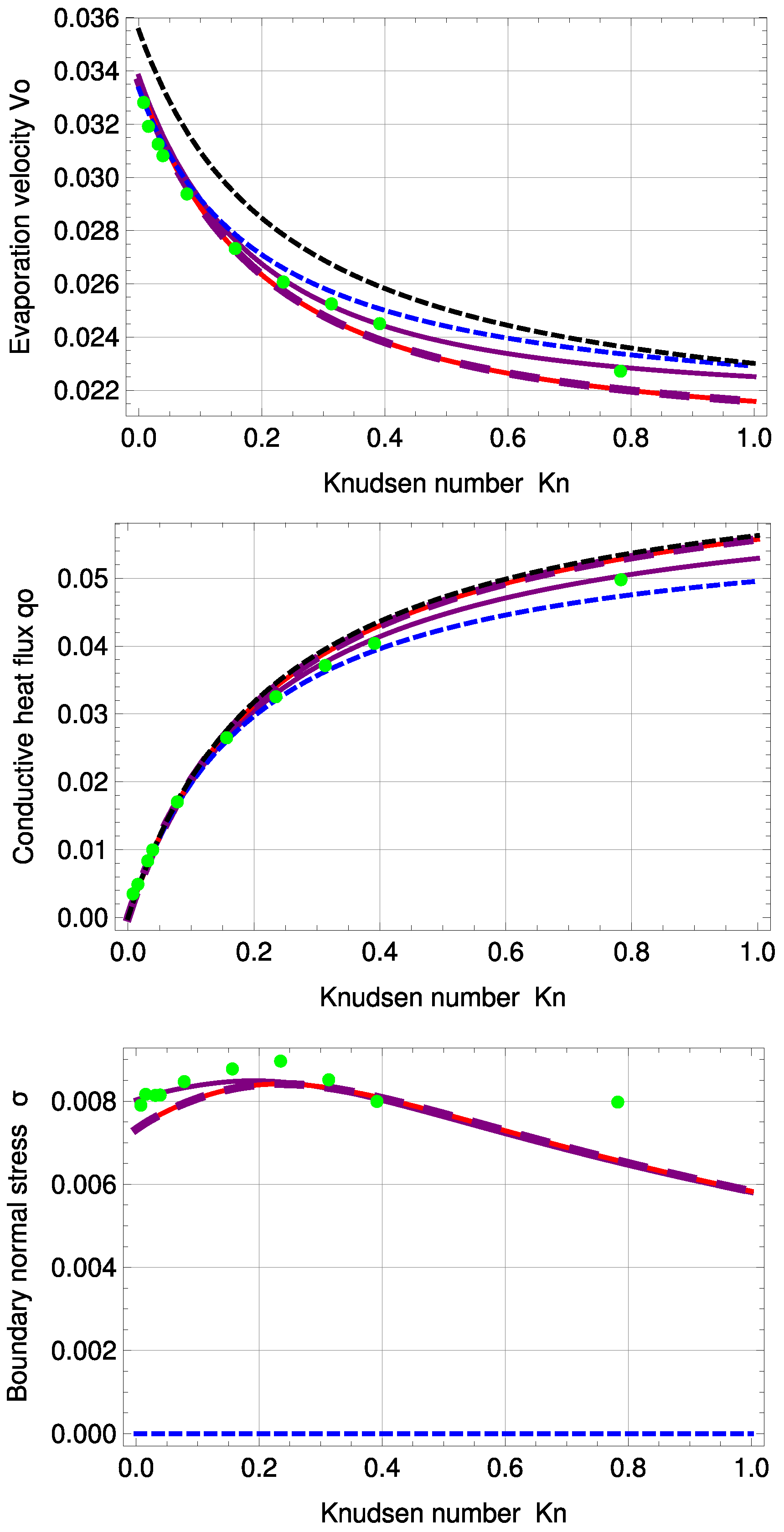
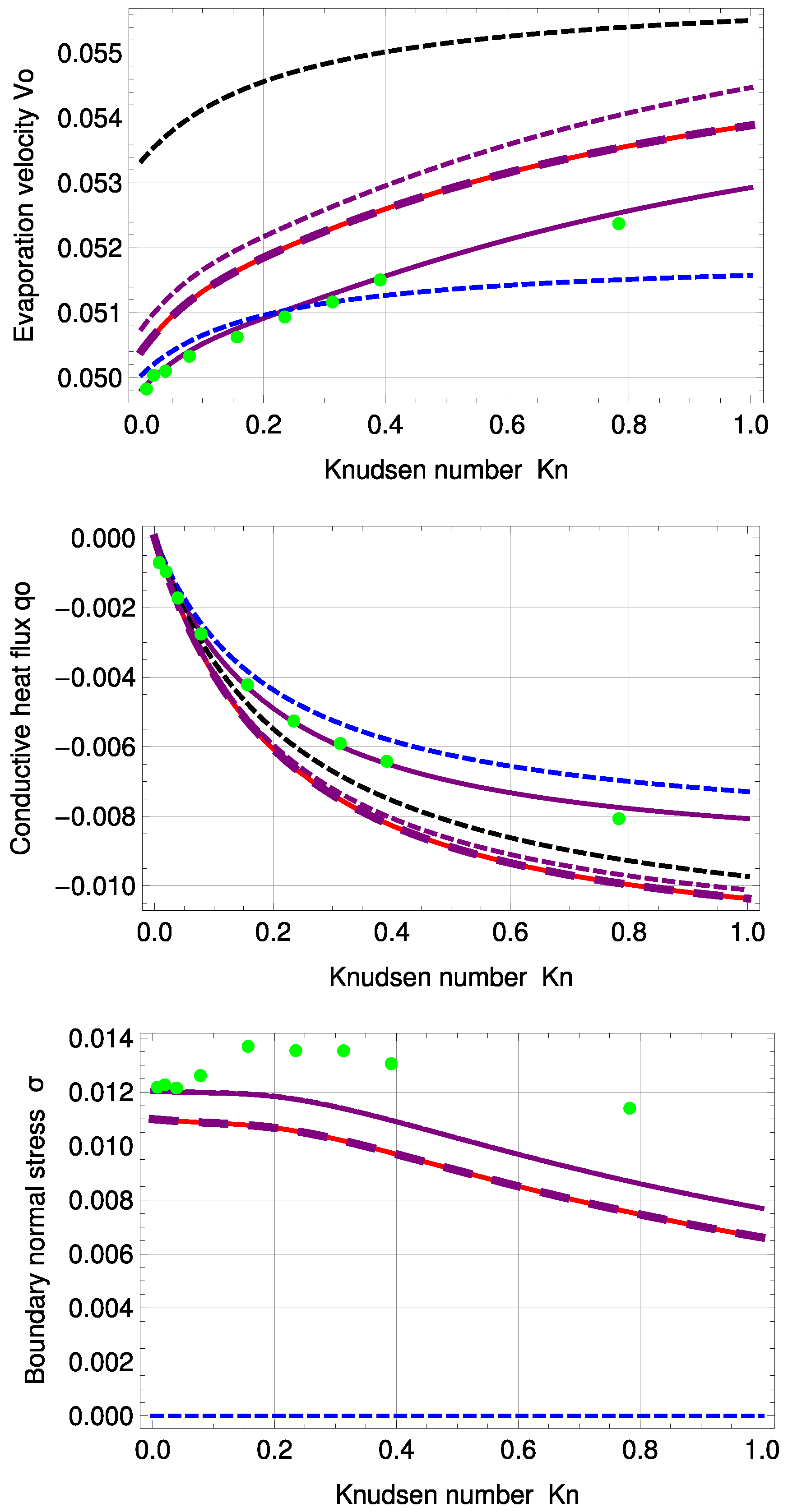
Figure 5.
Evaporation velocity , conductive heat flux and boundary normal stress for standard temperature profile: DSMC (green, dots), R13 with PBC (purple), R13 with PBC: (purple, large, dashed), R13 with MBC (red), corrected NSF (blue, dashed), uncorrected NSF (black, dashed).
Figure 5.
Evaporation velocity , conductive heat flux and boundary normal stress for standard temperature profile: DSMC (green, dots), R13 with PBC (purple), R13 with PBC: (purple, large, dashed), R13 with MBC (red), corrected NSF (blue, dashed), uncorrected NSF (black, dashed).
Figure 6.
Inverted temperature and normal stress profiles for with and : DSMC (symmetrized; green, dashed), R13 with PBC (purple), R13 with PBC and previous fitting (purple, dashed), R13 with MBC (red), corrected NSF (blue, dashed), uncorrected NSF (black, dashed).
Figure 6.
Inverted temperature and normal stress profiles for with and : DSMC (symmetrized; green, dashed), R13 with PBC (purple), R13 with PBC and previous fitting (purple, dashed), R13 with MBC (red), corrected NSF (blue, dashed), uncorrected NSF (black, dashed).
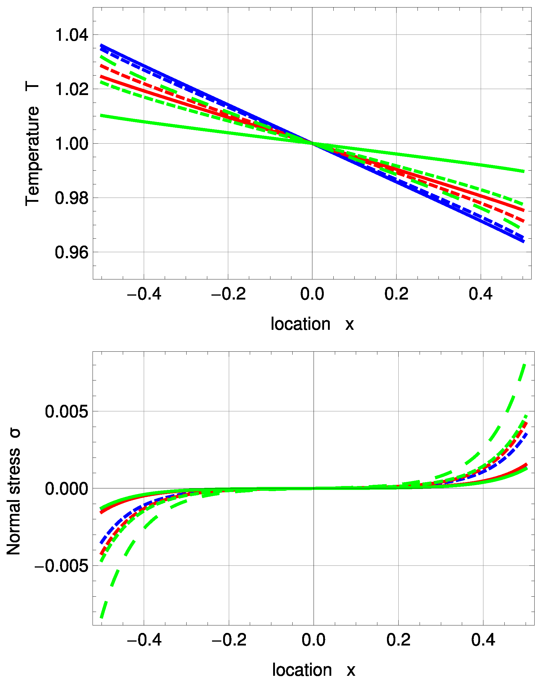
Figure 7.
Inverted temperature and normal stress profiles for with and : DSMC (symmetrized; green, dashed), R13 with PBC (purple), R13 with PBC and previous fitting (purple, dashed), R13 with MBC (red), corrected NSF (blue, dashed), uncorrected NSF (black, dashed).
Figure 7.
Inverted temperature and normal stress profiles for with and : DSMC (symmetrized; green, dashed), R13 with PBC (purple), R13 with PBC and previous fitting (purple, dashed), R13 with MBC (red), corrected NSF (blue, dashed), uncorrected NSF (black, dashed).
Figure 8.
Evaporation velocity , conductive heat flux and boundary normal stress for inverted temperature profile: DSMC (green, dots), R13 with PBC (purple), R13 with PBC: (purple, large, dashed), R13 with PBC and previous fitting (purple, dashed), R13 with MBC (red), corrected NSF (blue, dashed), uncorrected NSF (black, dashed). Note: For , the purple, dashed line is underneath the purple, solid line.
Figure 9.
PBC temperature and normal stress profiles for and various evaporation and accommodation coefficients: (green), (red), (blue), (solid), (dashed), (large, dashed). Note: For , the green, large dashed curve represents the solutions of all three .
Figure 9.
PBC temperature and normal stress profiles for and various evaporation and accommodation coefficients: (green), (red), (blue), (solid), (dashed), (large, dashed). Note: For , the green, large dashed curve represents the solutions of all three .
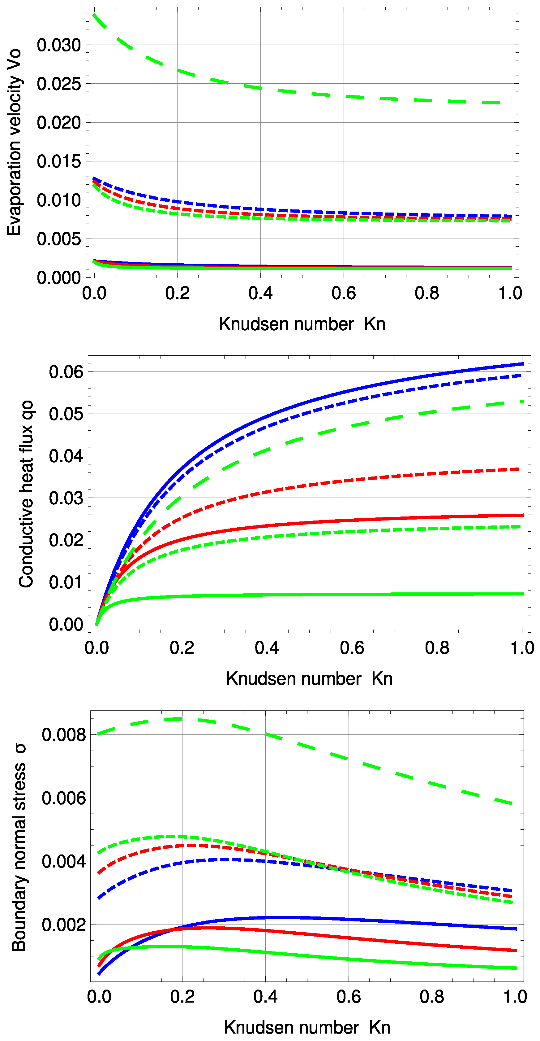
Figure 10.
PBC evaporation velocity , conductive heat flux and boundary normal stress for the standard temperature profile and various evaporation and accommodation coefficients: (green), (red), (blue), (solid), (dashed), (large, dashed). Note: For , the green, large dashed curve represents the solutions of all three .
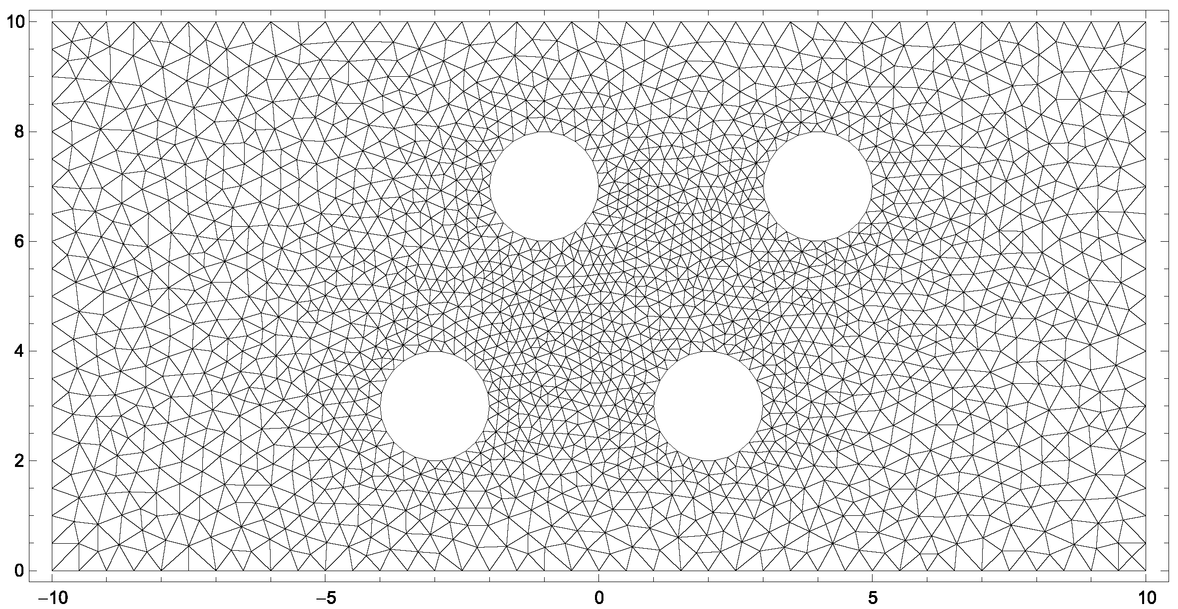
Figure 11.
Grid of two-dimensional channel-flow with four evaporating cylinders.
Figure 11.
Grid of two-dimensional channel-flow with four evaporating cylinders.
Figure 12.
Pressure contours superimposed by velocity streamlines for two-dimensional channel-flow with four evaporating cylinders and various Knudsen numbers.
Figure 12.
Pressure contours superimposed by velocity streamlines for two-dimensional channel-flow with four evaporating cylinders and various Knudsen numbers.
Figure 13.
Temperature contours superimposed by cond.heat flux streamlines for two-dimensional channel-flow with four evaporating cylinders and various Knudsen numbers.
Figure 13.
Temperature contours superimposed by cond.heat flux streamlines for two-dimensional channel-flow with four evaporating cylinders and various Knudsen numbers.
Table 1.
Coefficients for Maxwell (MM), Hard Sphere (HS) and Bhatnagar–Gross–Krook (BGK) models for the R13 equations.
Table 1.
Coefficients for Maxwell (MM), Hard Sphere (HS) and Bhatnagar–Gross–Krook (BGK) models for the R13 equations.
| | | | | Pr | Pr | Pr | Pr |
|---|
| MM | 2 | 3 | 45/8 | 2/3 | 7/6 | 3/2 | 2/3 |
| BGK | 2 | 2 | 5/2 | 1 | 1 | 1 | 1 |
| HS | 2.02774 | 2.42113 | 5.81945 | 0.6609 | 1.3307 | 1.3951 | 0.9025 |
Table 2.
Factors to adjust the Onsager coefficients of the Phenomenological Boundary Conditions (PBC) for the standard temperature profile.
Table 2.
Factors to adjust the Onsager coefficients of the Phenomenological Boundary Conditions (PBC) for the standard temperature profile.
| | a | b | c | d | e | f |
|---|
| PBC standard profile | 1.02 | 0.96 | 1.30 | 0.94 | 0.50 | 1.20 |
Table 3.
Solutions for Ytrehus’ ratios and percentual deviation to Ytrehus’ solution for the standard temperature profile. MBC, Macroscopic Boundary Conditions; NSF, Navier–Stokes–Fourier.
Table 3.
Solutions for Ytrehus’ ratios and percentual deviation to Ytrehus’ solution for the standard temperature profile. MBC, Macroscopic Boundary Conditions; NSF, Navier–Stokes–Fourier.
| | | % to Ytrehus | | % to Ytrehus |
|---|
| PBC standard profile | 2.0956 | 1.40 | 0.4875 | 10.02 |
| MBC | 2.1097 | 0.74 | 0.4894 | 10.44 |
| NSF | 1.9940 | 6.18 | 0.4431 | - |
| NSF corrected | 2.1254 | - | 0.4472 | 0.93 |
| Ytrehus | 2.1254 | - | 0.4431 | - |
Table 4.
Factors to adjust the Onsager coefficients of the PBC for the inverted profile.
Table 4.
Factors to adjust the Onsager coefficients of the PBC for the inverted profile.
| | a | b | c | d | e | f |
|---|
| PBC inverted profile | 0.983 | 0.83 | 1.30 | 0.87 | 0.50 | 1.20 |
Table 5.
Solutions for Ytrehus’ ratios and percentual deviation to Ytrehus’ solution for inverted profile.
Table 5.
Solutions for Ytrehus’ ratios and percentual deviation to Ytrehus’ solution for inverted profile.
| | | % to Ytrehus | | % to Ytrehus |
|---|
| PBC inverted profile | 2.1352 | 0.46 | 0.4657 | 5.11 |
| Ytrehus | 2.1254 | - | 0.44311 | - |
Table 6.
Derivation of boundary conditions by adjusting the Onsager coefficients.
Table 6.
Derivation of boundary conditions by adjusting the Onsager coefficients.
| | E Vapouration/Condensation | W All with Energy Transfer | I Inflow/Outflow |
|---|
| | 0 | |
| | 0 | 0 |
| | 0 | 0 |
| | | |
| | | 0 |
| | | 0 |
| | | |
| | | |
| | | |
| | | |
Table 7.
Overview of input parameters for the boundary conditions.
Table 7.
Overview of input parameters for the boundary conditions.
| | E Vapouration/Condensation | W All with Energy Transfer | I Inflow/Outflow |
|---|
| | − | |
| | | |
Table 8.
Input parameters for two-dimensional channel flow with four evaporating cylinders.
Table 8.
Input parameters for two-dimensional channel flow with four evaporating cylinders.
| | E Vapouration/Condensation | W All with Energy Transfer | I Inflow/Outflow |
|---|
| | − | |
| | | |


