Global Efficiency of Heat Engines and Heat Pumps with Non-Linear Boundary Conditions

Abstract

Analysis of global energy efficiency of thermal systems is of practical importance for a number of reasons. Cycles and processes used in thermal systems exist in very different configurations, making comparison difficult if specific models are required to analyze specific thermal systems. Thermal systems with small temperature differences between a hot side and a cold side also suffer from difficulties due to heat transfer pinch point effects. Such pinch points are consequences of thermal systems design and must therefore be integrated in the global evaluation. In optimizing thermal systems, detailed entropy generation analysis is suitable to identify performance losses caused by cycle components. In plant analysis, a similar logic applies with the difference that the thermal system is then only a component, often industrially standardized. This article presents how a thermodynamic “black box” method for defining and comparing thermal efficiency of different size and types of heat engines can be extended to also compare heat pumps of different apparent magnitude and type. Impact of a non-linear boundary condition on reversible thermal efficiency is exemplified and a correlation of average real heat engine efficiencies is discussed in the light of linear and non-linear boundary conditions.

1. Introduction

When optimizing a thermal plant, using a heat driven power cycle or a heat pump, practical experience indicates that one seldom have the luxury of choosing the components in any of the systems considered. Instead, the plant designer often needs to choose between preexisting, industrially standardized machines. Such preexisting thermal systems will have characteristics almost according to the designer’s preferences, but seldom exactly. Each of the potential thermal system will respond differently to optimizations of the plant. Unless the providers make a complete and unique model available of each potential thermal system, plant optimization has to rely heavily on assumptions. Since such unique models have a tendency to become biased, the problem remains regardless. We therefore propose a different approach to comparing thermal systems on a global level. Global in this approach means that the power cycle or heat pump is treated as a “black box” with global efficiency defined by the real boundary conditions dictated by the plant in which the “black box” operates.

A sound comparison of energy efficiency of thermal systems performing almost similar duty benefits not only from a “black box” approach, but also from a non-dimensional scale and an accurate definition of the reversible energy efficiency of each system. In this article, “thermal systems” means heat engines and heat pumps.

Black box approaches can be defined as independent of technology used. The importance of the black box approach is determined by its purpose. When comparing thermal systems using different cycles, there is no benefit in separating losses internal to the cycle from losses external to the cycle. By cycle design typical external losses, such as pinch-effects and impact of limited heat exchanger inventories, can be mitigated and are therefore linked to internal cycle losses in various ways. If the purpose instead is to study possible improvement potential of a particular cycle, then conventional second law analysis is highly effective. In such a case, there is no need for a black box approach.

In most practical cases, heat sources as well as heat sinks are finite. Therefore, exit temperatures from the thermal system vary depending on its energy efficiency. A small heat engine, relative to the apparent thermal capacity of source and sink, will operate at a larger temperature difference compared to a large system. Therefore, a comparison between thermal systems of different magnitude requires a measure indicating how small or large each system is relative to the boundary conditions of the heat source and sink. Furthermore, any variation in temperature difference means that an immediate comparison of energy efficiency becomes ambiguous. Instead comparison of energy efficiencies should relate to the reversible energy efficiency of each system, implicitly therefore also to the exit temperatures of the source and sink that would be obtainable using a thermodynamically perfect cycle.

Complexity is added by the fact that many thermal systems operate in environments where apparent heat capacity of heat source and/or heat sink are functions of temperature. We call them “complex”, or non-linear. If the apparent heat capacity is constant we call them “linear”. In the latter case, analytical formulas can be derived by defining reversible exit temperatures of source and sink as well as reversible energy efficiency. In the complex or non-linear cases, we need a numerical approach.

In the following, we will refer to methods of defining reversible energy efficiency of heat engines and we will propose the same method for comparison of heat pumps. Obviously, refrigeration systems can be compared in a similar manner as heat pumps.

Lorenz [1] defined a type of reversible cycles specifying how the temperatures in finite source and sink changed with transportation of heat through it. With such definition, reversible energy efficiency can be found analytically if the polytropes of the Lorenz cycle constitute equations suitable to integration. In many applications, for example, a heat engine using waste heat recovery of a diesel engine, however the polytropes become difficult to integrate.

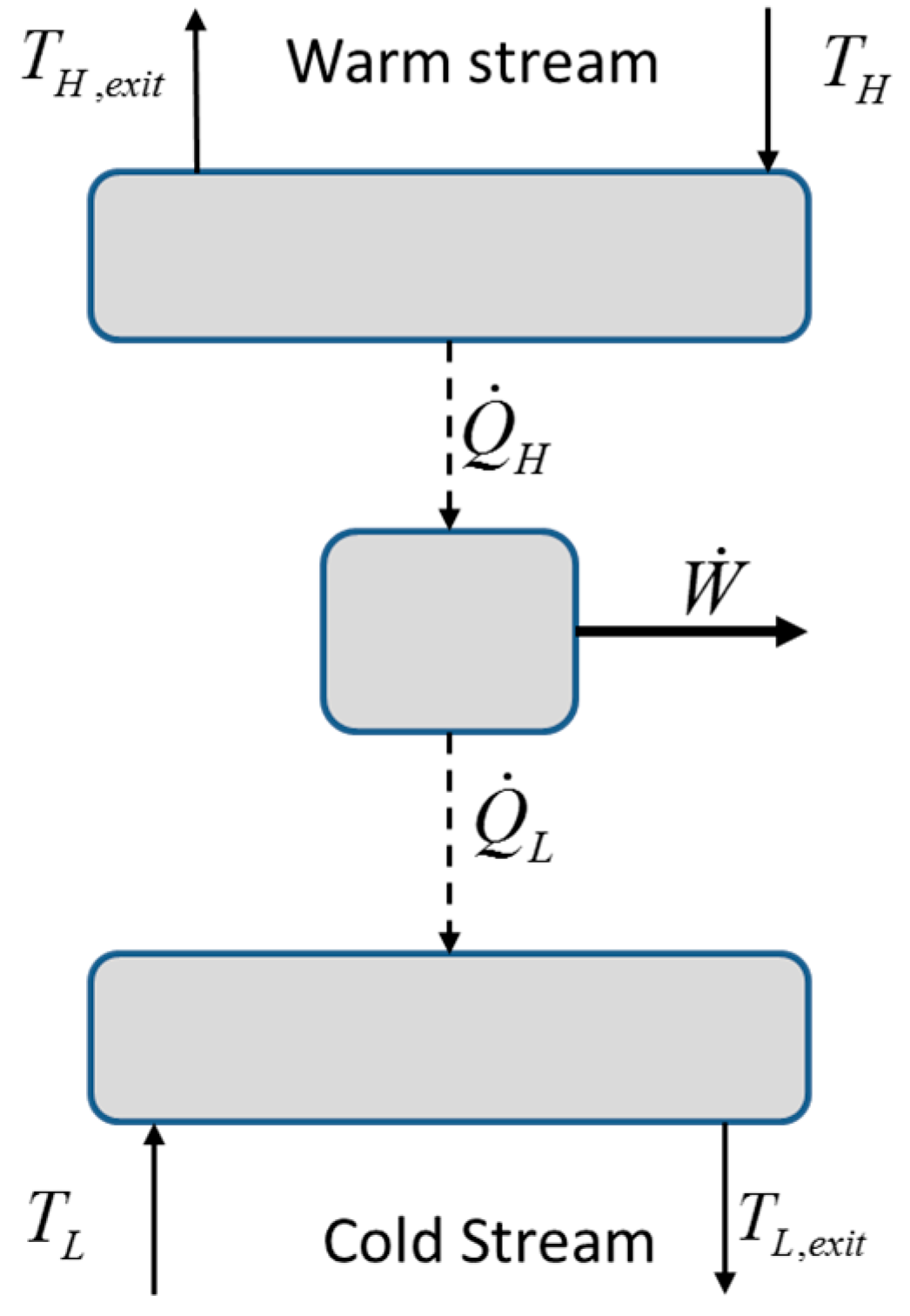
Ibrahim & Klein [2] showed a numerical definition of extractable work from a reversible cycle named the “max power cycle”. They used multiple, small, Carnot cycles in consecutive order relative to source and sink. In Öhman & Lundqvist [3] the concept of “Integrated Local Carnot Efficiency” ${\eta }_{C,Il}$ was defined as the reversible thermal efficiency of a max power cycle. Using Figure 1 we can extend the approach to also comprise heat pumps.

Equation (1) shows a definition of energy efficiency, or thermal efficiency, of a reversible heat engine.

$${\eta }_{th,s}={\dot{W}}_s/{\dot{Q}}_H$$

(1)

Consequently, we may define energy efficiency of a reversible heat pump in Equation (2), operating at the same temperatures.

$$CO{P}_s=1/{\eta }_{th,s}$$

(2)

As explained in Öhman & Lundqvist [4] we may use the approximation of Curzon–Ahlborn efficiency as of Curzon & Ahlborn [5] in Equation (3), to define the temperature that a source and a sink would equalize to by using a reversible heat engine as in Equation (4), the Curzon–Ahlborn temperature $T_{CA}$. Note however that, as explained in Öhman [6], using Curzon–Ahlborn efficiency limits the use of Equation (4) to applications with a linear source and sink. A generalization to complex sources and sinks requires the numerical solution of the max power cycle to determine this temperature.

$${\eta }_{CA}=1-\sqrt{T_L/T_H}$$

(3)

We wish to stress that the use of Equation (3) does not imply that the method described is developed according to the tradition of finite-time thermodynamics, FFT, or endo-reversible thermodynamics. It is only used as a simplification used to derive Equation (4) and only applicable to linear boundary conditions. Öhman [6] explains that Equation (3) is incorrect, however the error is small enough to allow its use in Equation (4) for determining Equation (5).

FTT, influenced by Curzon & Ahlborn [5] is a related field of science often focusing on cycle optimization and heat transfer in finite environments. Dong et al. [7] explain a general method to obtain optimal operating points for endo-reversible and irreversible heat engines. Ge et al. [8] explain the advances in finite-time thermodynamics for internal combustion cycle optimization. Feidt [9] explains the development in some traditions of thermodynamic analysis and that FTT is based on the idea of reversible cycle operating with irreversible heat exchange. Feidt [10] explains thermodynamic analysis of reverse cycles, clearly showing that FTT focuses on studying effects on thermal efficiency caused by explicit losses emanating from technical limitations. The black box approach focuses on thermal efficiency as a function of the magnitude of a thermal system relative to the source and sink, without assumptions on specific losses. From that reason, it is natural to use that approach also to study effects of complex boundary conditions. The method explained in this article is explicitly designed for simplified communication of the findings to practitioners.

2. Method

Using Equation (1) and the definition of inverse apparent heat capacity in the source as ${\alpha }_H=1/\left({\dot{m}}_H\cdot C{p}_H\right)$ and in the sink as ${\alpha }_L=1/\left({\dot{m}}_L\cdot C{p}_L\right)$, Öhman & Lundqvist [4] derived Equation (4) as follows. (Note the printing error in the equation in the reference.)

$$T_{CA}=\frac{T_L+T_H\cdot {\alpha }_L/{\alpha }_H\cdot \sqrt{T_L/T_H}}{1+{\alpha }_L/{\alpha }_H\cdot \sqrt{T_L/T_H}}$$

(4)

As extensively explained in Öhman [6], we can now define a dimensionless scale, named “utilization” and defined in Equation (5), on which to project the energy efficiency of a heat engine.

$$\psi ={\dot{Q}}_H/{\dot{Q}}_H\left(T_{CA}\right)={\dot{Q}}_H/{\dot{Q}}_{CA}$$

(5)

Note that ${\dot{Q}}_{CA}$ is only determined by the nature of the source and sink, while ${\dot{Q}}_H$ is the actual rate of heat entering the heat engine.

Now we can construct a diagram by plotting various characteristic data vs. “utilization” in a dimensionless way, thereby allowing comparison of heat engines of different magnitude relative to the finiteness of heat source and sink. This approach is suggested in Öhman [6] for the comparison of the global energy efficiency of different real heat engines. For the correlation of global energy efficiency of a real heat engine, it is possible to define a “Fraction of Carnot” (FoC) as of Equation (6). The FoC can be explained as measured, or simulated, using thermal efficiency divided by the ideally possible at the given utilization $\psi$, where $0\le \psi \le 1$.

$$FoC\left(\psi \right)={\eta }_{th}/{\eta }_{C,Il}\left(\psi \right)={\dot{W}}_{real}/{\dot{W}}_s\left(\psi \right)$$

(6)

Note that, by referring to boundary conditions of the reversible thermal system, FoC is not equivalent to common definitions of exergy efficiency. Note also that ${\eta }_{C,Il}\left(\psi \right)$, determined by the numerical max power cycle approach, can be easily validated for linear boundary conditions using equations available in standard literature. Appendix A in Öhman [6] provides explicit expressions for such validation.

3. Results

3.1. Global Efficiency of Heat Pumps

Thermodynamic entities of a reversible heat pump can be viewed as a symmetric mirror of a heat engine operating at the same conditions.

Figure 2 shows temperatures of source and sink for two different thermal systems. On the right side, temperatures of a reversible heat engine are indicated, cooling a hot flow from $T_H$ to $T_{H,exit}$ while heating a cold flow from $T_L$ to $T_{L,exit}$, If ${\dot{Q}}_H={\dot{Q}}_{CA}$ exit temperatures coincide. On the left side, temperatures of a reversible heat pump are indicated, heating a hot flow from $T_{H,exit}$ to $T_H$ while cooling a cold flow from $T_{L,exit}$ to $T_L$. If $T_{H,exit}\ne T_{L,exit}$ a fictitious heat pump equilibrium temperature can be constructed in the same way as at $T_{CA}$ in Equation (4) for linear boundary conditions and from the numerical model for complex boundary conditions. We can therefore use Equations (5) and (7) to determine utilization.

$${\dot{Q}}_{CA}=\frac{T_H-T_{H,exit}}{{\alpha }_H}$$

(7)

We can understand that the temperatures in Figure 2 will be symmetric around ${\dot{Q}}_H=0$ by the analogy of the max power cycle and its use of multiple subsequent very small Carnot Cycles. Carnot Cycles are reversely applicable to heat engines and heat pumps.

Öhman [6] proposed Equation (8) as the expected correlated global energy efficiency of real low temperature difference heat engines.

$$FoC\left(\psi \right)=0.672\cdot e^{-0.874\cdot \psi }$$

(8)

Equation (8) is based on measured global energy efficiency for heat engines in a very large range of capacities, temperatures, and technical solutions. Yet, it is remarkably consistent. It allows us very expediently to predict thermal efficiency as well as output power of an undefined real heat engine by using Equation (6), only knowing the characteristics of a particular set of sources and sinks if the utilization is known. The correlation describes an average of historic data and could be seen as normal to industrial capability as of today.

Evaluating heat pump systems can be made in a similar manner as of the above by defining Equation (9) as a Fraction of Carnot for real heat pumps.

$$Fo{C}_{COP}\left(\psi \right)=CO{P}_{real}/CO{P}_s\left(\psi \right)={\eta }_{C,Il}\left(\psi \right)\cdot CO{P}_{real}$$

(9)

A correlation of $Fo{C}_{COP}\left(\psi \right)$ has not yet been attempted, but is intended to be performed once enough data has been gathered. It is clear however that global energy efficiency of heat pumps operating in non-identical applications can be systematically compared using the above approach.

3.2. Effects of Complex Boundary Conditions

As explained the simple approximation of Equation (3), and therefore also Equation (4) cannot be applicable if source flow and/or sink flow are complex/non-linear. Utilization can however still be defined by using the local temperatures calculated in the max power cycle. Figure 2 will look significantly different in such a case. Therefore, it is not to be expected that the correlation in Equation (8) is valid for complex boundary conditions.

In reality, complex boundary conditions are common and do require more detailed studies. The approach of the max power cycle, Integrated Local Carnot efficiency and Fraction of Carnot are useful in such studies. The following simplified example can be used to remind us that complex conditions cannot easily be regarded as approximately linear.

3.3. A Demonstrational Example

A demonstrational example can be constructed by applying a heat pump to heat a flow of air by cooling another flow of saturated humid air. A technical application could be a blast drying process or similar and thermally defined as of

Table 1. Input information for a demonstrational example.

Entity	Value	Unit
Hot air flow	3.33	kg/s
Hot air exit temp	80 (dry)	°C
Hot air entry temp	60	°C
Cp (hot air)	1	kJ/kg·K
${\alpha }_{heatedairflow}$	0.3	K/kW
Cold air flow	1.67	kg/s
Cold air entry temp	34 (saturated)	°C
Cp (cold air >34 °C)	1	kJ/kg·K
C (cold air <34 °C)	Equation (10)	kJ/kg·K
${\alpha }_{cooledair}$ Complex	$C\left(T_{cooledair}\right)$ Equation (10)	K/kW
${\alpha }_{cooledair}$ Linear	0.6	K/kW

.

The specific heat of the cold air is here modeled in two ways; (i) linear, meaning that Cp is constant and that ${\alpha }_{cooledair}$ is consequently also constant; (ii) complex, meaning that Cp is constant above 34 °C and a function of temperature as of Equation (10) below 34 °C. The reason for the complexity is the condensation of water as the cold air is further cooled below 34 °C. Equation (10) is a polynomial approximation of dh/dT for condensing humid air per mass unit of dry air calculated in the commercial software EES (Engineering Equations Solver) with data on air from Lemmon et al. [11] and data on H₂O from Hyland & Wexler [12].

$$C\left(T\right)=0.0026\cdot T^3-0.0934\cdot T^2+3.5776\cdot T+2.6929$$

(10)

Using the set of data from Table 1 we can apply the numerical approach of the max power cycle to obtain the fictitious $T_{CA}$, output temperature of the cold stream, Utilization, Integrated Local Carnot efficiency and COP for a reversible heat pump for the linear cold stream as well as for the complex cold stream. Net calculated data can be found in

Table 2. Calculated data for a reversible blast heater.

Entity	Value	Unit
Hot flow heating	66.7	kW
Reversible COP, complex	8.7	-
Reversible COP, linear	6.5	-
Cold flow exit temp, complex	27	°C
Cold flow exit temp, linear	0.3	°C
Utilization	0.69	-

.

By comparing the two alternative cold stream characteristics, it becomes obvious that a non-linear, or complex cold stream leads to a difference in reversibly obtainable COP by roughly 30% as compared to assuming a linear cold stream. Figure 3 shows the local temperatures during the two processes. Note that this difference in COP is at reversible conditions. Any measured COP of a real system should be compared to the correct COP, taking the complex nature of the heat sink into account.

The temperature diagrams in Figure 3 clearly shows why Integrated Local Carnot efficiency must differ between the two processes. Due to the large difference in apparent heat capacity in the cold stream when condensation occurs the necessary temperature lift in the heat pump becomes smaller. This leads to a lower Integrated Local Carnot efficiency and a larger COP for the reversible heat pump.

This example indicates why a correlation similar to Equation (8), but for heat pumps, is not likely to be valid in applications with complex boundary conditions.

4. Discussion

The explained method uses conventional thermodynamic entities to create a dimensionless comparative method for black box energy efficiency. It comprises first as well as second law effects. Other methods can be used but are likely to become more complicated. The numerical approach of the max power cycle provides the benefit of detailed information about local temperatures in source and sink and thereby greatly simplifies the understanding of pinch points and similar effects.

The use of detailed exergy destruction analysis is constructive in identifying and evaluating irreversibility. However, when determining reversible thermal efficiency exergy efficiency becomes meaningless. The approach of Integrated Local Carnot efficiency is a direct implementation of multiple Carnot cycles hence it can be directly derived by assuming zero increase of entropy.

With a similar, systematic black box approach, for heat engines and heat pumps, experiences from one type of thermal system may be useful to understand effects of another.

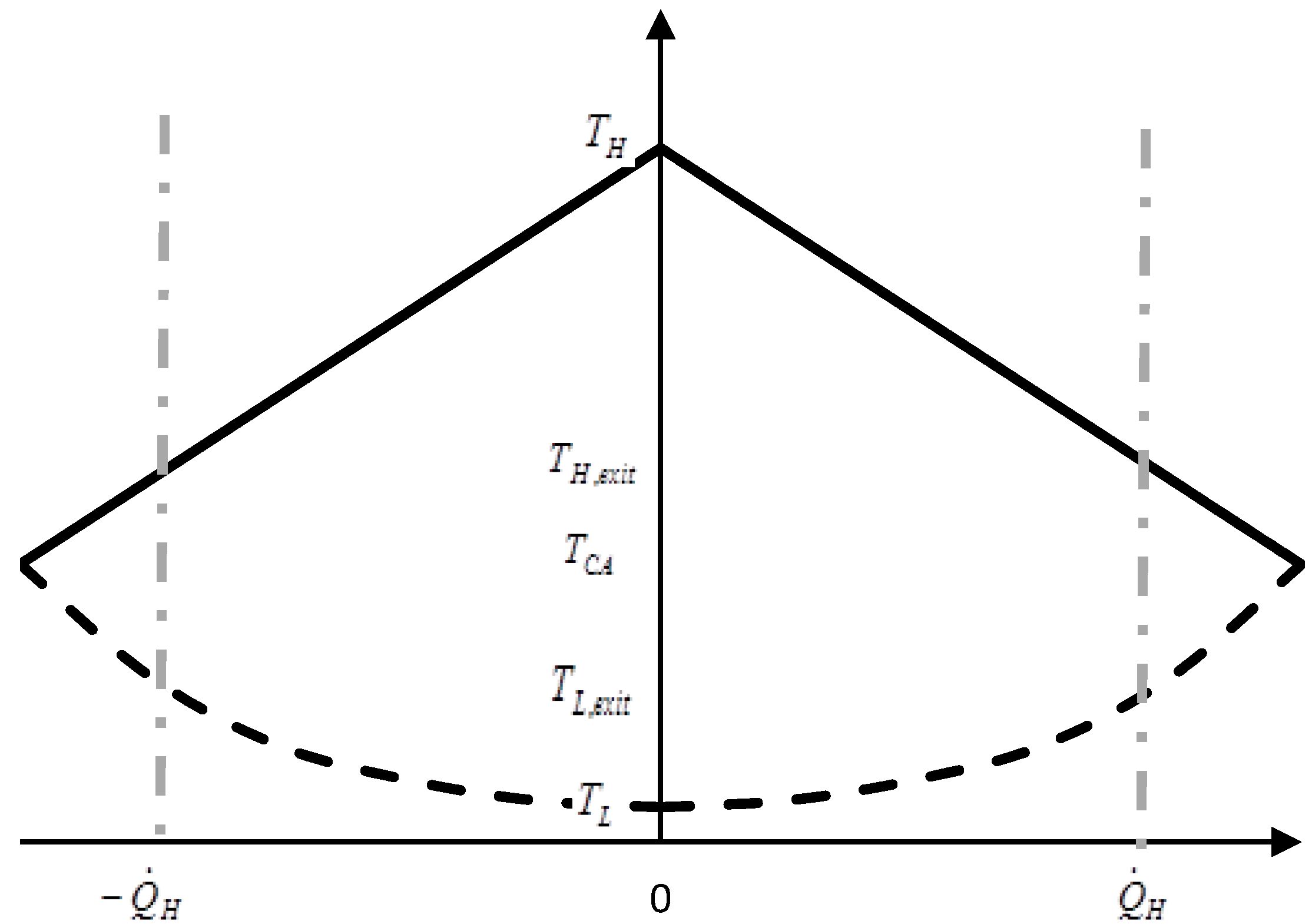
A particularly interesting question arises when using the concept of utilization for heat engines and heat pumps in a symmetric manner, such as in Figure 2. A research question arising from this discussion is if a correlation, similar to Equation (8) could be found for heat pumps or cooling systems. We suggest researching real heat pump thermal efficiency for further studies using the method described in this article.

5. Conclusions

We have shown that a black box method for investigating efficiency of low temperature heat engines explained in Öhman [6] can be extended to apply also to heat pumps.

The dimensionless scale of utilization can be used for systematic comparison of thermal efficiency of heat engines as well as heat pumps with different magnitudes relative to the source and sink.

The max power cycle approach of Ibrahim & Klein [2] is suitable to determine reversible thermal efficiency of a thermal system with complex boundary conditions.

There may be significant impact of complex boundary conditions on reversible thermal efficiency of a thermal system.

References

1. Lorenz, H. Beiträge zur Beurteilung von Kuhlmaschinen. Z. Ver. Dtsch. Ing. 1894, 38, 63–68. (In German) [Google Scholar]
2. Ibrahim, O.M.; Klein, S.A. Absorption power cycles. Energy 1996, 21, 21–27. [Google Scholar] [CrossRef]
3. Öhman, H.; Lundqvist, P. Theory and method for analysis of low temperature driven power cycles. Appl. Therm. Eng. 2012, 37, 44–50. [Google Scholar] [CrossRef]
4. Öhman, H.; Lundqvist, P. Comparison and analysis of performance using Low Temperature Power Cycles. Appl. Therm. Eng. 2013, 52, 160–169. [Google Scholar] [CrossRef]
5. Curzon, F.L.; Ahlborn, B. Efficiency of a Carnot Engine at Maximum Power Output. Am. J. Phys. 1975, 43, 22–24. [Google Scholar] [CrossRef]
6. Öhman, H. Low Temperature Difference Power Systems and Implications of Multiphase Screw Expanders on Organic Rankine Cycles. Ph.D. Thesis, KTH Royal Institute of Technology, Stockholm, Sweden, 2 September 2016. [Google Scholar]
7. Dong, Y.; El-Bakkali, A.; Descombes, G.; Feidt, M.; Perilhon, C. Association of Finite-Time Thermodynamics and a Bond-Graph Approach for modeling an endoreversible heat engine. Entropy 2012, 14, 642–653. [Google Scholar] [CrossRef]
8. Ge, Y.; Chen, L.; Sun, F. Progress in Finite Time Thermodynamic studies for internal combustion engine cycles. Entropy 2016, 18, 139. [Google Scholar] [CrossRef]
9. Feidt, M. Optimal thermodynamics—New upperbounds. Entropy 2009, 11, 529–547. [Google Scholar] [CrossRef]
10. Feidt, M. Thermodynamics applied to reverse cycle machines, a review. Int. J. Refrig. 2010, 33, 1327–1342. [Google Scholar] [CrossRef]
11. Lemmon, E.W.; Jacobsen, R.T.; Pennoncello, S.G.; Freiend, D.G. Thermodynamic properties of air and mixtures of nitrogen, argon, and oxygen from 60 to 2000 K at pressures to 2000 MPa. J. Phys. Chem. Ref. Data 2000, 29, 331–385. [Google Scholar] [CrossRef]
12. Hyland, R.; Wexler, A. Formulations for the thermodynamic properties of the saturated phases of H2O from 173.15 K to 473.15 K. ASHRAE Trans. 1983, 89, 500–519. [Google Scholar]
Figure 1. A principal heat engine or, if reversed a heat pump.
Entropy 19 00394 g001
Figure 2. Schematic local temperatures of the hot and the cold streams in a heat pump and a heat engine vs. transported heat (Utilization). Negative rate of heat means heat pump, positive rate of heat means heat engine.
Entropy 19 00394 g002
Figure 3. Local temperatures, in °C, of the hot and two alternative cold streams during the two alternative processes as a function of utilization. The calculated processes both start at utilization −0.69 since the heat capacity of the two alternative cold streams are equal when temperature would be above 34 °C. Note that negative utilization indicates a heat pump.
Entropy 19 00394 g003