Hypothesis Tests for Bernoulli Experiments: Ordering the Sample Space by Bayes Factors and Using Adaptive Significance Levels for Decisions

Abstract

The main objective of this paper is to find the relation between the adaptive significance level presented here and the sample size. We statisticians know of the inconsistency, or paradox, in the current classical tests of significance that are based on p-value statistics that are compared to the canonical significance levels (10%, 5%, and 1%): “Raise the sample to reject the null hypothesis” is the recommendation of some ill-advised scientists! This paper will show that it is possible to eliminate this problem of significance tests. We present here the beginning of a larger research project. The intention is to extend its use to more complex applications such as survival analysis, reliability tests, and other areas. The main tools used here are the Bayes factor and the extended Neyman–Pearson Lemma.

1. Introduction

Recently, the use of $p$-values in tests of significance has been criticized. The question posed in [1] and discussed in [2,3,4] concerns the misuse of canonical values of significance level (0.10, 0.05, 0.01, and 0.005). More recently, a publication by the American Statistical Association [5] makes recommendations for scientists to be concerned with choosing the appropriate level of significance. Pericchi and Pereira [6] consider the calculation of adaptive levels of significance in an apparently successful solution for the correction of significance level choices. This suggestion eliminates the risk of a breach of the likelihood principle. However, that article deals only with simple null hypotheses, although the alternative may be composite. Another constraint is the dimensionality of the parameter space; the article was only about one-dimensional spaces. More recent is the article by 72 prominent scientists [7], as described on the website of Nature Human Behavior [8]. In a genuinely Bayesian context, the authors of [9] introduced the index e (e-value, e for evidence) as an alternative to the classical p-value, which we write with a lower-case “$p$”. A correction to make the null hypothesis invariant under transformations was presented in [10], and a more theoretical review can be seen in [11,12]. The e-value was the basis of the solution of an astrophysical problem described in [13]. The relationship between p-values and e-values is discussed in [14]. However, while the e-value works for hypotheses of any dimensionality without needing assignment of “point mass” probabilities to hypotheses of lower dimensionality than the parameter space, setting its significance level is not an easy task. This has made us look for a way to obtain a significance index that allows us to better understand how to obtain the optimal (in the sense we explain later) significance level of a problem of any finite dimensionality. This work is based on four previous works [15,16,17,18]. It has taken a long time to see the possibility of using them in combination and with reasonable adjustments: the Bayes factor takes the place of the likelihood ratio and the average value of the likelihood function replaces its maximum value. The mean of the likelihood function under the null hypothesis will be the density used in the calculation of the new index, the $P$-value, which we represent with a capital “P” to differentiate it from the classical $p$-value. The basis of all our work is the extended Neyman–Pearson Lemma in its Bayesian form (see [19], sections “Optimal Tests” (Theorem 1) and “Bayes Test Procedures” (pp. 451–452)).

We present here a new hypothesis testing procedure that can eliminate some of the major problems associated with currently used hypothesis tests. For example, the new tests do not tend to reject all hypotheses in the many-data limit like Neyman–Pearson tests do, nor do they tend to fail to reject all hypotheses in the same limit, like Jeffreys’s Bayesian (Bayes factor) hypothesis tests do.

2. Blending Bayesian and Classical Concepts

2.1. Statistical Model

As usual, let $x$ and $\theta$ be random vectors (could be scalars) $x$ ∈$\mathit{X}$ ⊂ ${\mathcal{R}}^{\mathit{s}}$, $\mathit{X}$ being the sample space, and $\theta \in \Theta \subset {\mathcal{R}}^{\mathit{k}}$, $\Theta$ being the parameter space, and $s$ and $k$ being positive integers. To state the relation between the two random vectors, the statistician considers the following: a family of probability density functions indexed by the conditioning parameter$\theta , \left\{f\left(x|\theta \right);\theta \in \Theta \right\}$; a prior probability density function $g\left(\theta \right)$ on the entire parameter space$\Theta$, and the posterior density function $g\left(\theta |x\right).$ In order to be appropriate, the family of likelihood functions indexed by $x$, $\left\{L\left(\theta |x\right)=f\left(x|\theta \right);x\in \mathit{X} \right\},$ must be measurable in the prior σ-algebra.

With the statistical model defined, a partition of the parameter space is defined by the consideration of a null hypothesis that is to be compared to its alternative:

$$H:\theta \in {\Theta }_H \mathrm{and} A:\theta \in {\Theta }_A, \mathrm{where} {\Theta }_H{{\displaystyle \cup }}^{}{\Theta }_A=\Theta \mathrm{and} {\Theta }_H{{\displaystyle \cap }}^{}{\Theta }_A=\varnothing .$$

(1)

In the case of composite hypotheses with the partition elements having the same dimensionality, the model would then be complete. Such cases would not involve partitions for which there are components of zero Lebesgue measure. In the case of precise or “sharp” hypotheses, that is, the partition components having different dimensionalities, other elements must be added:

• positive probabilities of the hypotheses, $\mathsf{\pi }\left(H\right)>0 \mathrm{e} \mathsf{\pi }\left(A\right)=1-\mathsf{\pi }\left(H\right)>0;$ and
• a density on the subset that has the smaller dimension. The choice of this density should be coherent with the original prior density over the global parameter space$\Theta$.

Consider the common case for which the null hypothesis is the one defined by a subset of lower dimensionality. In this case, we use a surface integral to normalize the values of the prior density in the null set so that the sum or integral of these values is equal to unity. Figure 1 illustrates how this procedure is carried out. Recall that a prior density can be seen as a preference system in the parameter space. That preference system must be kept even within the null hypothesis; coherence in access to prior distributions is crucial. Further details on this procedure can be found in [16,17,18]. Later, Dawid, and Lauritzen [20] considered multiple ways of obtaining compatible priors under alternative models (hypotheses). The “conditioning” approach described by Dawid and Lauritzen is equivalent to the technique presented here. Dickey [21] used a similar approach previously, but in a more parameterization-dependent way.

Figure 1. A prior$g\left(p,q\right)$ made of independent $Beta\left(2,4\right)$ and $Beta\left(4,2\right)$ distributions in a two-dimensional parameter space is cut along the line $p=q$ and one of the pieces moved away to show the resulting prior on the lower-dimensional set$p=q$.

2.2. Significance Index

By “significance index”, we mean a real function over the sample space that is used as an evidence measure for decision-making with respect to accepting or rejecting the null hypothesis, H. We begin this section by stating a generalization of the Neyman–Pearson Lemma, as presented by DeGroot [19]. Cox [22,23] also considers the classical $p$-value as an evidence measure, and Evans [24] considers evidence measures in general, outlines the relative belief theory developed in the references of that paper, and suggests that the associated evidence measure could have advantages over other measures of evidence and be the basis of a complete approach to estimation and hypothesis-assessment problems. The classical $p$-value is the most widely used significance index across diverse fields of study, including almost all scientific areas. In the present work, we present a replacement for the classical $p$-value has a number of advantages that will be described here and in future work. The conceptual and operational similarity between classical hypothesis tests as currently used and the new tests could potentially help researchers accept and use the new tests.

Let $f_H\left(x\right) \mathrm{and} f_A\left(x\right)$ be probability density functions over the sample space$\mathit{X}$. The decision problem is to choose one of these densities as being the true generator of the observed data. Consider now a binary function $\delta \left(x\right)$ used to define the decision procedure. Defining a partition of the sample space with ${\mathit{X}}_H{{\displaystyle \cup }}^{}{\mathit{X}}_A=\mathit{X}$ and${\mathit{X}}_H{{\displaystyle \cap }}^{}{\mathit{X}}_A=\varnothing$, where${\mathit{X}}_H$ is the non-rejection region for H. The test function is

$$\delta \left(x\right)=\{\begin{array}{c}0,\hspace{1em}\mathrm{if} x\in {\mathit{X}}_H\hfill \\ 1,\hspace{1em}\mathrm{if} x\in {\mathit{X}}_A \hfill \end{array}.$$

(2)

To choose between a hypothesis and its alternative, one should first choose two positive real numbers, say$A \mathrm{and} B$, with $A>B,A=B \mathrm{and} A<B$ meaning, respectively, preference for the null hypothesis, indifference, and preference for the alternative. The decision rule is then to reject the null hypothesis,$H$, whenever$\delta \left(x\right)=1$, and not to reject otherwise. The following theorem, a generalized version of the Neyman–Pearson Lemma presented in the textbook by DeGroot [19] provides a test that is optimal in the sense of minimizing a linear combination of the probabilities of the two types of errors: Type I, which is the rejection of a true hypothesis, and Type II, the non-rejection of a false hypothesis.

$$\alpha \left(\delta \right)=\mathrm{Pr}\left\{\mathrm{rejecting} H|H \mathrm{is} \mathrm{true}\right\}=\mathrm{Pr}\left\{\delta \left(x\right)=1|H\right\}$$

(3)

and

$$\beta \left(\delta \right)=\mathrm{Pr}\left\{\mathrm{not} \mathrm{rejecting} H|H \mathrm{is} \mathrm{false}\right\}=\mathrm{Pr}\left\{\delta \left(x\right)=0|A\right\}.$$

(4)

Generalized Neyman–Pearson Lemma:

Let ${\delta }^{*}$ be a test that rejects H in favor of A if $A{f}_H\left(x\right)< B{f}_A\left(x\right)$, does not reject H if $A{f}_H\left(x\right)> B{f}_A\left(x\right)$, and is indifferent if $A{f}_H\left(x\right)=B{f}_A\left(x\right).$ Then, for any other test $\delta ,$

$$A\alpha \left(\delta \right)+B\beta \left(\delta \right)\ge A\alpha \left({\delta }^{*}\right)+B\beta \left({\delta }^{*}\right).$$

(5)

In 1957, both Lindley [25] and Bartlett [26] recognized that fixing a significance level was a major cause of problems with hypothesis tests. In 1966, Cornfield [27] advocated hypothesis tests that minimize a linear combination of error probabilities like Equation (5) rather than fixing a canonical $\alpha$ and minimizing $\beta ,$ like in the Neyman–Pearson approach [28].

To see that Bayesian hypothesis tests minimize a linear combination of error probabilities of the form $A\alpha \left(\delta \right)+B\beta \left(\delta \right),$ consider a loss function that is zero if the decision is correct and $w_{\mathrm{A}} \left(w_{\mathrm{H}}\right)$ if the decision favors $A \left(H\right)$ when $H \left(A\right)$ is the true state of nature. In addition, if $\mathsf{\pi }$ is the prior probability of $H$ and $\delta$ the test function, the risk function is

$$\mathit{r}\left(\delta \right)=w_A\mathsf{\pi }\alpha \left(\delta \right)+w_H\left(1-\mathsf{\pi }\right)\beta \left(\delta \right).$$

(6)

Consequently, simply identifying$\left(\mathsf{\pi }{w}_{\mathrm{A}}\right) \mathrm{and} \left(1-\mathsf{\pi }\right)w_H \mathrm{as} A \mathrm{and} B$, respectively, and recalling that risk functions are to be minimized; Bayesian tests should minimize a linear combination of the form$A\alpha \left(\delta \right)+B\beta \left(\delta \right)$. Both the classical and the Bayesian applications of the theorem are stated in terms of the comparison of the ratio $\frac{f_{H }}{f_A}$ to the constant K, given by

$$K=\frac{ B }{A}=\frac{\left(1-\mathsf{\pi }\right)w_{H }}{\mathsf{\pi }{w}_A}.$$

(7)

It is important to remember that this generalized version of the Neyman–Pearson Lemma, from the classical point of view, will only apply to simple-versus-simple hypotheses. It is not common in classical inference to consider a density function under a composite hypothesis. However, some classical methods use optimization by considering the maximum of the likelihood function both under $H$ and under$A$. Recall that the likelihood function can be represented as ${\mathcal{I}}_x=\left\{L\left(\theta |x\right)=f\left(x|\theta \right);\forall \theta \in \Theta \right\}$.

In the Bayesian paradigm, the likelihood function $L$ plays an important role, which is not at all surprising, because it is the only mathematical object considered that defines an association between a sample $x$ and a parameter$\theta$. Rather than optimization, integration is the Bayesian tool applied here. With the prior densities defined, the following conditional expectations are calculated:

$$f_H\left(x\right)=E\left\{L\left(\theta |x\right)|x,\theta \in {\Theta }_H\right\} \mathrm{and} f_A\left(x\right)=E\left\{L\left(\theta |x\right)|x,\theta \in {\Theta }_A\right\}.$$

(8)

These functions are the Bayesian predictive densities under the respective hypotheses. Both are probability density functions over the sample space $\mathit{X}$. The ratio between the two functions is known as the Bayes factor,

$$BF\left(x\right)=\frac{ f_H\left(x\right) }{ f_A\left(x\right)}.$$

(9)

To define a confidence index, an alternative to the usual $p$-value, it is necessary to establish an ordering of all the points in the sample space. Montoya-Delgado et al. [17] suggest the use of the Bayes factor values of all sample points to induce the necessary order. García-Donato and Chen [29] use a similar ordering of the sample space on the way to calculating Type-I and Type-II error probabilities for Bayes factor tests like those of Jeffreys [30] under a specific symmetry condition on the sampling distribution of the Bayes factor. Gu, Hoijtink, and Mulder [31] apply a similar condition, essentially holding the probabilities of the two types of error to be equal via tuning of the Bayes factor for a “Bayesian $t$-test” using a specific kind of prior. Both of these approaches continue to use the comparison of a Bayes factor to fixed values, such as those in the table presented by Jeffreys [30] and the updated table presented by Kass and Raftery [32], to choose from competing hypotheses. The new hypothesis tests presented here adopt a criterion for choosing which hypothesis to reject that is more like the one used in familiar Neyman–Pearson testing, but with the advantage that the significance level is adaptive, that is, depends on the sample size.

The steps to perform a hypothesis test are as follows:

• Define a prior density $g\left(\theta \right)$ over the entire parameter space$\Theta$. This function can be chosen either objectively of subjectively.
• Clearly define the hypotheses to be tested, H and A.
• Obtain the predictive functions under the two alternative hypotheses. In the case for which the parametric subspaces defined by the hypotheses are of different dimensionalities, the definition of a prior density under the subset of smaller dimension, say H, is obtained from the following expression, subject to the condition (on the parameter space as a whole and the hypotheses) that the integral in the denominator can be defined:

  $$g\left(\theta |H\right)=\{\begin{array}{cc}0& if \theta \notin {\Theta }_A\\ \frac{g\left(\theta \right)}{{{\displaystyle \oint }}_{{\Theta }_H}g\left(y\right)dy}& if \theta \in {\Theta }_H\end{array}.$$

  (10)

The denominator is the surface integral over the subspace${\Theta }_H$. When ${\Theta }_H$ consists of a single point, there is no need to perform the integral. In the case of ${\Theta }_H \mathrm{and} {\Theta }_A$ of different dimensionalities, define an additional positive probability $\pi$ that H is the true hypothesis. Figure 1 illustrates how $g\left(\theta |H\right)$ is obtained from the prior $g\left(\theta \right)$ over the full parameter space$\Theta$.

4.

Define the loss function, considering mainly the relative importance of the hypotheses and of the two types of error—consider, for example, a governor who is concerned more with the budget than with public health and who will strongly prefer the hypothesis that the apparent wave of meningitis cases in his state do not represent an epidemic.

5.

Use the Bayes factor to order the sample space: $\left\{BF\left(x\right):x\in X\right\} \subset \mathcal{R}$ establishes the order of each$x\in \mathit{X}$. This ordering can be used independently of the dimensionalities of the spaces $\mathit{X} \mathrm{and} \Theta$.

6.

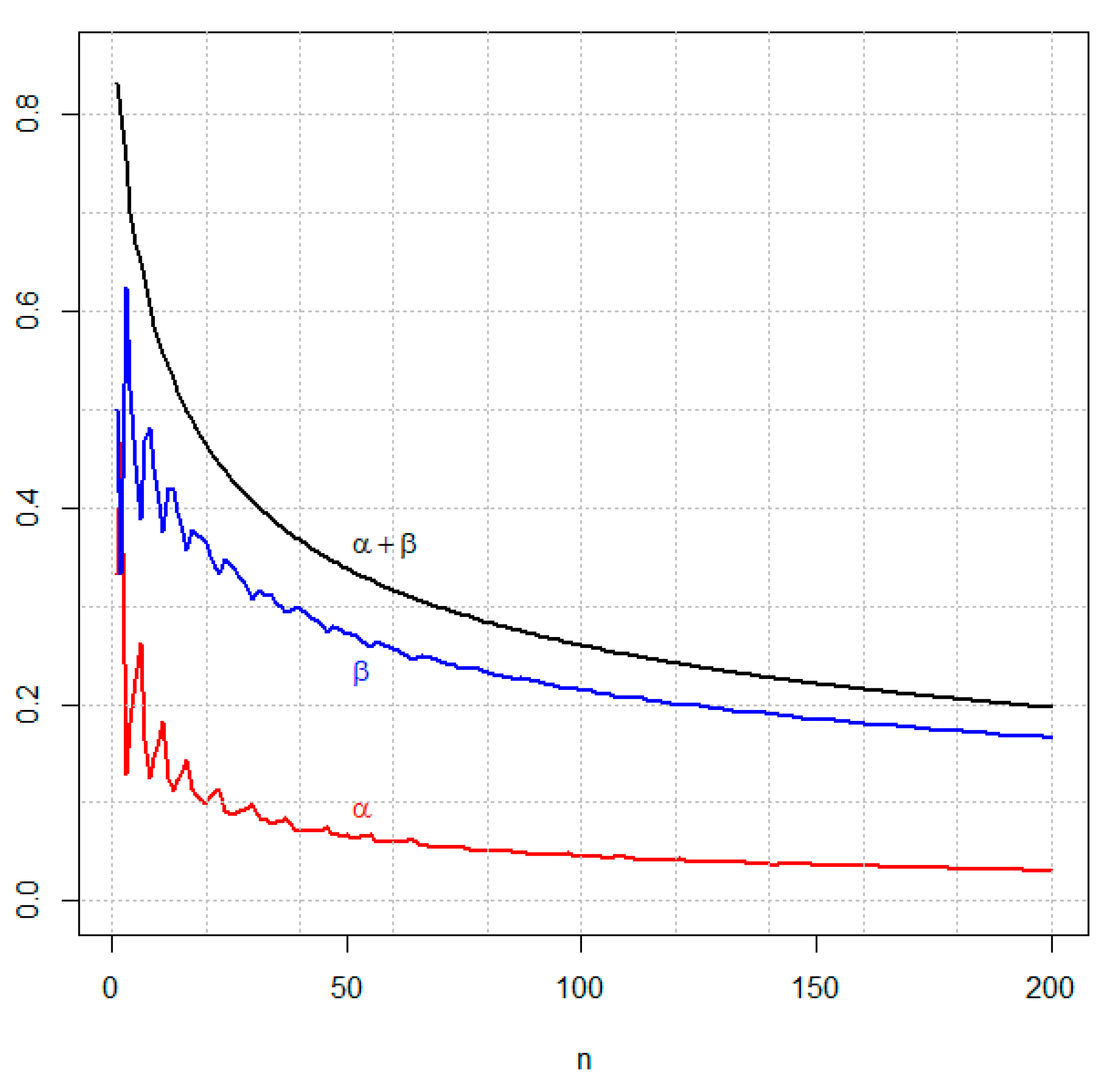
Using the theorem above, compute the optimal averaged error probabilities and use the value of $\alpha \left({\delta }^{*}\right)$ as the adaptive level of significance, which will depend on the loss function, the probability densities, the prior probability$\pi$, and especially on the sample size.

7.

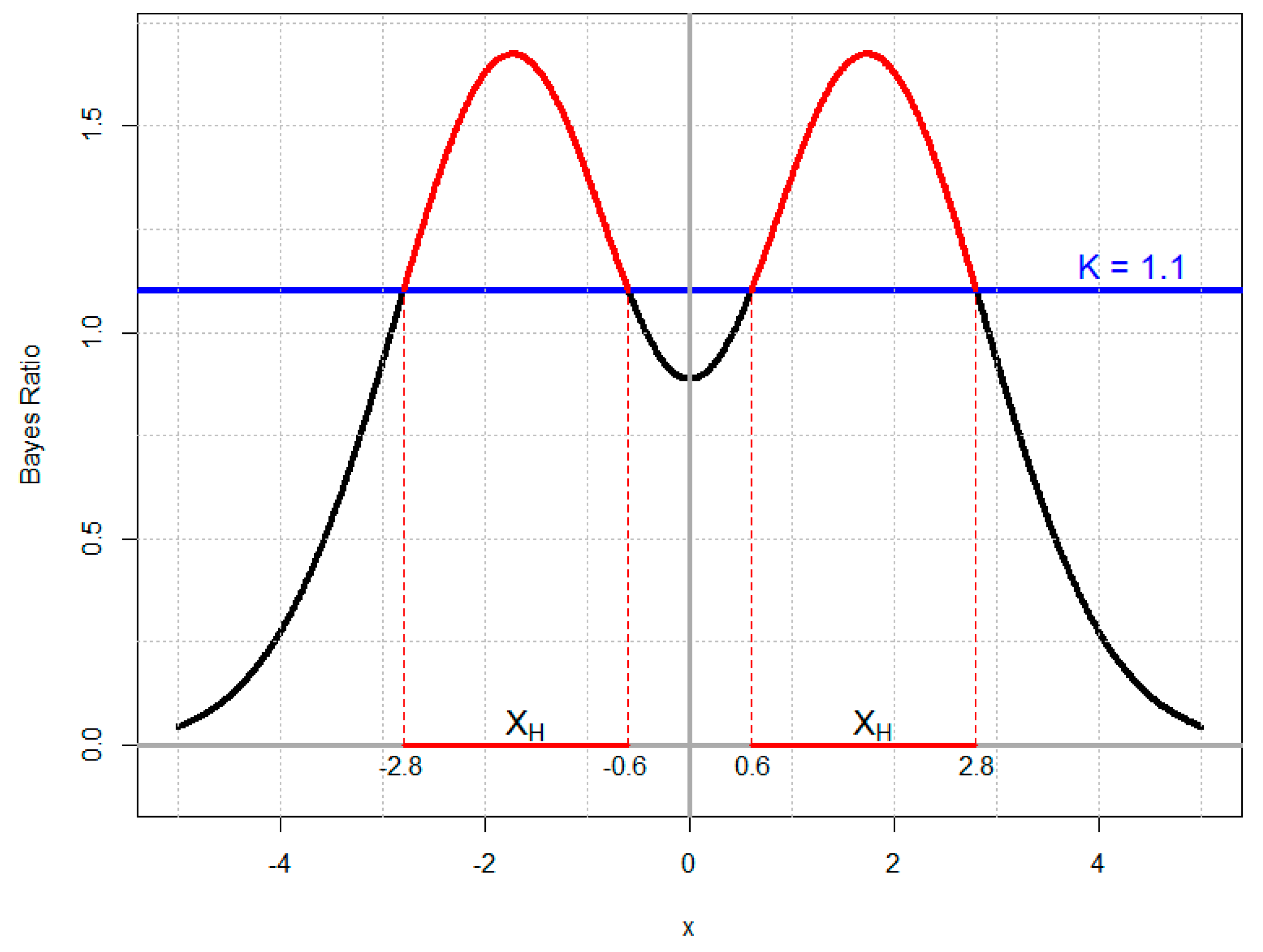
Calculate the significance index, the $P$-value, as follows: if $x_0$ is the observed value of a statistic and $C_0= \left\{x;BF\left(x\right)\le BF\left(x_0\right)\right\}$ is the observed tail under the new ordering, the $P$-value is calculated using the expression $P_0={{\displaystyle \int }}_{C_0}{f}_H\left(x\right)dx$. Clearly, this may be a single or a multiple integral or sum.

8.

Compare the value $P_0$ with the value of $\alpha \left({\delta }^{*}\right).$Reject (do not reject) H if $P_0\begin{array}{c}<\\ (>)\end{array}\alpha \left({\delta }^{*}\right)$. In the case of equality, take either decision without prejudice to optimality.

9.

Finally, if a value of $\alpha \left({\delta }^{*}\right)$ is specified a priori, calculate the sample size needed to make this fixed value as close as possible to optimal according to the generalized Neyman–Pearson Lemma.

We emphasize that it does not matter how the prior over the entire parameter space is chosen. The present work is concerned with how to perform the new hypothesis tests once an overall prior has been chosen.

3. Illustrative Examples

This section introduces four simple examples to illustrate the use of the new $P$-value and how the adaptive significance level varies with sample sizes.

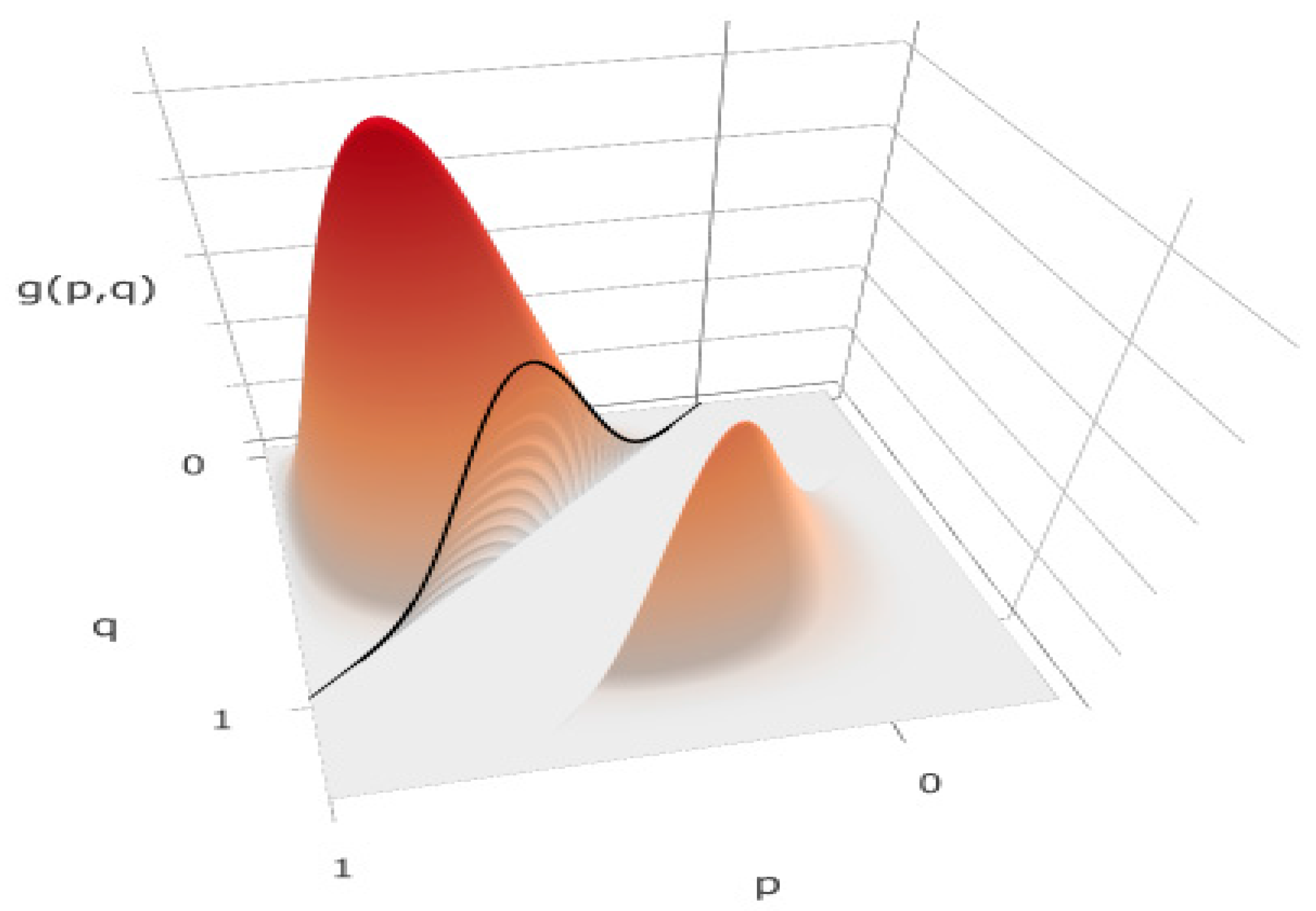
3.1. Example 1—Comparing Two Proportions

A doctor wants to show that the incorporation of a new technology in a treatment can produce better results than the conventional treatment. He plans a clinical trial with two arms, case and control, each with eight patients. The case arm receives the new treatment and the control arm receives the conventional one. Details of a clinical trial of this kind are shown in [33]. The observed results in this example are that only one of the patients in the control arm responded positively, but in the case arm there were four positive outcomes.

The most common classical significance tests result in the following $p$-values: the Pearson χ² $p$-value is 0.106, changed to 0.281 with the Yates continuity correction applied, and Fisher’s exact $p$-value is 0.282. Traditional analysts would conclude that there were no statistically significant differences between the two treatments, using any of the canonical significance levels. Note that these procedures were for testing a sharp hypothesis against a composite alternative: $H:{\theta }_0={\theta }_1\mathrm{and}A:{\theta }_0\ne {\theta }_1,$ comparing the proportion of success of the two treatments. In what follows, we calculate the proposed $P$-value and use the optimal significance level $\alpha \left({\delta }^{*}\right)$ to make the decision of choosing one of the hypotheses.

To be fair in our comparisons, we consider independent uniform (non-informative) prior distributions for${\theta }_0 \mathrm{and} {\theta }_1$. With these suppositions and the likelihoods being binomials with sample sizes n = 8, the predictive probability functions under the two hypotheses are

$$f_H\left(x,y\right)=\frac{\left(\begin{array}{c}8\\ x \end{array}\right)\left(\begin{array}{c}8\\ y\end{array}\right)}{17\left(\begin{array}{c}16\\ x+y\end{array}\right)} \mathrm{and} f_A\left(x,y\right)=\frac{1}{81} \forall \left(x,y\right)\in \left\{0,1,\dots ,8\right\}\times \left\{0,1,\dots ,8\right\}.$$

(11)

The variables $x \mathrm{and} y$represent the possible observed values of the number of positive outcomes in the two arms. Table 1 and Figure 2 present the Bayes factors for all possible results.

Table 1. Bayes factor for all possible results in a clinical trial with arms size of n = 8.

x	y									Sum
	0	1	2	3	4	5	6	7	8
0	4.765	2.382	1.112	0.476	0.183	0.061	0.017	0.003	4e-04	9
1	2.382	2.541	1.906	1.173	0.611	0.267	0.093	0.024	0.003	9
2	1.112	1.906	2.052	1.710	1.166	0.653	0.290	0.093	0.017	9
3	0.476	1.173	1.710	1.866	1.633	1.161	0.653	0.267	0.061	9
4	0.183	0.611	1.166	1.633	1.814	1.633	1.166	0.611	0.183	9
5	0.061	0.267	0.653	1.161	1.633	1.866	1.710	1.173	0.476	9
6	0.017	0.093	0.290	0.653	1.166	1.710	2.052	1.906	1.112	9
7	0.003	0.024	0.093	0.267	0.611	1.173	1.906	2.541	2.382	9
8	4e-04	0.003	0.017	0.061	0.183	0.476	1.112	2.382	4.765	9
Sum	9	9	9	9	9	9	9	9	9	81

Note: Cells with red numbers form the region ${\mathsf{\Psi }}^{*}$ and bold-italic cells are the observed value of the Bayes factor.

Figure 2. Bayes factors of all possible results in a clinical trial with arms size of $n=8$ each.

To obtain the proposed $P$-value, define the set ${\mathsf{\Psi }}_{obs}$ of sample points $\left(x,y\right)$ for which the Bayes factors are smaller than or equal to the Bayes factor of the observed sample point; i.e.,

$${\mathsf{\Psi }}_{obs}=\left\{\left(x,y\right)\in \left\{0,1,\dots ,8\right\}\times \left\{0,1,\dots ,8\right\}:BF\le B{F}_{obs}\right\}.$$

(12)

Thus, the significance index, $P$-value, is the sum of all predictive probabilities (under H) in ${\mathsf{\Psi }}_{obs}$:

$$P-\mathrm{value}={{\displaystyle \sum }}_{\left(x,y\right)\in {\mathsf{\Psi }}_{obs}}{f}_H\left(x,y\right)={{\displaystyle \sum }}_{\left(x,y\right)\in {\mathsf{\Psi }}_{obs}}\frac{\left(\begin{array}{c}8\\ x\end{array}\right)\left(\begin{array}{c}8\\ y\end{array}\right)}{17\left(\begin{array}{c}16\\ x+y\end{array}\right)}.$$

(13)

Recalling the observed result of the clinical trial, $\left(x,y\right)=\left(1,4\right),$the observed Bayes factor is $B{R}_{obs}=0.661$. The italic-bold cells in Table 1 identify the set of possible values of the Bayes factor. Thus, according to Equation (13), the $P$-value is $P=0.0923$.

To obtain the optimal solution we minimize the sum of the error probabilities, $\alpha \left(\delta \right)+\beta \left(\delta \right)$. The two error types are considered to be of the same severity in this example. The optimal solution is the result of comparing the Bayes factor with the constant $K$ as defined in Equation (7) to make the choice according to the extended Neyman–Pearson Lemma. Defining the set of sample space points $\left(x,y\right)$ with Bayes factors smaller than or equal to K, i.e., ${\mathsf{\Psi }}^{*}=\left\{\left(x,y\right)\in \left\{0,1,\dots ,8\right\}\times \left\{0,1,\dots ,8\right\}:BF\le K\right\}$, the optimal Type I and Type II errors are given by

$$\alpha \left({\delta }^{*}\right)={\displaystyle \sum }_{\left(x,y\right)\in {\mathsf{\Psi }}^{*}}{f}_H\left(x,y\right)={\displaystyle \sum }_{\left(x,y\right)\in {\mathsf{\Psi }}^{*}}\frac{\left(\begin{array}{c}8\\ x \end{array}\right)\left(\begin{array}{c}8\\ y \end{array}\right) }{17\left(\begin{array}{c}16\\ x+y\end{array}\right)}$$

(14)

and

$$\beta \left({\delta }^{*}\right)={\displaystyle \sum }_{\left(x,y\right)\notin {\mathsf{\Psi }}^{*}}{f}_A\left(x,y\right)={\displaystyle \sum }_{\left(x,y\right)\notin {\mathsf{\Psi }}^{*}}\frac{1 }{81}.$$

(15)

In this example, we consider the two hypotheses to be equally probable a priori, $\pi =0.5,$ and represent the equal severity of Type-I and Type-II errors by$w_H=w_A=1$, resulting in$K=1$. The set ${\mathsf{\Psi }}^{*}$ was identified by red cells in Table 1. From Equations (14) and (15), we obtain the optimal adaptive level of significance $\alpha \left({\delta }^{*}\right)=0.1245$ and the probability of a Type-II error$\beta \left({\delta }^{*}\right)=0.4815$. The high value of the probability of the second kind of error is expected whenever the sample sizes are small. Contrary to the classical results, the conclusion now is the most intuitive one; the null hypothesis is rejected since $P<\alpha \left({\delta }^{*}\right).$

The physician, owner of the data in Example 1, looking at our analysis, asked about the sample size needed to obtain at most a $10\%$ level of significance for our procedure. The answer could be obtained from the next example, which shows the case of two arms with 20 patients each.

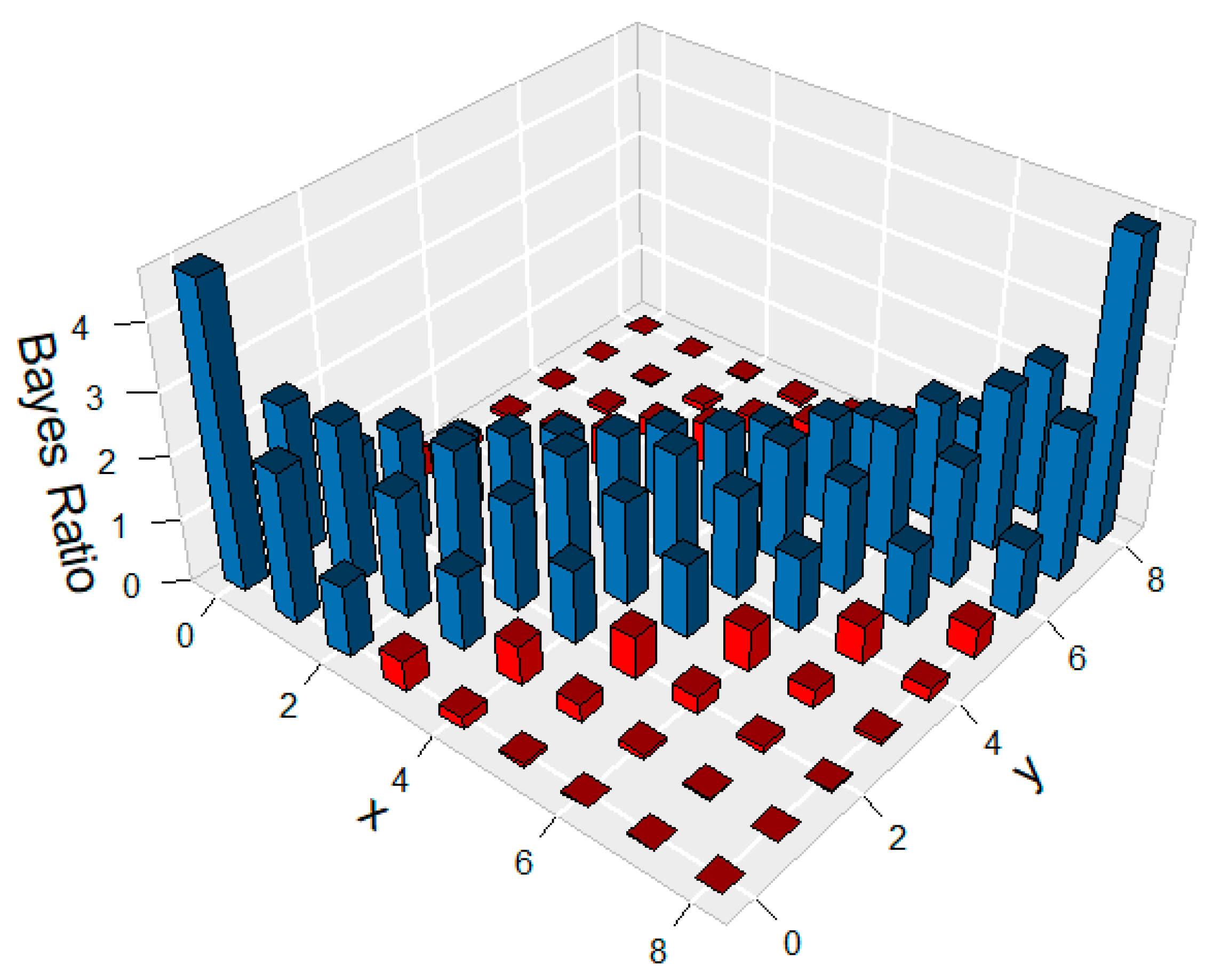
3.2. Example 2—Two Proportions, Varying Sample Sizes

Consider now a clinical trial as in Example 1, but with an arm size of $n=20$. The observed result is$\left(x,y\right)=\left(4,10\right)$. We leave to the reader the simple exercise of repeating the calculations of Example 1 with different samples. Consider independent uniform (non-informative) prior distributions for ${\theta }_0 \mathrm{and} {\theta }_1$ and take the two hypotheses to have equal prior probabilities and the two types of error to have the same relative severity, $\mathsf{\pi }=0.5 \mathrm{and} w_H=w_A=1$. The predictive probability functions under hypotheses $H: {\theta }_0={\theta }_1 \mathrm{and} A:{\theta }_0\ne {\theta }_1$ are

$$f_H\left(x,y\right)=\frac{\left(\begin{array}{c}20\\ x \end{array}\right)\left(\begin{array}{c}20\\ y \end{array}\right) }{41\left(\begin{array}{c}40\\ x+y\end{array}\right)} \mathrm{and} f_A\left(x,y\right)=\frac{1 }{441}\forall \left(x,y\right)\in \left\{0,1,\dots ,20\right\}\times \left\{0,1,\dots ,20\right\}$$

(16)

and the observed Bayes factor is $B{F}_{obs}=0.415$, which leads to the following results: significance index $P=0.02901$; optimal adaptive level of significance $\alpha \left({\delta }^{*}\right)=0.0995$; and the probability of a Type-II error $\beta \left({\delta }^{*}\right)=0.3651$. The classical χ² $p$-value is$p = 0.0467$, indicating rejection of the null hypothesis at the canonical $5\%$level of significance. This agrees with our decision of rejecting the null hypothesis since again$P<\alpha \left({\delta }^{*}\right)$. It is interesting to see the relative distance between the index and the level of significance. For the χ² test, we have $1- \frac{0.0467}{0.05}=0.07$ and the adaptive case obtains $1- \frac{0.029 }{0.0995}=0.71$.

Figure 3 presents the optimal adaptive level of significance and the Type-II error by sample size. As expected, the probabilities of both kinds of errors decrease when the sample size increases.

Figure 3. Type-I and Type-II error probabilities as functions of the sample size n in each arm.

The response to the question about the sample size needed to obtain a significance level of at most $10\%$ is $n = 20$ in each arm. For a level of at most$5\%$, we need a sample size of $n=90$in each arm.

Optimal adaptive significance levels and Type-II error probabilities for different arm sizes, $n_1$ and $n_2$ are presented in Table 2. With a fixed total sample size, an unbalanced sample can have larger (both Type-I and Type-II) errors than a balanced sample. The greater the imbalance of the sample, the greater the averaged error probabilities is. For example, the error probabilities of an unbalanced sample with $n_1=60$ and $n_2$ $=10$ is larger than a balanced sample with n₁ = n₂ = 20 (Table 2), despite the unbalanced sample having a total size of $70$ and the balanced sample just 40.

Table 2. Optimal levels of significance ($\alpha$ ) and Type-II error probabilities ($\beta )$ for two proportions: Two independent binomial likelihoods and various sample sizes.

${\mathit{n}}_1$	${\mathit{n}}_2$	$\mathit{\alpha }$	$\mathit{\beta }$	${\mathit{n}}_1$	${\mathit{n}}_2$	$\mathit{\alpha }$	$\mathit{\beta }$	${\mathit{n}}_1$	${\mathit{n}}_2$	$\mathit{\alpha }$	$\mathit{\beta }$	${\mathit{n}}_1$	${\mathit{n}}_2$	$\mathit{\alpha }$	$\mathit{\beta }$
10	10	0.1639	0.4050	50	50	0.0667	0.2718	80	10	0.1130	0.3648	90	70	0.0529	0.2323
20	10	0.1318	0.3939	60	10	0.1097	0.3741	80	20	0.0834	0.3122	90	80	0.0493	0.2281
20	20	0.0995	0.3651	60	20	0.0860	0.3193	80	30	0.0704	0.2847	90	90	0.0468	0.2240
30	10	0.1159	0.3900	60	30	0.0765	0.2903	80	40	0.0634	0.2671	100	10	0.1111	0.3627
30	20	0.1045	0.3333	60	40	0.0689	0.2747	80	50	0.0603	0.2530	100	20	0.0818	0.3079
30	30	0.0997	0.3070	60	50	0.0626	0.2652	80	60	0.0553	0.2455	100	30	0.0684	0.2795
40	10	0.1250	0.3703	60	60	0.0591	0.2572	80	70	0.0531	0.2380	100	40	0.0617	0.2601
40	20	0.0868	0.3357	70	10	0.1130	0.3675	80	80	0.0508	0.2327	100	50	0.0559	0.2479
40	30	0.0850	0.3029	70	20	0.0865	0.3132	90	10	0.1131	0.3626	100	60	0.0538	0.2368
40	40	0.0706	0.2968	70	30	0.0727	0.2876	90	20	0.0810	0.3114	100	70	0.0512	0.2291
50	10	0.1126	0.3761	70	40	0.0645	0.2717	90	30	0.0707	0.2804	100	80	0.0483	0.2238
50	20	0.0883	0.3240	70	50	0.0603	0.2593	90	40	0.0648	0.2608	100	90	0.0467	0.2188
50	30	0.0767	0.2992	70	60	0.0575	0.2501	90	50	0.0575	0.2506	100	100	0.0449	0.2150
50	40	0.0718	0.2817	70	70	0.0539	0.2446	90	60	0.0550	0.2401

Pericchi and Pereira [6] present a closed asymptotic formula that relates sample size and significance level in the simple case of testing $H: \theta ={\theta }_0 \mathrm{vs}. A:\theta \ne {\theta }_0,$ in a binomial with parameters$\theta \mathrm{and} n$. A natural future project is to find this type of relation in other complex statistical problems such as the one presented in the above examples.

The following example is an attempt to show that our $P$-value should not violate the likelihood principle. Recall that violation of this principle has produced some of the Bayesian community’s main criticisms of the classical p-values.

3.3. Example 3—Test for One Proportion and the Likelihood Principle

A common example in which the likelihood principle can be violated is the case of binomials compared to negative binomials. For the same values of x, the number of successes in n independent Bernoulli trials, the two distributions produce different $p$-values that can lead to different decisions if compared with the same level of significance. The present example shows that the new test introduced here will produce identical decisions if the observed sample size and the number of successes are the same. The proof that this is the case in general for the new tests is presented as Appendix A to this article. The reason the decisions end up being the same for different models is that, although the $P$-values for the different models are different from each other, they are compared to different significance levels. The decision about the null hypothesis ends up being the same, so there is no violation of the likelihood principle. Changing the notation, let the sample vector be composed of the number of success and the number of failures, $\left(x,y\right),$ and the corresponding vector of probabilities be $({\theta }_0,{\theta }_1) \mathrm{with} {\theta }_0=1-{\theta }_1.$Take $H: {\theta }_1=0.5 \mathrm{and} A:{\theta }_1\ne 0.5$as the hypotheses to be tested. Taking a uniform (non-informative) prior distribution for ${\theta }_1$ and taking the two hypotheses to be equally probable a priori and the two types of error to have equal relative severity, $\mathsf{\pi }=0.5$ $\mathrm{with} w_H=w_A=1$, the predictive densities needed for the significance tests are as follows:

• for a (positive) binomial,

  $$f_H\left(x\right)=\left(\begin{array}{c}x+y\\ x\end{array}\right){\left(\frac{1}{ 2 }\right)}^{x+y} \mathrm{and} f_A\left(x\right)={\left(x+y+1\right)}^{-1}$$

  (17)
• for a negative binomial,

  $$f_H\left(x\right)=\left(\begin{array}{c}x+y-1\\ x\end{array}\right){\left(\frac{1}{ 2 }\right)}^{x+y} \mathrm{and} f_A\left(x\right)=y{\left[\left(x+y\right)\left(x+y+1\right)\right]}^{-1}.$$

  (18)

Clearly, the Bayes factors, as defined by Equation (9), are equal for the two models, and since using the lemma will lead to comparing them to the same constant, the decisions about the null hypothesis end up being the same. Note that both the $P$-values and the significance levels are different for the two models. For instance, if we consider the observations $\left(x,y\right)=\left(3,10\right) \mathrm{and} \left(x,y\right)=\left(10,3\right)$for a positive binomial, we obtain the same results for both samples; $\alpha =0.09, \beta =0.43, \mathrm{and} P=0.02$. For the negative binomial, the two observed points will produce different significance levels and probabilities of both kinds of errors. For the first (second) sample, one stops observing whenever the number of successes reaches 3 Equation (11). For the first result, we have$\alpha =0.18$, $\beta =0.4$and$P=0.0$; for the second$, \alpha =0.12, \beta =0.33, \mathrm{and} P=0.01$. Therefore, the decisions based on positive binomials are the same as the ones based on negative binomials for the same$\left(x,y\right)$.

Table 3 presents the predictive densities under several kinds of hypotheses for one proportion. For all kinds of hypotheses, positive and negative binomial models, for the same $\left(x,y\right)$, produce equal Bayes factors.

Table 3. Predictive densities under several hypotheses for one proportion.

Hypotheses	Predictive Densities under H 1
H: $\mathit{\theta }$ = $\mathit{\theta }$0	$\mathit{C}\left(\mathit{x},\mathit{y}\right){\mathit{\theta }}_{\mathbf{0}}^{\mathit{x}}{\left(\mathbf{1}-{\mathit{\theta }}_{\mathbf{0}}\right)}^{\mathit{y}}$
H: $\mathit{\theta }\ne \mathit{\theta }$0	$\mathit{C}\left(\mathit{x},\mathit{y}\right)\frac{\mathit{B}\left(\mathit{U},\mathit{V}\right)}{\mathit{B}\left(\mathit{u},\mathit{v}\right)}$
H: $\mathit{\theta }$ ≤$\mathit{\theta }$0	$\mathit{C}\left(\mathit{x},\mathit{y}\right)\frac{\mathit{B}\left({\mathit{\theta }}_{\mathbf{0}};\mathit{U},\mathit{V}\right)}{\mathit{B}\left({\mathit{\theta }}_{\mathbf{0}};\mathit{u},\mathit{v}\right)}$
H: $\mathit{\theta }$ > $\mathit{\theta }$0	$\mathit{C}\left(\mathit{x},\mathit{y}\right)\frac{\mathit{B}\left(\mathit{U},\mathit{V}\right)-\mathit{B}\left({\mathit{\theta }}_{\mathbf{0}};\mathit{U},\mathit{V}\right)}{\mathit{B}\left(\mathit{u},\mathit{v}\right)-\mathit{B}\left({\mathit{\theta }}_{\mathbf{0}};\mathit{u},\mathit{v}\right)}$
H: $\mathit{\theta }$1 ≤ $\mathit{\theta }$ ≤ $\mathit{\theta }$2	$\mathit{C}\left(\mathit{x},\mathit{y}\right)\frac{\mathit{B}\left({\mathit{\theta }}_{\mathbf{2}};\mathit{U},\mathit{V}\right)-\mathit{B}\left({\mathit{\theta }}_{\mathbf{1}};\mathit{U},\mathit{V}\right)}{\mathit{B}\left({\mathit{\theta }}_{\mathbf{2}};\mathit{u},\mathit{v}\right)-\mathit{B}\left({\mathit{\theta }}_{\mathbf{1}};\mathit{u},\mathit{v}\right)}$
H: ($\mathit{\theta }$ < $\mathit{\theta }$1)∪($\mathit{\theta }$ > $\mathit{\theta }$2)	$\mathit{C}\left(\mathit{x},\mathit{y}\right)\frac{\mathit{B}\left(\mathit{U},\mathit{V}\right)-\mathit{B}\left({\mathit{\theta }}_{\mathbf{2}};\mathit{U},\mathit{V}\right)+\mathit{B}\left({\mathit{\theta }}_{\mathbf{1}};\mathit{U},\mathit{V}\right)}{\mathit{B}\left(\mathit{u},\mathit{v}\right)-\mathit{B}\left({\mathit{\theta }}_{\mathbf{2}};\mathit{u},\mathit{v}\right)+\mathit{B}\left({\mathit{\theta }}_{\mathbf{1}};\mathit{u},\mathit{v}\right)}$
H: ($\mathit{\theta }$1 ≤ $\mathit{\theta }$ ≤ $\mathit{\theta }$2)∪($\mathit{\theta }$3 ≤ $\mathit{\theta }$ ≤ $\mathit{\theta }$4)	$\mathit{C}\left(\mathit{x},\mathit{y}\right)\frac{\mathit{B}\left({\mathit{\theta }}_{\mathbf{2}};\mathit{U},\mathit{V}\right)-\mathit{B}\left({\mathit{\theta }}_{\mathbf{1}};\mathit{U},\mathit{V}\right)+\mathit{B}\left({\mathit{\theta }}_{\mathbf{4}};\mathit{U},\mathit{V}\right)-\mathit{B}\left({\mathit{\theta }}_{\mathbf{3}};\mathit{U},\mathit{V}\right)}{\mathit{B}\left({\mathit{\theta }}_{\mathbf{2}};\mathit{u},\mathit{v}\right)-\mathit{B}\left({\mathit{\theta }}_{\mathbf{1}};\mathit{u},\mathit{v}\right)+\mathit{B}\left({\mathit{\theta }}_{\mathbf{4}};\mathit{u},\mathit{v}\right)-\mathit{B}\left({\mathit{\theta }}_{\mathbf{3}};\mathit{u},\mathit{v}\right)}$
H: ($\mathit{\theta }$ < $\mathit{\theta }$1)∪$(\mathit{\theta }$2 < $\mathit{\theta }$ < $\mathit{\theta }$3)∪($\mathit{\theta }$ > $\mathit{\theta }$4)	$\mathit{C}\left(\mathit{x},\mathit{y}\right)\frac{\mathit{B}\left(\mathit{U},\mathit{V}\right)-\mathit{B}\left({\mathit{\theta }}_{\mathbf{2}};\mathit{U},\mathit{V}\right)+\mathit{B}\left({\mathit{\theta }}_{\mathbf{1}};\mathit{U},\mathit{V}\right)-\mathit{B}\left({\mathit{\theta }}_{\mathbf{4}};\mathit{U},\mathit{V}\right)+\mathit{B}\left({\mathit{\theta }}_{\mathbf{3}};\mathit{U},\mathit{V}\right)}{\mathit{B}\left(\mathit{u},\mathit{v}\right)-\mathit{B}\left({\mathit{\theta }}_{\mathbf{2}};\mathit{u},\mathit{v}\right)+\mathit{B}\left({\mathit{\theta }}_{\mathbf{1}};\mathit{u},\mathit{v}\right)-\mathit{B}\left({\mathit{\theta }}_{\mathbf{4}};\mathit{u},\mathit{v}\right)+\mathit{B}\left({\mathit{\theta }}_{\mathbf{3}};\mathit{u},\mathit{v}\right)}$

¹ Prior distribution for $\theta$: $\theta ~Beta\left(u,v\right)$; $U=u+x$; $V=v+y$; $C\left(x,y\right)=\left(\begin{array}{c}x+y\\ x\end{array}\right)$ for positive binomial or $C\left(x,y\right)=\left(\begin{array}{c}x+y-1\\ x\end{array}\right)$ for negative binomial; $B\left(r,s\right)={{\displaystyle \int }}_0^1{z}^{r-1}{\left(1-z\right)}^{s-1}dz$ is the beta functions; and $B\left(p;r,s\right)={{\displaystyle \int }}_0^p{z}^{r-1}{\left(1-z\right)}^{s-1}dz$ is the incomplete beta function.

3.4. Example 4

This is an example used by Pereira and Wechsler [15], showing that the critical region is not always the tails of the null distribution; it can be a union of disjoint intervals. In such cases, it can be impossible to calculate a classical $p$-value, but the ordering of the entire sample space by Bayes factors allows for an unambiguous definition and calculation of the new index, a $P$-value.

Let x be a normal random variable with zero mean and unknown variance${\sigma }^2$. The hypotheses are $H: {\sigma }^2=2 \mathrm{vs}.A: {\sigma }^2\ne 2$. A ${\mathit{\chi }}_1^2$ (chi-squared distribution with one degree of freedom) is taken as a prior density for${\sigma }^2$. After an integration exercise, we can establish the predictive densities for our significance test as

$$f_A\left(x\right)={\left\{\mathsf{\pi }\left(1+x^2\right)\right\}}^{-1}\hspace{1em}\mathrm{and}\hspace{1em}{f}_H\left(x\right)={\left(2\sqrt{\mathsf{\pi }}\right)}^{-1}\exp \left(-\frac{x^2}{4}\right).$$

(19)

These are, respectively, a Cauchy density and a normal density with zero mean and variance 2. Figure 4 shows the Bayes factor for all sample points, using the constant 1.1 as a cutoff for the decision about the null hypothesis. The sample points that do not favor the null hypothesis are a central region together with the heavy tails of the Cauchy density. The set that favors $H$ does not include the central region:

$${\mathit{X}}_H=\left\{x|x\in \left(-2.8;-0.6\right){{\displaystyle \cup }}^{}\left(0.6;2.8\right)\right\}$$

(20)

Figure 4. Bayes factor for $N\left(0;2\right)$ vs. Cauchy.

The set favoring the alternate hypothesis $A$ includes the interval $\left(-0.6;0.6\right),$ a considerable central region.

4. Final Remarks

It is worth noting that there are multiple ways to understand our new test, and we would like to present a specific vision. Consider a statistical model, with a family of probability functions indexed by$\theta ,$ denoted by $f\left(x|\theta \right),$ with all necessary conditions imposed for all relevant mathematical objects to be well-defined. If λ is a function of$\theta$, one can simply write$f(x|\theta )=f(x|\theta ,\lambda )$, because the sub-σ-algebra defined by the new parameter λ is contained in the one defined by the original parameter$\theta$. Given a prior density $g\left(\theta \right)$ for the original parameter $\theta ,$

$$f\left(x|\lambda \right)=E_{\theta }\left\{L\right(\lambda ,\theta |x)\}=E_{\theta }\left\{g\left(\theta |\lambda \right)f\left(x|\theta ,\lambda \right)\right\}.$$

(21)

If the new parameter λ is a binary function (produces only values 0 and 1), then the two predictive probability functions are $f_0\left(x\right)=f\left(x|\lambda =0\right) \mathrm{and} f_1\left(x\right)=f\left(x|\lambda =1\right)$. These functions are averages, weighted by $g\left(\theta |\lambda \right),$ of the likelihood function. The original parameter has been removed as a “nuisance”, leaving only the new parameter representing the decision. Because the new parameter is binary, hypotheses involving it are simple-versus-simple, so the generalized Neyman–Pearson Lemma applies. Our procedure can be seen as elimination of a nuisance parameter for the application of optimization. We refer to Basu [34] for elimination of nuisance parameters when the parameter spaces are variation dependent.

For decades, and increasingly in recent years, users of statistics have been questioning the logic of using the canonical significance levels, or indeed, any fixed significance level, for hypothesis testing. We believe that there are no formal reasons for using the established numbers, and that there are in fact good reasons not to fix significance levels a priori. We use the natural logic of optimization to define an adaptive significance level, that is, one that depends on the sample size. Our test using the new index ($P$-value) and the adaptive significance level is compatible with the likelihood principle, as proved in the Appendix A of the present article.

There is still much work to be done, testing different kinds of hypotheses in the parameter spaces of different models, including multivariate problems. We are not aware of any complex model that prevents the use of the hypothesis tests discussed in the present paper. It is hoped that the similarity of the apparatus of the new tests to that of existing Neyman–Pearson tests, plus favorable characteristics of the new tests, will make the new testing procedure useful and popular among investigators in the many fields in which statistical hypothesis testing can be useful.

There is certainly a one-to-one relation between$P$and$BF$! Hence, after a cut-off for $P$ is defined automatically, we have a corresponding cut-off for $BF$ and there is then a one-to-one correspondence of the pair of error type probabilities between the two methods. Those who prefer to use Bayes factors directly can certainly do so, but they can also advantage of the cut-off provided by our method.

References

- Johnson, V.E. Revised standards for statistical evidence. Proc. Natl. Acad. Sci. USA 2013, 110, 19313–191317. [Google Scholar] [CrossRef] [PubMed]
- Gaudart, J.; Huiart, L.; Milligan, P.J.; Thiebaut, R.; Giorgi, R. Reproducibility issues in science, is P value really the only answer? Proc. Natl. Acad. Sci. USA 2014, 111, E1934. [Google Scholar] [CrossRef] [PubMed]
- Gelman, A.; Robert, C.P. Revised evidence for statistical standards. Proc. Natl. Acad. Sci. USA 2014, 111, E1933. [Google Scholar] [CrossRef] [PubMed]
- Pericchi, L.; Pereira, C.A.B.; Pérez, M.E. Adaptive revised evidence for statistical standards. Proc. Natl. Acad. Sci. USA 2014, 111, E1935. [Google Scholar] [CrossRef] [PubMed]
- Wasserstein, R.L.; Lazar, N.A. The ASA’s statement on p-values: Context, process, and purpose. Am. Stat. 2016, 70, 129–133. [Google Scholar] [CrossRef]
- Pericchi, L.R.; Pereira, C.A.B. Adaptive significance levels using optimal decision rules: Balancing by weighting the error probabilities. Braz. J. Probab. Stat. 2016, 30, 70–90. [Google Scholar]
- Benjamin, D.; Berger, J.; Johannesson, M.; Nosek, B.A.; Wagenmakers, E.-J.; Berk, R.; Bollen, K.A.; Brembs, B.; Brown, L.; Camerer, C.; et al. Redefine statistical significance. Nat. Hum. Behav. 2017. [Google Scholar] [CrossRef]
- Nature News. Big Names in Statistics Want to Shake up Much-Maligned P Value. Available online: https://www.nature.com/articles/d41586-017-02190-5?WT.mc_id=TWT_NatureNews&sf101140733=1 (accessed on 28 August 2017).
- Pereira, C.A.B.; Stern, J.M. Evidence and credibility: A full Bayesian test of precise hypotheses. Entropy 1999, 1, 104–115. [Google Scholar]
- Madruga, M.R.; Pereira, C.A.B.; Stern, J.M. Bayesian evidence test for precise hypotheses. J. Stat. Plan. Inference 2002, 117, 185–198. [Google Scholar] [CrossRef]
- Pereira, C.A.B.; Stern, J.M.; Wechsler, S. Can a significance test be genuinely Bayesian? Bayesian Anal. 2008, 3, 79–100. [Google Scholar] [CrossRef]
- Stern, J.M.; Pereira, C.A.B. Bayesian epistemic values: Focus on surprise, measure probability! Log. J. IGPL 2013, 22, 236–254. [Google Scholar] [CrossRef]
- Chakrabarty, D. A New Bayesian Test to Test for the Intractability-Countering Hypothesis. J. Am. Stat. Assoc. 2017, 112, 561–577. [Google Scholar] [CrossRef]
- Diniz, M.A.; Pereira, C.A.B.; Polpo, A.; Stern, J.M.; Wechsler, S. Relationship between Bayesian and frequentist significance indices. Int. J. Uncertain. Quantif. 2012, 2, 161–172. [Google Scholar] [CrossRef]
- Pereira, C.A.B.; Wechsler, S. On the concept of p-value. Braz. J. Probab. Stat. 1993, 7, 159–177. [Google Scholar]
- Pereira, C.A.B. Testing Hypotheses of Different Dimensions: Bayesian View and Classical Interpretation. Professor Thesis, Institute Mathematics & Statistics, USP, Sao Paulo, Brazil, 1985. (In Portuguese). [Google Scholar]
- Irony, T.Z.; Pereira, C.A.B. Bayesian hypothesis test: Using surface integrals to distribute prior information among the hypotheses. Resenhas 1995, 2, 27–46. [Google Scholar]
- Montoya-Delgado, L.E.; Irony, T.Z.; Pereira, C.A.B.; Whittle, M.R. An unconditional exact test for the Hardy-Weinberg equilibrium law: Sample space ordering using the Bayes factor. Genetics 2001, 158, 875–883. [Google Scholar] [PubMed]
- DeGroot, M.H. Probability and Statistics; Addison-Wesley: Boston, MA, USA, 1986. [Google Scholar]
- Dawid, A.P.; Lauritzen, S.L. Compatible Prior Distributions. In Bayesian Methods with Applications to Science Policy and Official Statistics; Monographs of Official Statistics; EUROSTAT: Luxembourg, 2001; pp. 109–118. [Google Scholar]
- Dickey, J.M. The weighted likelihood ratio, linear hypotheses on normal location parameters. Ann. Math. Stat. 1971, 42, 204–223. [Google Scholar] [CrossRef]
- Cox, D.R. The role of significance tests (with discussions). Scand. J. Stat. 1977, 4, 49–70. [Google Scholar]
- Cox, D.R. Principles of Statistical Inference; Cambridge University Press: New York, NY, USA, 2006. [Google Scholar]
- Evans, M. Measuring statistical evidence using relative belief. Comput. Struct. Biotechnol. J. 2016, 14, 91–96. [Google Scholar] [CrossRef] [PubMed]
- Lindley, D.V. A Statistical Paradox. Biometrika 1957, 44, 187–192. [Google Scholar] [CrossRef]
- Bartlett, M.S. A comment on D.V. Lindley’s statistical paradox. Biometrika 1957, 44, 533–534. [Google Scholar] [CrossRef]
- Cornfield, J. Sequential trials, sequential analysis and the likelihood principle. Am. Stat. 1966, 20, 18–23. [Google Scholar]
- Neyman, J.; Pearson, E.S. On the problem of the most efficient tests of statistical hypotheses. Philos. Trans. R. Soc. Lond. Ser. A Contain. Pap. A Math. Phys. Charact. 1933, 231, 289–337. [Google Scholar] [CrossRef]
- García-Donato, G.; Chen, M.-H. Calibrating Bayes factor under prior predictive distributions. Stat. Sin. 2005, 15, 359–380. [Google Scholar]
- Jeffreys, H. The Theory of Probability; The Clarendon Press: Oxford, UK, 1935. [Google Scholar]
- Gu, X.; Hoijtink, H.; Mulder, J. Error probabilities in default Bayesian hypothesis testing. J. Math. Psychol. 2016, 72, 140–143. [Google Scholar] [CrossRef]
- Kass, R.E.; Raftery, A.E. Bayes Factors. JASA 1995, 90, 773–795. [Google Scholar] [CrossRef]
- Lopes, A.C.; Greenberg, B.D.; Canteras, M.M.; Batistuzzo, M.C.; Hoexter, M.Q.; Gentil, A.F.; Pereira, C.A.B.; Joaquim, M.A.; de Mathis, M.E.; D’Alcante, C.C.; et al. Gamma Ventral Capsulotomy for Obsessive-Compulsive Disorder: A Randomized Clinical Trial. JAMA Psych. 2014, 71, 1066–1076. [Google Scholar] [CrossRef] [PubMed]
- Basu, D. On the elimination of nuisance parameters. JASA 1977, 72, 355–366. [Google Scholar] [CrossRef]
© 2017 by the authors. Licensee MDPI, Basel, Switzerland. This article is an open access article distributed under the terms and conditions of the Creative Commons Attribution (CC BY) license (http://creativecommons.org/licenses/by/4.0/).