Article

Combined Forecasting of Rainfall Based on Fuzzy Clustering and Cross Entropy

1
Beijing Key Laboratory of Energy Safety and Clean Utilization, North China Electric Power University, Renewable Energy Institute, Beijing 102206, China
2
State Key Laboratory of New Energy Power System, North China Electric Power University, Beijing 102206, China
3
Key Laboratory of Water Cycle and Related Land Surface Process, Institute of Geographic Sciences and Natural Resources Research, Chinese Academy of Sciences, Beijing 100101, China
4
University of Chinese Academy of Sciences, Beijing 100049, China
*
Author to whom correspondence should be addressed.
Entropy 2017, 19(12), 694; https://doi.org/10.3390/e19120694
Submission received: 31 August 2017 / Revised: 5 December 2017 / Accepted: 14 December 2017 / Published: 19 December 2017
(This article belongs to the Special Issue Entropy Applications in Environmental and Water Engineering)

Abstract

:
Rainfall is an essential index to measure drought, and it is dependent upon various parameters including geographical environment, air temperature and pressure. The nonlinear nature of climatic variables leads to problems such as poor accuracy and instability in traditional forecasting methods. In this paper, the combined forecasting method based on data mining technology and cross entropy is proposed to forecast the rainfall with full consideration of the time-effectiveness of historical data. In view of the flaws of the fuzzy clustering method which is easy to fall into local optimal solution and low speed of operation, the ant colony algorithm is adopted to overcome these shortcomings and, as a result, refine the model. The method for determining weights is also improved by using the cross entropy. Besides, the forecast is conducted by analyzing the weighted average rainfall based on Thiessen polygon in the Beijing–Tianjin–Hebei region. Since the predictive errors are calculated, the results show that improved ant colony fuzzy clustering can effectively select historical data and enhance the accuracy of prediction so that the damage caused by extreme weather events like droughts and floods can be greatly lessened and even kept at bay.

1. Introduction

Rainfall forecasts play an important role in agricultural production, urban industry and life. The accurate prediction of rainfall has significant economic and social value. It can provide data support for the relevant departments and help detect droughts and floods and reduce the degree of harm. However, affected by complex factors such as geographical environment, ocean currents, air pressure, temperature, etc. [1], rainfall exhibits strong randomness and nonlinear characteristics that often hamper the forecast of rainfall.
The rainfall prediction methods discussed in this paper are based on mathematical models and algorithms, through the full mining of historical data to establish the forecasting model. At present, a variety of approaches have been applied to predict rainfall at home and abroad and basically they can be classified into five categories: (1) Numerical prediction model. This model is based on the physical model of process. Its advantage lies in the fast speed and easy procedure, but due to the impact of the memory required in can only reasonably be used for monthly forecasts and for longer periods (such as an annual forecast) is difficult to use [2,3]; (2) Time series model exponential smoothing. The moving average method and Autoregressive Integrated Moving Average Model (ARIMA) [4] belong to this type; they can better describe the linear change process yet sometimes they are not suitable for non-stationary random processes; (3) Probabilistic simulation methods. These include the grey model (GM) [5] and Monte Carlo method [6]. The prediction of exponential trends is more accurate with the grey model, but it is only suitable for short and medium term forecasting and the longer the forecast lasts, the larger the errors that may occur. The Monte Carlo method is characterized by describing the random process, but the support of data is also required; (4) Artificial intelligence methods such as radical basis function (RBF), genetic algorithm (GA), wavelet analysis (WA) [7,8,9,10], can better simulate nonlinear processes with higher prediction accuracy, but may fail due to issues like local optima, overlearning and weak generalization ability; (5) in addition there are some other methods, like Numerical Weather Prediction (NWP) [11,12], R/S analysis [13], trend analysis [14], etc. that can predict rainfall from different angles, but two problems should not be ignored: first, in the long-term forecast, rainfall is a random process hence any single forecasting method cannot ensure the stability during the process of prediction. Additionally, serious errors may occur at certain times resulting in the failure of prediction. Second, obtaining useful information with a single method is one-sided, and overlooks different factors from all perspectives.
For the prediction of rainfall, a large amount of historical data is necessary to ensure the accuracy of the forecast. Nonetheless, historical data inevitably contains some errors or abnormal information and this affects the accuracy of the forecast because rainfall is associated with many factors such as temperature, climate, and human activities. Therefore, the forecast method based on fuzzy clustering prediction method has been applied in recent years [15,16]. However, the traditional fuzzy clustering algorithm approach easily falls into local optimal solutions, and it is difficult to deal with a large number of high-dimensional data from a time performance point of view [17]. In this paper, the ant colony algorithm is proposed to improve the fuzzy clustering. With this method, the reliability and computational efficiency of data filtering and processing are greatly increased.
Bates and Granger established the combined forecasting method based on weights in 1969 [18]. The approach combines the different methods and the features of data to improve the accuracy of forecasting and reduce the risk of failure. The combined forecasting method has been widely used in various fields, including electric power load forecasting, economics, logistics, etc., and facts have proven how effective the method is [19,20,21,22]. Nonetheless, as a simple combination of several single methods, the previous method neglects the bias of the selection of a single method. Furthermore, there is no detailed analysis of the time characteristics of historical data. At present, some scholars are paying attention to combined forecasting in the field of rainfall forecasting [23,24,25]. In Cui’s study [23], the wavelet analysis method aims to determine the weight reconstruction of the rainfall forecast, yet the time distribution of historical data is not considered. In Xiong’s study [24] and Lu’s study [25], real-time river flow or flood forecasting methods have been studied, but they are not suitable for medium and long-term prediction.
The concept of entropy propounded by the German physicist Clausius in 1877 is a function of the state of the system, but the reference value and the variation of entropy are often analyzed and compared. Cross Entropy (CE) is a kind of entropy that reflects the similarity between variables from the perspective of probability. The application of entropy theory in hydrology mainly include the derivation of the distributions and estimation of the corresponding parameters for hydrometeorological variables [26,27,28], dependence analysis [29] and runoff forecasting [30,31,32,33,34]. The cross entropy is introduced into the combination forecasting by Li et al. [24,25]. Their research put forward a new method of determining weight, which improves the stability of the prediction results. However, the probability density function [24] is not suitable for the prediction of radial flow. The wind power load forecasting method based on normal distribution is proposed by Chen et al. [25]. The time characteristic of historical data is not considered in this method and the solution is too complex to be implemented.
The key of the prediction method based on historical data is not only a prediction model, but also a validity of historical data. And that is the category of data mining. The choice of historical data is fundamentally a clustering process, so clustering method is very important. In terms of the weaknesses of the fuzzy clustering method, the ant colony algorithm attempts to improve the model. Meanwhile, the method for determining weights is also improved by using the cross entropy (CE).

2. Improved Fuzzy Clustering Model
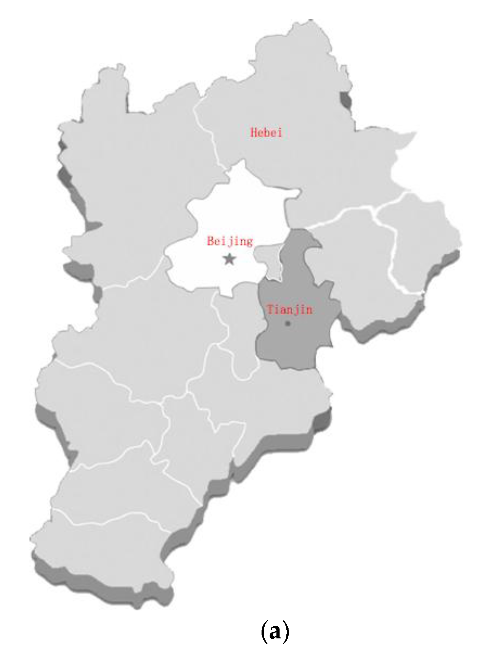
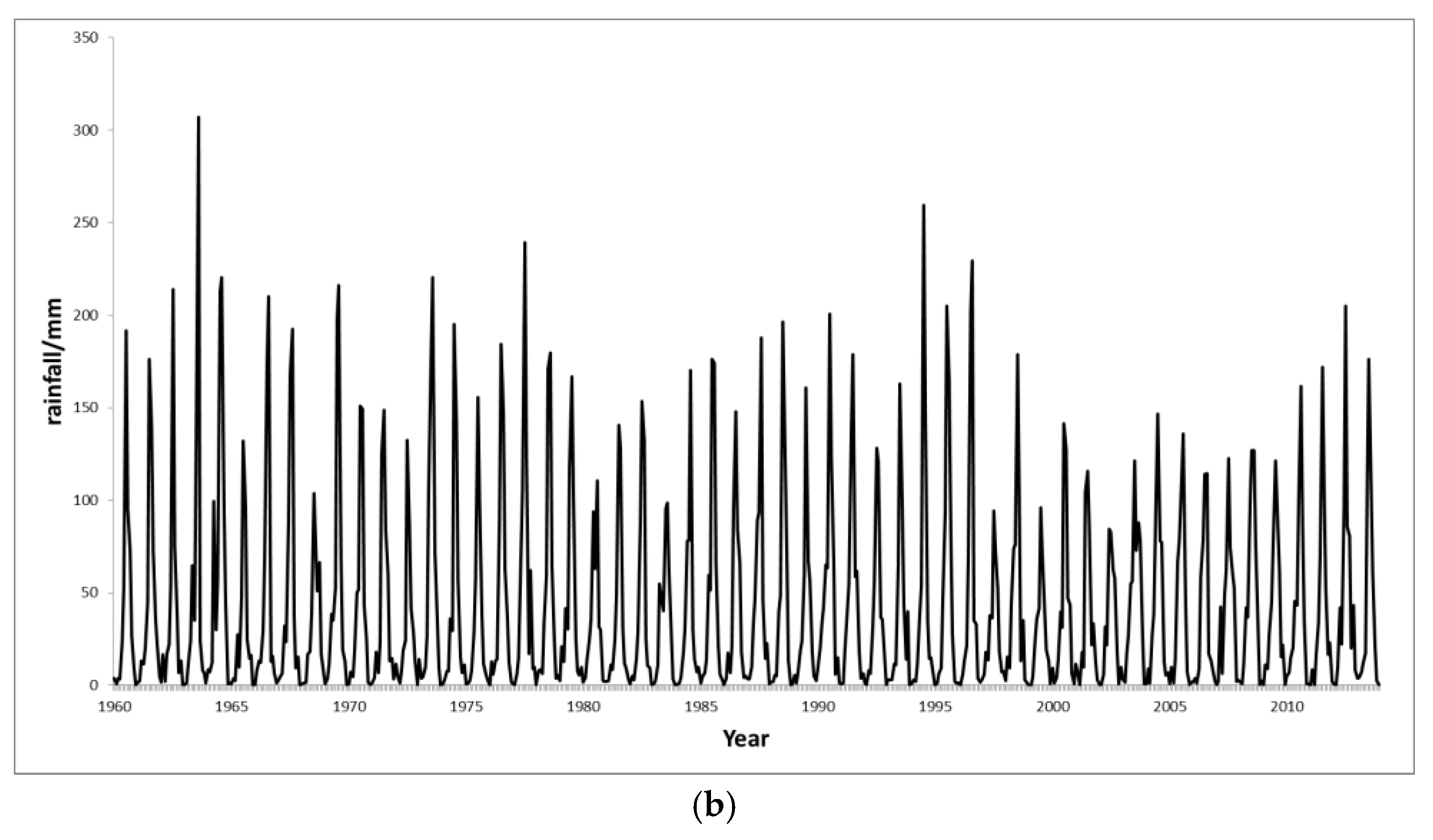
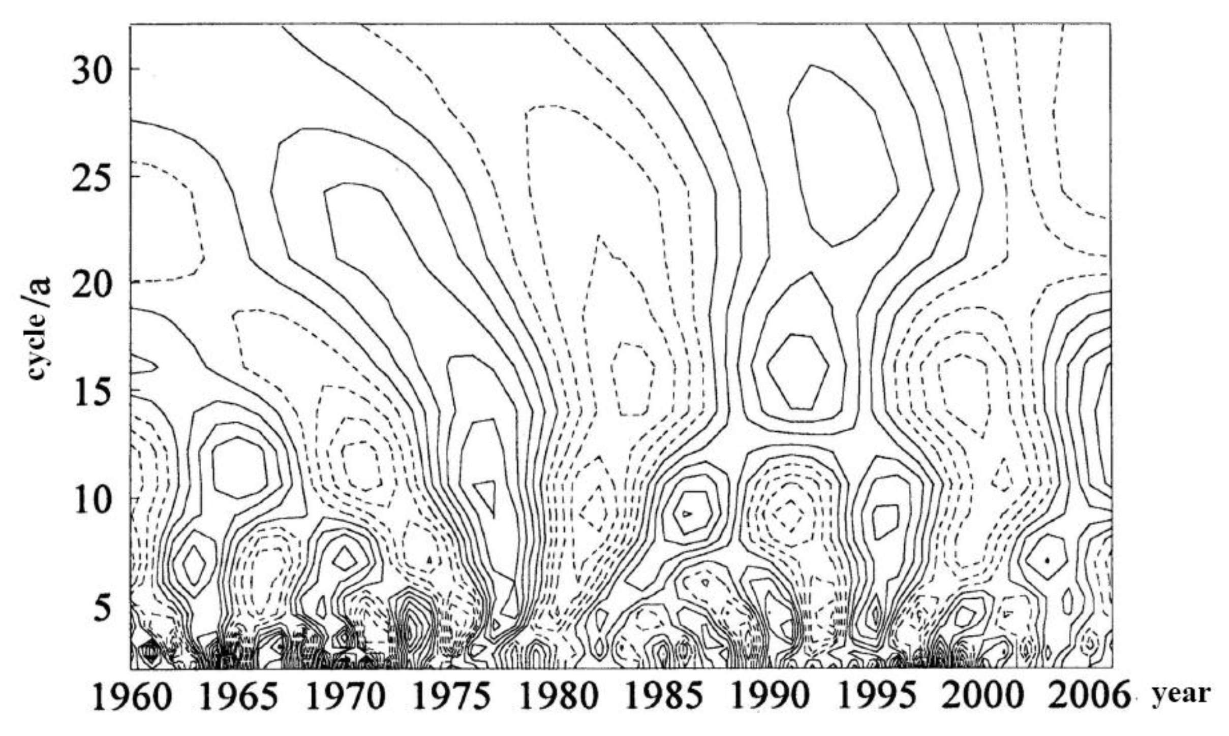
2.1. Research Data

The Beijing–Tianjin–Hebei region is located on the east coast of Eurasia, mid-latitude coastal and inland transfer zone. Influenced by a temperate climate with alternating moist and dry seasons, the annual rainfall in this area ranges from 400 to 800 mm. The study analyses the rainfall from 1969 to 2010 in the Thiessen rainfall station and the forecast is conducted based on the data of rainfall from the Taisen Station in the Beijing–Tianjin–Hebei region. Based on the Taisen Station rainfall data, the forecast is conducted. The results show that improved ant colony fuzzy clustering can effectively select historical data and improve the accuracy of prediction.
On the basis of the data of rainfall from 26 stations, the weight is determined by the Thiessen polygon method, and the weighted average rainfall data sequence is obtained. The Beijing–Tianjin–Hebei administrative divisions and the change of monthly rainfall from 1960 to 2013 in this area are shown in Figure 1.
Figure 2 gives the results of the wavelet analysis of the data from 1960–2006. Wavelet analysis is a localized analysis of the time (space) frequency. It multiplies the signal (function) step by step through the telescopic translation operation, finally reaches the time subdivision at high frequency, subdivides the frequency at low frequency, and can automatically adapt to the data analysis.
There are four obvious characteristic time scales, namely, 3a, 9a, 14a and 24a, respectively, where the characteristic time scale of 3a is always present from 1960–2006 and the period oscillation is stable. What is more, with 24a time scale cycle time oscillation throughout the study period, the performance is relatively stable. In the middle of the 1960s, Beijing–Tianjin–Hebei area had experienced four dry and wet alternations: from the mid-1960s to the late 1970s, the precipitation was abundant. In the 1980s, the precipitation was relatively low. In the 1990s, the precipitation again entered an abundant period. After the 21st century, the precipitation began to decrease. The characteristics of the two feature scales, 9a and 14a, are similar. Before the mid-1970s, the oscillation of the cycle time was more obvious, and after the rich period of 1970 to 1980, there was a slight increase in the feature scale, respectively, about 10a and about 15a.
The analysis reveals that the periodic variation of rainfall is obvious. Therefore, it is important to predict the future rainfall by grasping the key information of the rainfall in the historical year and using the data mining technology to classify the rainfall-related data reasonably.

2.2. An Introduction of Ant Colony Algorithm

We take the Travelling Salesman Problem (TSP) as an example to illustrate Ant Colony (AC) Algorithm. Suppose there are m cities, dij is the distance between city i and city j. τij(t) is the amount of information between city i and city j at time t. We use it to simulate the actual ant anterin, set a total of m ants, the term pij(t) represents the probably of the k-th ant being transferred between city i and city j at time t:
p i j ( t ) = τ i j a ( t ) η i j b ( i , k ) S , k U τ i k a ( t ) η i k b
where U is the part of the path that the ants have searched for, and S is the set of cities that the next step of the ant k allowed to pass, a indicates the amount of information on the path to the path chosen by the ants, ηij indicates the degree of transfer expectation between city i and j. When a = 0, the algorithm is the traditional greedy algorithm; and when b = 0, it becomes a pure positive feedback heuristic algorithm. After n moments, the ants can finish all the cities and complete a cycle. In this case, the amount of information on each path is updated according to the following formula:
τ i j n e w = ( 1 ρ ) τ i j o l d + Δ τ i j
where ρ ∈ (0, 1) represents the amount of information that fades with time. The information increment is expressed as:
Δ τ i j = k = 1 m Δ τ i j k
where Δ τ i j k is the amount of information left by ant k between city i and j. It can be expressed as:
Δ τ i j k = { Q / L k , i , j S 0 , otherwise
where Q is a constant and Lk is the length of the path traveled by the ant k in this cycle. After several cycles, the calculation can be terminated according to the appropriate stop condition.

2.3. Basic Principles of Fuzzy Clustering

Among the many fuzzy clustering algorithms, the most widely used and successful is Fuzzy C-means (FCM). The FCM algorithm divides n vectors xk (k = 1, 2, …, n) into m fuzzy clusters and obtains the clustering center of each cluster so that the objective function is minimized. The objective function is defined as:
J = k = 1 n i = 1 m ( μ i k ) h d ( x k , c i )
where μij is the membership function, ci is the i-th clustering center, h is the fuzzy weight index. μij ∈ (0, 1) and:
i = 1 m μ i k = 1
d ( x k , c i ) = | | x k c i | |
In order to minimize the objective function, the update of the cluster center and membership function is as follows:
c i = k = 1 n μ i k h x k k = 1 n μ i k h
μ i k = 1 j m ( d i k / d j k ) 1 / ( h 1 )
Since the solution of a multi-constrained optimization problem is complex, the commonly used method is to fix one of the parameters to optimize the other amounts, and the solution alternates until the difference between two consecutive functions is less than a very small value (the precision requirement).
The flaw of this algorithm is that it needs to be given multiple c values for repeated calculations, and the result is usually a local optimal solution, and the computation time is large because the time required for a matrix multiplication is O(n3), the time complexity of the first step of the algorithm is reached O(n4logn).

2.4. Improvement of Fuzzy Clustering by Ant Colony Algorithm

One of the keys to improve the speed of fuzzy clustering is to select the initial point of the membership function. If we can get the membership degree approximation result of each parameter point to each cluster, we will improve the speed of the fuzzy clustering algorithm and the ant colony algorithm can achieve this function.
The basic idea is to treat the data as an ant with different attributes. The clustering center is regarded as the “food source” that the ants are looking for, so the data clustering is seen as the process of the ant looking for food sources. The specific process can be described as follows: each ant travels from each cluster center, searches for the next sample point in the entire solution space, and then starts from the cluster center and searches for another sample point in the entire solution space. When the sample point reaches the total number of the original sample points of the cluster, the ant is considered to have completed a search for a path so that the ants do not repeat the same sample point in the search for the same path and set a taboo for each ant tabu(N). If tabu(N) = 1, then the node j can choose the search sample point, when the ants selected the node j, tabu(N) will be set 0, then the ants cannot choose the node.
Assume X = {Xi|Xj = (xi1, xi2, …, xim)}, i = 1, 2, …, n} is a collection of data to be clustered, τij(t) is amount of information between Xi and Xj at time t. When all the ants have completed a path search, it is said the algorithm carried out a search cycle. In the t search period, the path selection probability can be expressed as:
p i j ( t ) = { τ i j a ( t ) η i j b ( i , s ) S , k t a b u ( j ) τ i s a ( t ) η i s b , j = 1 , 2 , , m 0 , otherwise
where S = {Xs|dsjrj, s = 1, 2, …, N}, and the other parameters are consistent with the above.
When the i value is determined, make j from 1 to m, search the maximum pij(t), then Xi is merged into the Xj field. Make Cj = {Xi|dij < rj, i = 1, 2, …, k}, Cj represents all the data sets that are merged into Xj, and we find the cluster center:
c ¯ j = 1 k i = 1 k X i
When the ant colony completes a search period, the probability of each parameter point attributed to a cluster is obtained according to pij(t), and the general initial value of the fuzzy clustering membership matrix is obtained, and c ¯ j is used as the initial of fuzzy clustering center.
As the ant colony algorithm itself has a certain computational complexity, each fuzzy clustering cycle using multiple ant colony algorithm will produce over optimization phenomenon. We adopt the following strategy: in the first initial cycles, we use ant colony algorithm to determine the initial value pij(t) (in this paper we set 4 cycles) and c ¯ j , then iterate according to Equations (8) and (9). When the optimization process slows down, we use the ant colony algorithm once or twice to optimize until the accuracy requirements are reached.

2.5. Method Validation

In terms of monthly rainfall, the relevant factors include historical monthly mean temperature, mean air pressure, mean humidity, season etc. Because it is the region’s total rainfall forecast, we do not take into account the effects of terrain and ocean currents.
In this way, a five-dimensional vector is formed, namely monthly rainfall, monthly average temperature, monthly mean humidity, monthly mean pressure, seasonal type. Through the fuzzy clustering, the historical data will be grouped to form a database. In this way, when we predict future weather data more precisely, we can search from the historical database to find useful data for rainfall forecast. For seasonal data, we need to map the value, as shown in Table 1.
In order to test the performance of the algorithm, on a computer with the processor i7, memory 4g, the membership degree matrix is simulated. The first is to generate (0, 1) random number, the second is to use ant colony optimization (that is pij(t)). When calculating pij(t), set ρ = 0.7, a = 1, b = 1, η = 1, τij(0) = 0. The results are shown in Figure 3.
Figure 3a shows that the fuzzy clustering with the random number as the initial value of the membership matrix increases rapidly with the increase of the data volume, while the fuzzy clustering algorithm with pij(t) improves the number of samples with the increase of the number. Figure 3b shows that when the error rate is large, the random number and fuzzy clustering calculation using pij(t) are not very different, but when the error rate becomes smaller, the pij(t) fuzzy clustering is not changed, and the fuzzy clustering using random number calculation time is rising rapidly. Therefore, the clustering method adopted in this paper is more scientific and effective.

3. Rainfall Forecasting Model Based on CE

The historical data is huge and contains useful data. There are some abnormal data, so we have to choose specific methods according to actual situations in order to ensure the accuracy of the forecast. It is important to predict the future rainfall by grasping the key information of the rainfall in the historical year and using the data mining technology to classify the rainfall-related data reasonably; So Fuzzy Clustering by Ant Colony Algorithm is used for data clustering and the historical data are classified.

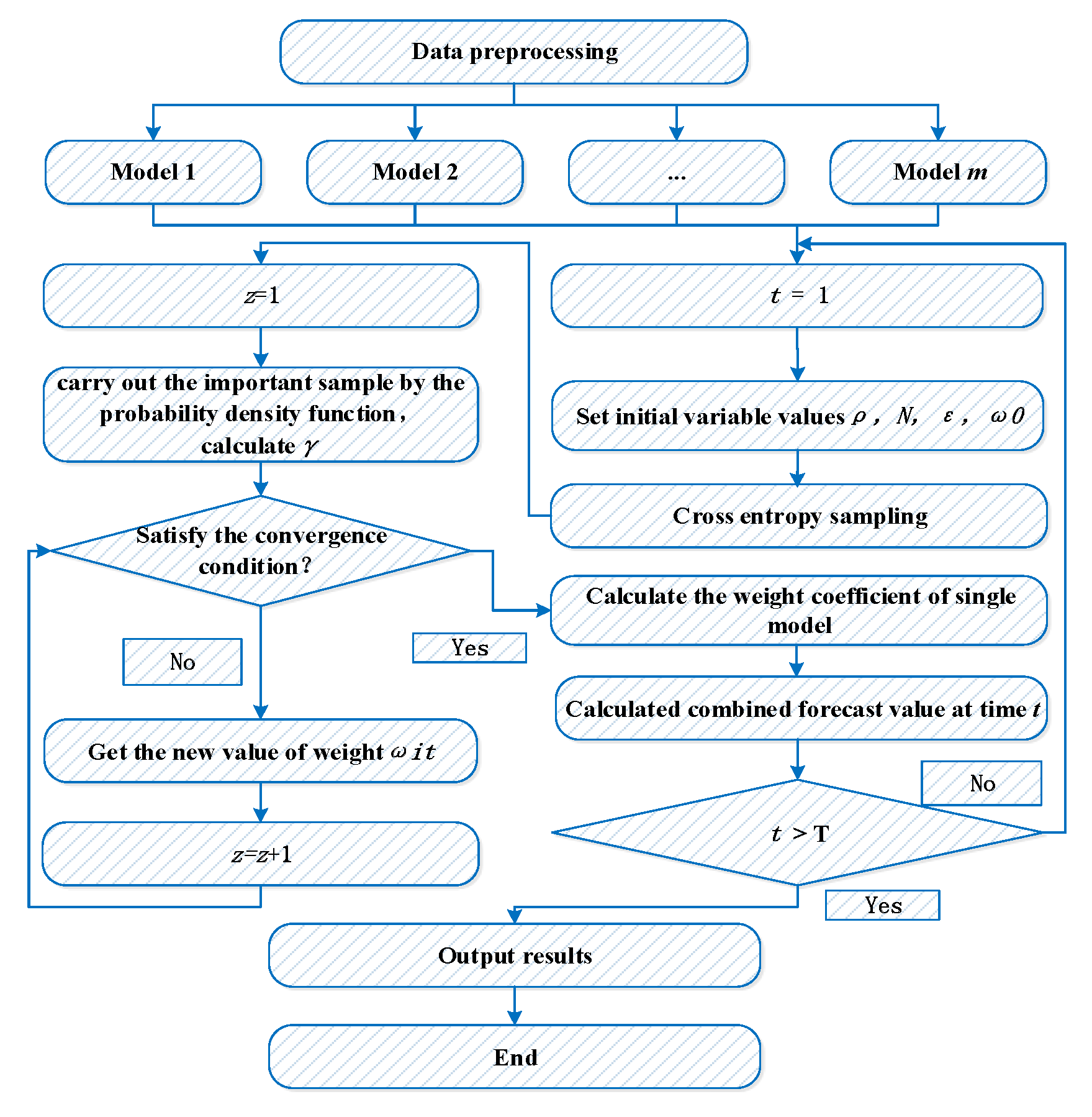
3.1. Combined Forecasting Model

The combined forecasting model comprises m single forecasting models and the relative effectiveness of a single forecasting model determined by the historical data. If the combined forecast value at time t is yt, ωij is the weight of the i-th model at time t, and y ^ i t is the predicted value of the i-th model at time t, then the problem of combined forecasting is described as follows:
y t = i = 1 m ω i t y ^ i t
Here two factors influence the final results of combined forecasting: a single model and the weight of a single forecasting model. In this study, we focus on the latter.
There are no uniform rules for selecting a single method, but instead we must consider the actual problem and the needs of the model. The factors considered in this study include: independence, diversity, and the accuracy of the algorithm. We use a single forecasting method to include the ARIMA time series model, GM, and the RBF.

3.2. The CE Model

According to the definition of entropy, a method for calculating the difference in information between two random vectors is defined as the CE. The CE model determines the extent of the mutual support degree by assessing the degree of intersection between different information sources. Moreover, the mutual support degree can be used to determine the weights of the information sources, where a greater weight represents higher mutual support. This is also called the Kullback-Leibler (K-L) distance. The CE of two probability distributions is expressed as D(f||g) [26,27].
For the discrete case:
D ( g | | f ) = 1 n g i ln g i f i
and for the continuous case:
D ( g | | f ) = g ( x ) ln g ( x ) f ( x ) d x = g ( x ) ln g ( x ) d x g ( x ) ln f ( x ) d x
where D ( g | | f ) represents the f to g distance, and f and g denote the probability vector in the discrete case and the probability density function in the continuous case, respectively.
The CE model quantifies the “distance” between the amounts of information. However, the K-L distance is not the real length distance, but instead it is the difference between two probability distributions. In this paper, g is the combined forecast function, f is the single method. CE value should be smallest when two pdf are identical. For the combined forecasting model based on CE, the CE model represents the support for combined forecasting. Therefore, the objective function is to assign weights between different single methods, so that there is the most similar case between the total predictive function and the true value.
To use the CE model, two major problems should be solved: establishing the probability density function and generating the CE objective function and solving the weight coefficient by iteration.
The rainfall is treated as a sequence of discrete random variables in the forecast period. For a certain point in the sequence, the value of the rainfall at a certain prediction time is continuous, so it can be regarded as a continuous random variable. Therefore, rainfall prediction can be treated as a sequence of discrete times but continuous values.
The probability density function for predicting rainfall f(x) can be regarded as the probability density function fi(x) of the single forecasting method multiplied by the corresponding weight. According to the central limit theorem, if a variable is the sum of many independent random factors, we can treat the variable as following a normal distribution, and thus the rainfall value at a certain time can be considered as satisfying a normal distribution. The minimum CE is used to determine the probability distribution of the different forecasting methods, so the combined probability distribution of the rainfall is obtained.
The probability density function for method i is (i = 1, 2, …, m):
f i ( x ) = 1 2 π σ i e ( x μ i ) 2 / ( 2 σ i 2 )
where μi is the mean value and σi is the variance.
Thus, the combined probability density function of the predicted rainfall can be obtained based on the probability density function of the single prediction method:
f ( x ) = i = 1 m ω i t f i ( x )
where ωij is the weight of the i-th single method.
Therefore:
f ( x ) ~ N ( i m ω i t μ i t , i m ( ω i t σ i t ) 2 )
From (17), the objective function of the minimum CE optimization problem is set as:
min F = min D ( f i ( x ) | | f ( x ) )
s.t.
{ 0 ω i t 1 i = 1 m ω i t = 1
Selecting the appropriate weight vector to obtain the minimum F involves determining the support for different algorithms.
The weight coefficient is derived based on the Lagrange function method. The K-L distance can be transformed into a sampling function g*(x) and f(x;ωij) to ensure that g ( x ) ln f ( x ; ω i t ) d x reaches the minimum value, which is equivalent to the maximum value problem:
max g ( x ) ln f ( x ; ω i t ) d x
where:
g ( x ) = I { S ( x ) > γ } f ( x , ω 0 ) l
and I{S(x)>γ} is called the indicator function:
I { S ( x ) > γ } = { 1 ,  S ( x ) > γ 0 ,  S ( x ) γ
where S(x) is also f(x;ωij), ω0 is the initial weight, γ is the target estimation parameter, and L represents the estimated target value of a low probability event.
Based on the idea of CE, a low probability sampling method is used to convert the optimization problem into the following CE problem:
max D ¯ ( ω i t ) = max 1 N k = 1 N I { S ( x ) > γ } ln f ( x k ; ω i t )
where N is a random number of samples.
Note that i = 1 m ω i t = 1 , and thus we can construct a Lagrange function:
H ( x ) = 1 N k = 1 N I { S ( x ) > γ } ln f ( x k ; ω i t ) + λ ( i = 1 m ω i t 1 )
where λ is the Lagrange multiplier.
Note that:
ln f ( x k ; ω i t ) = i = 1 m ( x k μ i t ) 2 2 σ i t 2 ln ω i t 2 π σ i t
By taking the partial derivative to ωij and λ to zero, we can obtain:
ω i t = π 2 k = 1 N I { S ( x ) > γ } ( x k μ i t ) 2 N σ i t λ
By substituting this into i = 1 m ω i t = 1 , we can obtain:
λ = 1 N π 2 i = 1 m k = 1 N I { S ( x ) > γ } ( x k μ i t ) 2 N σ i t
The expression for the weight coefficient is obtained as follows:
ω i t = k = 1 N I { S ( x ) > γ } ( x k μ i t ) 2 σ i t i = 1 m k = 1 N I { S ( x ) > γ } ( x k μ i t ) 2 σ i t
Iterative process:
A. Set t = 1;
B. Set wit = w0, set iteration number z = 1;
C. Generate sample sequence X = { X 1 , X 2 , , X N } by f ( x ; ω i t ) , and sort it from small to large, calculate S ( x k ) = f ( X k , ω i t ) , and thus the estimated value γ is:
γ ( z ) = f ( X 1 ρ ; ω i t )
D. Calculate (27) and obtain the z-th iteration result ω i t ( z ) . Set z = z + 1;
E. Return to Step B to obtain γ ( z ) , and calculate | γ ( z ) γ ( z 1 ) | . If the results is less than a certain error ε , return to F; otherwise, return to C;
F. Stop the iterations, where ω i t ( z ) is the optimal weight and the rainfall prediction value is
f t = i = 1 m ω i t ( z ) f i t
G. Set t = t + 1. Assess whether t is less than or equal to T. If yes, return to step 2 to calculate some combined forecast values at other times; if not, finish the computation.
The overall forecasting process is shown in Figure 4.

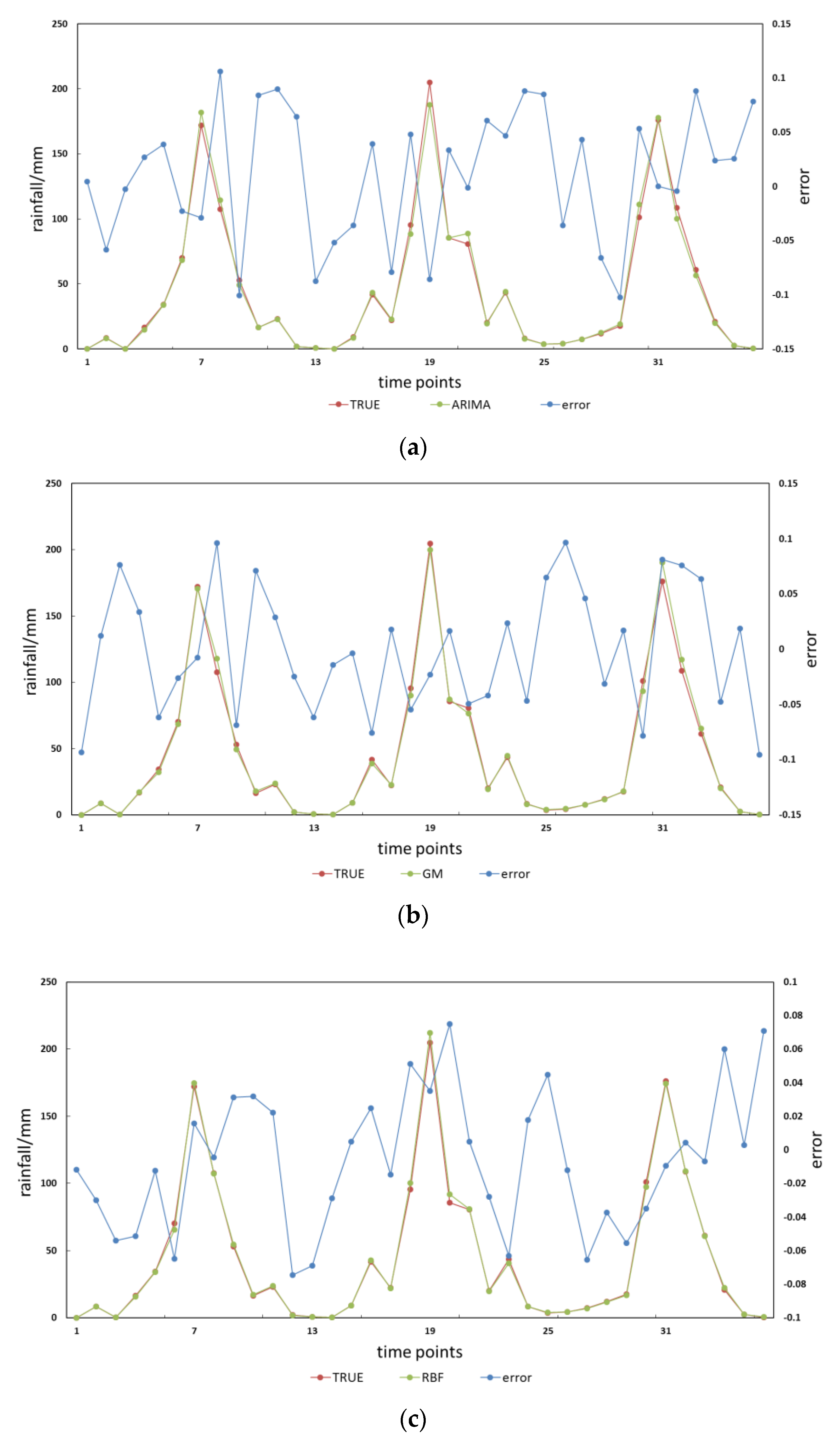
4. Results and Analysis

This study selects the monthly and annual rainfall data from 1960–2010 as training samples and chooses the rainfall data from 2011–2013 as test samples. Then a monthly rainfall forecast is carried on. The selected single models include ARIMA, GM, RBF, CE. The performance of the single forecasting model and combined forecasting model is characterized by Root mean squared error (RMSE) and Maximum relative percentage error (MRPE).

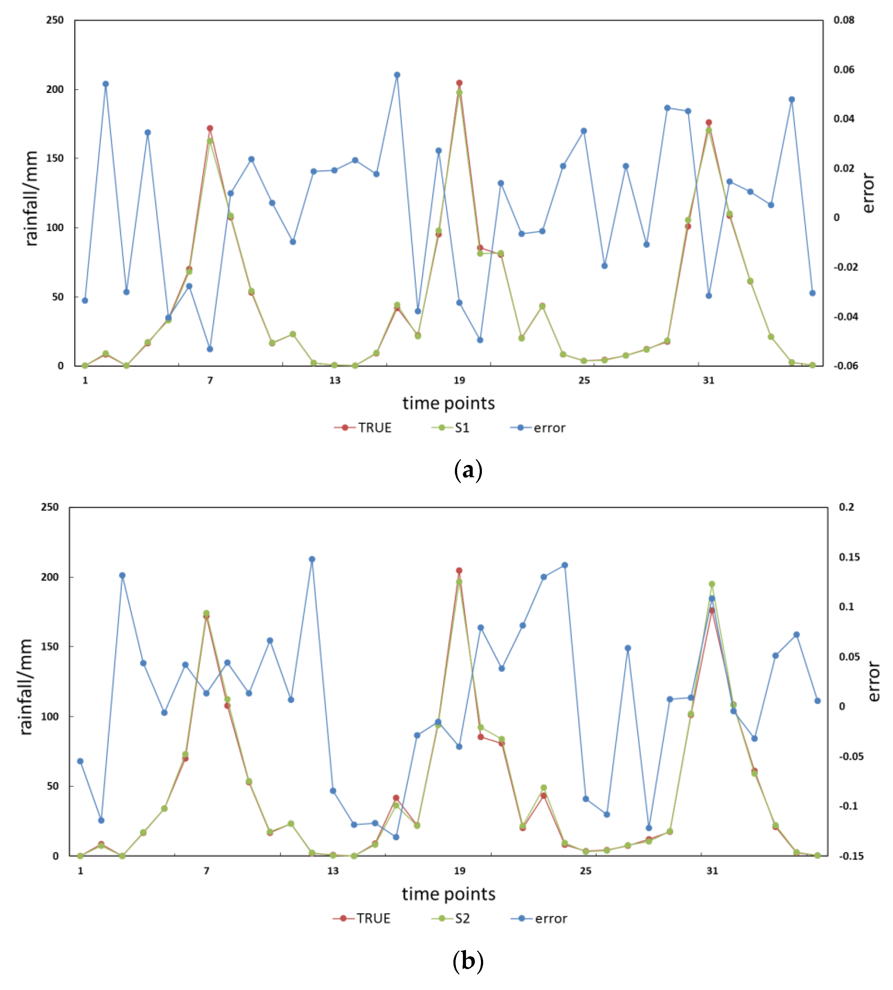
4.1. Predictive Stability Comparison Results

After the single algorithm is determined, the rainfall from 2011 to 2013 is predicted and the absolute error is calculated. To compare the stability of various algorithms, true value, predictive value and the absolute error trend curve (a total of 36 prediction points) are shown as follows:
From Figure 5, it is clear that in a single algorithm, the absolute error of prediction is large or small, and stable results cannot be maintained over a long time scale. As a result, the reliability is not high; in combined prediction, the absolute error is relatively flat, which greatly improves the stability of prediction. The prediction results are more authentic. The error analysis of the results of the 2011–2013 is shown in Table 2.
From Table 2 and Figure 5 it can be seen that: (1) compared to a single method of RMSE, the combination of forecasting methods in a certain prediction point may not be optimal, but the overall error is small compared with GM, ARIMA, RBF of RMSE, and the error reduces. The combined forecasting method has a higher accuracy: in the average MRPE index, compared to ARIMA, GM, RBF, CE reduces error of 2.11%, 1.73%, 0.1%; in the average RMSE index, compared to ARIMA, GM, RBF, CE were reduced by 1.74%, 1.08%, 0.43%; (2) the MRPE index in a single method can be very high (MRPE of GM in 2012), and there is a risk of failure of the model. The combined forecasting method greatly reduces the maximum error, and has better prediction stability (MRPE of CE in 2012); (3) in a single method, the prediction error sometimes is large, the error of the combined forecast will be also relatively large (for example in 2012), and the accuracy of the single forecasting model has a certain effect on the accuracy of the combined model.

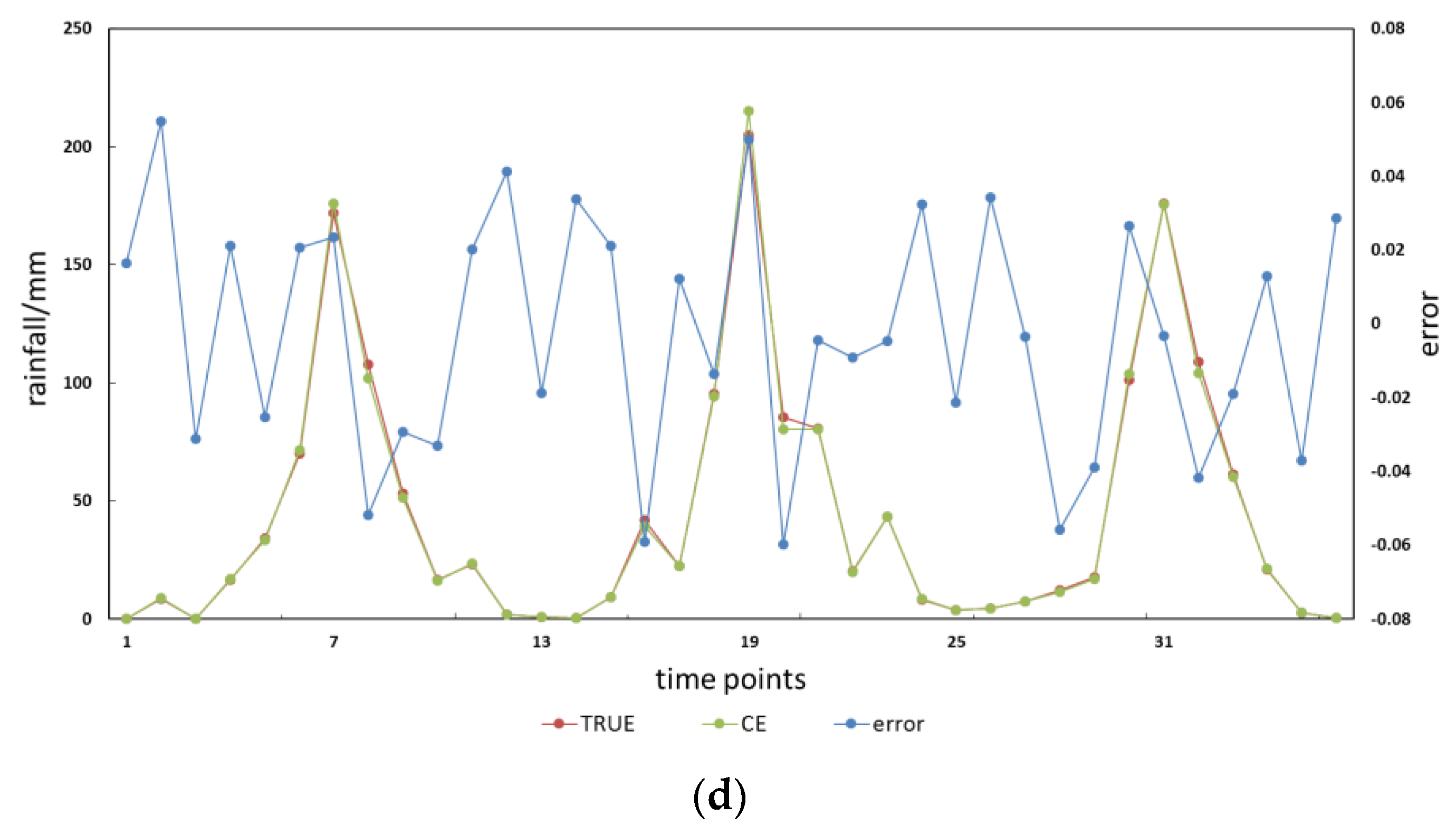
4.2. The Influence of Clustering Method on Prediction Results

To illustrate the effect of clustering on the accuracy of prediction, two scenarios are created:
  • Scenario 1: Traditional c-means clustering method
  • Scenario 2: We do not cluster historical data.
The error results are shown in Table 3 and Figure 6.
From the comparison between Table 2 and Table 3, it is easy to know that the clustering method used in this paper is consistent with the accuracy of traditional clustering method to meet the forecasting requirements. In the average MRPE index, compared to S1, S2, the clustering method used in this paper reduces the error by 0.01%, 3%; in the average RMSE index, compared to ARIMA, GM and RBF, CE were reduced by 0.05%, 1.08%, 3.52%. However, from Figure 3, the method has great advantages in calculating the speed when the data volume is large. In addition, comparing with the case of S2, we can see that there is a large deviation in the result of prediction in the case of no clustering, which indicates that the selection of historical data has important influence on the precision of prediction and it is necessary to fully excavate and classify the historical information to reach reasonable effect.

5. Conclusions

Because the meteorological conditions are stochastic, the rainfall variation is a non-stationary time series, and the accuracy of prediction and reliability of traditional single forecasting methods cannot be ensured. The combined forecasting model based on CE is proposed to solve these problems. Besides, the forecasting results of several single methods are used as the input variables for training, and the output weights are predicted by analyzing the total rainfall. The simulation results show that the combined forecasting model enhances the accuracy and reliability of the rainfall forecasting model. Additionally, clustering method is modeled and analyzed so as to improve the accuracy of prediction. The results demonstrate that the accuracy of combined forecasting can be improved by using the fuzzy clustering. The chosen method characterizes the change laws of the rainfall well and to improve the stability of the prediction. The prediction results can help agriculture, water conservancy departments to improve the ability of drought and flood disaster prevention and control. In the future, more steps can be taken for improvement: (1) the single forecasting method with higher accuracy and more suitable single forecasting method should be chosen and the accuracy of combined model prediction should be further improved to explore the rule of selecting different single methods in combined forecasting method; (2) the data in similar year should be collected to predict and historical data should be utilized more effectively so that the result is more scientific and convincing.

Acknowledgments

This work was supported by the National Key R&D Program of China (Grant No. 2016YFC0401406), and the Famous Teachers Cultivation planning for Teaching of North China Electric Power University (the Fourth Period), the 2014 Education Reform Project of North China Electric Power University (Beijing Department) (Grant No. 2014JG57).

Author Contributions

The combined forecasting method based on SVM was developed to forecast the rainfall. The results demonstrate that this model can improve the accuracy of daily rainfall forecasting and it can be applied in practice. Baohui Men designed the study, Rishang Long and Yangsong Li performed the experiments and wrote the paper, Baohui Men reviewed and edited the manuscript. All authors read and approved the manuscript.

Conflicts of Interest

The authors declare no conflict of interest.

References

  1. Serreze, M.C.; Etringer, A.J. Precipitation characteristics of the Eurasian Arctic drainage system. Int. J. Climatol. 2003, 23, 1267–1291. [Google Scholar] [CrossRef]
  2. Bustamante, J. Evaluation of April 1999 Rainfall Fore-casts Over South American using the Eta Model Climanalise, Divulgacao Científica. Cachoeira Paulista 1999, 6, 3563–3569. [Google Scholar]
  3. Black, T. The New NMC Mesoscale ETA Model: Descriptionand Forecast Examples. Whether Forecast. 1994, 9, 265–278. [Google Scholar] [CrossRef]
  4. Mossad, A.; Alazba, A.A. Drought Forecasting Using Stochastic Models in a Hyper-Arid Climate. Atmosphere 2015, 6, 410–430. [Google Scholar] [CrossRef]
  5. Bian, H.J.; Lei, H.J.; Wang, Y. Application of Grey Theory to Regional Rainfall Rorecast. Anhui Agri. Sci. 2009, 37, 6059–6060. [Google Scholar]
  6. Yang, J.L.; Wu, Y.N.; Xie, M.; Li, H.Y. Application of Monte Carlo Method in Rainfall Forecast of Flood Season in Nenjiang Basin. S. N. Water Transf. Water Sci. Technol. 2011, 9, 28–32. [Google Scholar]
  7. Ramirez, M.C.V.; de Campos Velho, H.F.; Ferreira, N.J. Artificial Neural Network Technique for Rainfall Forecasting Applied to the Sao Paulo Region. J. Hydrol. 2005, 301, 146–162. [Google Scholar] [CrossRef]
  8. Manzato, A. Sounding-derived indices for neural network based short-term thunderstorm and rainfall forecasts. Atmos. Res. 2007, 83, 349–365. [Google Scholar] [CrossRef]
  9. Yang, S.; Rui, J.; Feng, H. Application of Support Vector Machine (SVM) Method in Precipitation Classification Forecast. J. Southwest. Agric. Univ. 2006, 28, 252–257. [Google Scholar]
  10. Cui, L.; Chi, D.; Qu, X. Based on Wavelet De-noising of Stationary Time Series Analysis Method in Rainfall Forecasting. China Rural Water Hydropower 2010, 9, 31–35. [Google Scholar]
  11. Merlinde, K. The Application of TAPM for Site Specific Wind Energy Forecasting. Atmosphere 2016, 7, 23. [Google Scholar] [CrossRef]
  12. Lauret, P.; Lorenz, E.; David, M. Solar Forecasting in a Challenging Insular Context. Atmosphere 2016, 7, 18. [Google Scholar] [CrossRef]
  13. Men, B.; Liu, C.; Xia, J.; Liu, S.; Lin, Z. Application of R/S Analysis Method of Water Runoff Trend in West Route of South-to-North Water Transfer Project. J. Glaciol. Geocryol. 2005, 27, 568–573. [Google Scholar]
  14. Soro, G.E.; Noufé, D.; Goula Bi, T.A.; Shorohou, B. Trend Analysis for Extreme Rainfall at Sub-Daily and Daily Timescales in Côte d’Ivoire. Climate 2016, 4, 37. [Google Scholar] [CrossRef]
  15. Chen, C.-S.; Duan, S.; Cai, T. Short-term photovoltaic generation forecasting system based on fuzzy recognition. Trans. China Electrotech. Soc. 2011, 26, 83–88. [Google Scholar]
  16. Liu, Y.; Fu, X.; Zhang, W. Short-term load forecasting method based on fuzzy pattern recognition and fuzzy cluster theory. Trans. China Electrotech. Soc. 2002, 17, 83–86. [Google Scholar]
  17. Kolentini, E.; Sideratos, G.; Rikos, V. Developing a Matlab tool while exploiting neural networks for combined prediction of hour’s ahead system load along with irradiation, to estimate the system loadcovered by PV integrated systems. In Proceedings of the IEEE Conferences on Clean Electrical Power, Capri, Italy, 9–11 June 2009; pp. 182–186. [Google Scholar]
  18. Bates, J.; Granger, C. The combination of forecast. Oper. Res. Q. 1969, 20, 451–468. [Google Scholar] [CrossRef]
  19. Wu, Q.; Peng, C. Wind Power Generation Forecasting Using Least Squares Support Vector Machine Combined with Ensemble Empirical Mode Decomposition, Principal Component Analysis and a Bat Algorithm. Energies 2016, 9, 261. [Google Scholar] [CrossRef]
  20. Pedersen, J.W.; Lund, N.S.V.; Borup, M.; Löwe, R.; Poulsen, T.S.; Mikkelsen, P.S.; Grum, M. Evaluation of Maximum a Posteriori Estimation as Data Assimilation Method for Forecasting Infiltration-Inflow Affected Urban Runoff with Radar Rainfall Input. Water 2016, 8, 381. [Google Scholar] [CrossRef]
  21. Box, G.E.P.; Jenkins, G.M. Time Series Analysis, Forecasting and Control; Holden-Day: San Francisco, CA, USA, 1976. [Google Scholar]
  22. Men, B.; Long, R.; Zhang, J. Combined Forecasting of Stream flow Based on Cross Entropy. Entropy 2016, 18, 336. [Google Scholar] [CrossRef]
  23. Cui, D. Application of Combined Model in Rainfall Forecast. Comput. Simul. 2012, 29, 163–166. [Google Scholar]
  24. Xiong, L.; O’Connor, K.M.; Kieran, M. Comparison of four updating models for real-time river flow forecasting. Hydrol. Sci. J. 2002, 47, 621–640. [Google Scholar] [CrossRef]
  25. Lu, C.; Zhang, Y.; Zhou, J.; Vijay, P.; Guo, S.; Zhang, J. Real-time error correction method combined with combination flood forecasting technique for improving the accuracy of flood forecasting. J. Hydrol. 2015, 521, 157–169. [Google Scholar]
  26. Singh, V.P. Entropy Based Parameter Estimation in Hydrology; Kluwer Academic Publishers: Dordrecht, The Netherlands, 1998. [Google Scholar]
  27. Cui, H.; Singh, V.P. Entropy spectral analyses for groundwater forecasting. J. Hydrol. Eng. 2017, 22, 06017002. [Google Scholar] [CrossRef]
  28. Chen, L.; Singh, V.P.; Xiong, F. An Entropy-Based Generalized Gamma Distribution for Flood Frequency Analysis. Entropy 2017, 19, 239. [Google Scholar] [CrossRef]
  29. Chen, L.; Singh, V.P. Generalized Beta Distribution of the Second Kind for Flood Frequency Analysis. Entropy 2017, 19, 254. [Google Scholar] [CrossRef]
  30. Chen, L.; Singh, V.P.; Guo, S.L.; Zhou, J.; Ye, L. Copula entropy coupled with artificial neural network for rainfall-runoff simulation. Stoch. Environ. Res. Risk Assess. 2014, 28, 1755–1767. [Google Scholar] [CrossRef]
  31. Li, R.; Liu, H.L.; Lu, Y.; Han, B. A combination method for distribution transformer life prediction based on cross entropy theory. Power Syst. Prot. Control 2014, 42, 97–101. [Google Scholar]
  32. Chen, N.; Sha, Q.; Tang, Y.; Zhu, L. A Combination Method for Wind Power Predication Based on Cross Entropy Theory. Proc. CSEE 2012, 32, 29–34. [Google Scholar]
  33. Mehdi, N.; Hossein, N. Image denoising in the wavelet domain using a new adaptive thresholding function. Neurocomputing 2009, 72, 1012–1025. [Google Scholar]
  34. Asgari, M.S.; Abbasi, A. Comparison of ANFIS and FAHP-FGP methods for supplier selection. Kybernetes 2016, 45, 474–489. [Google Scholar] [CrossRef]
Figure 1. The Beijing–Tianjin–Hebei administrative divisions and change of monthly rainfall from 1960 to 2013. (a) Beijing–Tianjin–Hebei administrative divisions; (b) monthly rainfall from 1960 to 2013.
Entropy 19 00694 g001aEntropy 19 00694 g001b
Figure 2. Wavelet analysis of the rainfall data from 1960–2006.
Entropy 19 00694 g002
Figure 3. Clustering calculation time. (a) calculation time when error rate is constant; (b) calculation time when data amount is constant.
Entropy 19 00694 g003
Figure 4. Flowchart illustrating the algorithm.
Entropy 19 00694 g004
Figure 5. Prediction curve. (a) ARIMA; (b) GM; (c) RBF; (d) CE.
Entropy 19 00694 g005aEntropy 19 00694 g005b
Figure 6. Prediction curve. (a) S1; (b) S2.
Entropy 19 00694 g006
Table 1. Seasonal mapping values.
Month12, 1, 23, 4, 56, 7, 89, 10, 11
value0.10.30.50.7
Table 2. Error analysis of the results.
ARIMAGMRBFCE
MRPERMSEMRPERMSEMRPERMSEMRPERMSE
201112.13%5.53%11.15%4.49%10.99%4.21%10.02%3.93%
20129.44%4.99%13.15%4.97%8.65%5.01%9.45%4.32%
201311.10%7.12%7.22%6.19%7.01%4.49%6.88%4.17%
Average10.89%5.88%10.51%5.22%8.88%4.57%8.78%4.14%
Table 3. Influence of clustering method on prediction results.
S1S2
MRPERMSEMRPERMSE
201110.04%3.89%13.01%7.12%
20129.41%4.34%12.04%8.14%
20136.92%4.17%10.29%7.71%
Average8.79%4.19%11.78%7.66%

