Abstract
In the Bayesian framework, the usual choice of prior in the prediction of homogeneous Poisson processes with random effects is the gamma one. Here, we propose the use of higher order maximum entropy priors. Their advantage is illustrated in a simulation study and the choice of the best order is established by two goodness-of-fit criteria: Kullback–Leibler divergence and a discrepancy measure. This procedure is illustrated on a warranty data set from the automobile industry.
1. Introduction
In the study of the prediction problem for homogeneous Poisson processes (HPP), used in various fields including biomedicine [1], marketing [2] and reliability [3], the recurrent events often display extra-Poisson variation. In this problem, the variation is usually handled in an empirical Bayesian fashion and the gamma prior is the most common choice. In [4], we compared the performance of the 2-moment maximum entropy prior to other commonly used ones, estimating the parameters by matching moments (MM) [4,5,6,7,8,9,10] as well as maximum likelihood (ML) [6].
ML did as well as MM and often outperformed it. Unfortunately, the [8] result implies that only cases where the coefficient of variation is less than one can be considered with this 2-moment maximum entropy prior. Here, we use higher moment maximum entropy priors to overcome this restriction and, to the best of our knowledge, such priors have not been used for this problem. These priors are also quite versatile, including bimodality [11,12]. It should be noted that we always assume that each of the k-moments is finite.
Given the excellent performance of the maximum likelihood estimation method (MLE) for the 2-moment problem and its ease of computation compared to matching moments, especially when the number of moments is greater than 2, we choose to use MLE here and call it the MLE–MaxEnt method. The k-moment maximum entropy prior for the homogeneous Poisson process with random effects (HPPr) obviously outperforms the 2-moment maximum entropy prior, but we also compare it with other priors such as the gamma, which is popular among the conjugate priors and results in the negative binomial (NB) posterior distribution. It should be noted that the gamma distribution can also be considered as a maximum entropy distribution under different constraints [7].
The performance of the k-moment maximum entropy priors is evaluated using the Kullback–Leibler criterion [13] and a discrepancy measure equal to the root mean square prediction error between the predicted value obtained using a specific prediction model and the estimator obtained here using our methods [14].
The method using HPPr is also illustrated on a real example, a warranty data set from the automobile industry. Here, we use several different prediction models with k-moment entropy priors for different values of k. We study their performance using the absolute error discrepancy equal to the absolute difference between point predictors. We also use the likelihood ratio test as a stopping rule to determine an adequate value for k for the k-moment maximum entropy priors applied in the case of this example. A general discussion with concluding remarks is presented in Section 5.
The remainder of this paper is organized as follows. In Section 2, we describe the maximum entropy principle, recall the definition of a homogeneous Poisson process with random effects (HPPr) and introduce the general Poisson–MaxEnt model. In Section 3, the maximum likelihood approach to estimate the vector of parameters of this general Poisson–MaxEnt model is discussed. In Section 4, the performance of the k-moment maximum entropy priors for different values of k proposed here and their comparison with the use of the gamma conjugate prior are studied through Monte Carlo simulations. In order to test our methods, we used many different priors to generate the original random effects including the k-moment maximum entropy priors: the gamma, the generalized gamma, the Weibull, the lognormal, the uniform and the inverse gaussian.
2. The Homogeneous Poisson Process with Random Effects and the Maximum Entropy Principle
Here, we describe the maximum entropy principle, introduce the homogeneous Poisson process with random effects (HPPr) and define our general Poisson–MaxEnt model.
2.1. The Maximum Entropy Principle
As noted in our study [4], the entropy of a probability density is a measure of the amount of information contained in the density and was first defined by [15] as
The goal is to maximize H subject to certain conditions. The usual choice to determine is to use a finite set of expectations of known functions and to match these empirical moments. This is called the matching moment (MM) estimation method. These known functions are often the non-central moments of the form . In simple cases, using these non-central moments, maximizing the likelihood yields the same estimates as the matching moment method [6].
To find the function that maximizes the entropy of this nonlinear problem using matching moments, we form the Lagrangian, which we have assumed is finite:
where are the k non-central moments and is a vector of Lagrange multipliers.
Applying the Lagrange multiplication method [16], the following k-moment maximum entropy prior distribution is defined by:
where A is a normalization constant defined as follows:
2.2. Homogeneous Poisson Processes with Random Effects
We let represent the number of events occurring for a subject in the time interval with representing . To model such recurrent events, many different types of processes are discussed in the literature [17] where the Poisson process (PP) is one of the most popular ones. We will consider here only continuous time processes where two events cannot occur simultaneously. The number of events can be defined through the intensity function:
where denotes the history of the process up to time t.
The intensity function used to model these events corresponds to a homogeneous Poisson process with random effects (HPPr) where the rates are the unknown parameters. Suppose that we have n subjects and that denotes the number of events occurring for a subject i up to time t. When these processes are not time-homogeneous and there is more variation between the individual subjects in the recurrent events , then the are considered unobservable i.i.d. random effects and the random model is defined by:
where the processes are independent, , an unknown prior distribution for and each process is observed up to a fixed time . We want to estimate a point predictor for each . Throughout this article, , and will be denoted by , and respectively.
The choice of an appropriate prior distribution for is always a very delicate procedure in Bayesian analysis. It is not clear how to translate our beliefs about into a distribution . Although Bayesian analysis is often based on “non-informative priors” [18,19], there are convincing arguments against the existence of such priors. We prefer using the maximum entropy approach which makes use of prior information often given in the form of the expectations of some known functions to generate a maximum entropy prior. Such functions are often the non-central moments. The objective of this approach is to choose a prior probability distribution function for the which best represents this data. The Maximum Entropy Principle states that, given some constraints on the prior, the prior should be chosen to be the distribution with the largest entropy that follows these constraints.
For the prediction problem for HPPr, numerous researchers used the gamma distribution for the prior distribution [20]. The choice of the gamma distribution was motivated by mathematical convenience only since it is the conjugate prior of the Poisson distribution and results in the negative binomial (NB) posterior distribution. Moreover, in [4], we concluded that the 2-moment maximum entropy prior compared very favorably to the gamma prior in the prediction for HPPr. Here, we improve on these results by the use of the k-moment maximum entropy priors (). This is called the general Poisson–MaxEnt model.
2.3. Model Specification of the General Poisson–MaxEnt Model
The general Poisson–MaxEnt model with k-moments that we develop is then given by:
where is a normalization constant and is a vector of parameters. Clearly, must be positive.
For the Poisson–MaxEnt model (3), the joint posterior distribution of all the unknown parameters is given by
Hence, using this conditional density, the density function for is then given by
We note that the posterior distribution (4) will not have a known closed form, but includes rather complicated high dimensional densities, thus rendering direct inference almost impossible because of the high dimensional integration, necessary to obtain the normalizing constant, which is not mathematically tractable. For this reason, we generate from this posterior distribution a large number of samples using Markov chain Monte Carlo (MCMC) implemented in WinBUGS [21], and, from these samples, we can obtain appropriate parameter estimates such as the posterior mean of , where is estimated by the methods described in the next section.
3. Estimating Unknown Poisson–Maximum Entropy Parameters
The object of both estimation approaches, MM and MLE, in the general Poisson–Maximum Entropy model is to choose the probability distribution for the unknown vector of parameters that best represents the observed data .
Here, we favour the maximum likelihood method (the MLE–MaxEnt method) because it is computationally less complex than the MM method when . For completeness, the MM method for the MaxEnt–Poisson model will be described in Appendix A.
The MLE–Maximum Entropy Method for the Poisson–MaxEnt Model
Here, we introduce the MLE–Maximum entropy (MLE–MaxEnt) method using MLE for estimating the parameters of the empirical Bayes MaxEnt model (3). To obtain them, we construct the marginal likelihood L of the empirical Bayes general Poisson–Maximum Entropy model (3)
with
and is a normalization constant.
Ignoring the terms that do not depend on , the log-likelihood is given by
One method to find the maximum of (7) is to take the partial derivatives and set them equal to 0 [10]. The necessary and sufficient conditions to interchange the order of differentiation and integration of Lebesgue’s Dominated Convergence Theorem [22] are verified here for both (6) and the normalization constant . Interchanging differentiation and integration, the first derivatives of (7) with respect to are given by the following equations:
The analytic solutions to the equations in (8) are difficult to obtain; thus it is natural to use a numerical method to estimate directly the vector of parameters that maximize the log-likelihood (7).
We have chosen MATLAB (version 9.1 (R2016b), MathWorks, Natick, MA, USA) “fminsearchbnd”, a nonlinear optimization method which is derivative-free and allows bounds on the variables for this MLE problem. Under our model (3) for HPPr, matching moments and the MLE–Maximum entropy methods for Poisson–MaxEnt model will not yield the same estimates. This differs from the simple case without Poisson processes considered by Mohammad-Djafari [6].
4. Simulation Studies and Data Applications
4.1. Simulation Studies
Through extensive simulation studies presented in this section, we will study and compare the performance of our general Poisson–MaxEnt model with this k-moment prior () to the models using the 2-moment maximum entropy prior or the gamma prior where the parameters were estimated using the MLE method. For comparison, we use the following goodness-of-fit criteria: Kullback–Leibler distance and a discrepancy measure for point predictions equal to the root mean square prediction error.
Throughout this study, we know that one advantage of using the general Poisson–MaxEnt model with this k-moment prior () for prediction in HPPr is that it can be used regardless of the values of the coefficient of variation. It also allows us to reflect different orders of heterogeneity in the data. Among all results obtained with different values of the coefficient of variation, we only present here the results for two of them in order to be concise. The first one represents a case where the value of the coefficient of variation is less than 1 and the second where it is greater than 1. The latter case is used in order to show the benefit of using the general Poisson–MaxEnt model with this k-moment prior when and thus removing the restriction when [8].
In order to study which models among those presented in this paper are more robust to the real distribution of , we have chosen several different priors to represent the unknown prior distribution for the HPPr, such as the maximum entropy distributions given two, four and six non-central moments (MaxEnt2MM, MaxEnt4MM and MaxEnt6MM), the gamma (Gamma), the Weibull (Weibull), the lognormal (LNormal), the inverse Gaussian (InvGauss), the generalized gamma (Ggamma) and the continuous uniform distribution (Uniform), in order to generate the unknown parameters .
Moreover, for each value of the coefficient of variation used for these simulation studies, we generate b = 2000 samples from HPPrs and assume that these processes are observed up to the times and we want to predict for each process i up to the times . The idea behind this choice is to represent different values of .
4.1.1. Kullback–Leibler Divergence
One method that allows us to compare the performance of these models is to use their predictive distributions for . Such a comparison can be done by evaluating how close each predictive density is to the true density where is a vector of unknown parameters. To judge the goodness-of-fit of a given predictive method [23,24,25], a common approach has been to assess the relative closeness with the average Kullback–Leibler (KL) divergence [26], which is defined by
where X and Y represent an actual and a future random variable, respectively. We note also that this divergence is positive unless always coincides with .
If the real distribution of is known, we can compare the distance between these predictive densities and the real density of . This should give us an indication of the ability of these methods to adequately predict .
We measure which predictive density considered is closer to the true one, , as follows. If we have two contenders, for example, and , for the role of estimates of the true one, , then is closer in terms of KL divergence than if
is positive.
Here, the average KL divergence will be estimated by simulating samples of HPPr and will be defined by
where and are the counts generated for the jth sample, and is the predictive density obtained from the other model to which we are comparing our estimator.
The results of these simulations are presented in Table 1. We use the priors in the first column of Table 1 to generate the “true” random effects and we estimate, using MLE, these random effects from our four chosen models: the gamma, the 2-moment, the 4-moment and the 6-moment maximum entropy prior. Each cell of this table contains the value of the average KL divergence given by (9) between the predictive density for the general Poisson–MaxEnt model with the 6-moment reference prior and the other predictive densities for the other models. We note that a negative value on a line in this table for a given distribution of is written in bold font and it indicates that the predictive model in that column performs better than our reference model in terms of KL divergence. Therefore, the absence of negative values on a given line indicates that our reference method is the most suitable for this distribution of . It is also noted that the higher this value is for the other models, the better the performance of our reference model compared to the other models.

Table 1.
Comparison of the average Kullback–Leibler (KL) distance with the general Poisson–MaxEnt model with the 6-moment prior as reference model with different values of the coefficient of variation (c.v.). To render the table more readable, the values of the KL distances have been multiplied by 1000.
We note first that the table indicates that the general Poisson–MaxEnt model with this 6-moment prior (as a reference model) performs well compared to the other models: the values are always positive except for some cases, where the true distribution of corresponds perfectly to the method used (Gamma, MaxEnt2MM or MaxEnt4MM). Indeed, when the value of the coefficient of variation is ≤1 and the random effects are neither generated by the gamma or a MaxEnt prior, we note that the Poisson–MaxEnt model with the 2-moment prior and the NB model (gamma prior estimated with the MLE method) are similar in terms of performance where each of their predictive densities are closest to the true predictive density . Our reference model performed clearly better than the Poisson–MaxEnt models with the 2-moment and slightly outperformed the 4-moment prior. However, when the value of the coefficient of variation is >1, the NB model performs much better than the Poisson–MaxEnt model with two moments. Nevertheless, our reference model is still clearly better than the NB model and the Poisson–MaxEnt model with two or four moments except when the random effects are generated by the gamma or the 4-moment prior. Ignoring the few exceptions mentioned above where the true distribution of corresponds perfectly to the method used, we see that our reference model always provides the closest predictive density. Moreover, whatever the value of the coefficient of variation used for these simulation studies, our reference model has a better performance compared to the other models and also exhibits a robustness to the type of distribution of .
Finally, we note that when the value of the coefficient of variation is greater than 1, the Poisson–MaxEnt model with the maximum entropy 2-moment prior gives a positive value of (9) (=) for the KL divergence in spite of the fact that theoretically the coefficient of variation must be less than or equal to one in order for this prior to be defined [8]. We do not recommend using this prior here; however, the results are presented as well for illustrative purposes.
4.1.2. Discrepancy Measure
We also compare the adequacy of each point prediction method for obtained from one of the four models for the random effects in this simulation study, using the following discrepancy measure, the root mean square prediction error:
where is the observed value and is the point predictor provided by the model chosen and estimated using MLE. The value of represents, for a given sample of n processes, the root mean square prediction error between the observed value of and its predictor.
The results of these simulations are presented in Table 2. We use the priors in the first column of Table 2 to generate the “true” random effects and we estimate, using MLE, these random effects from our four chosen models: the gamma, the 2-moment, the 4-moment and the 6-moment maximum entropy prior.
Table 2.
Comparison using our discrepancy measures, the root mean square prediction error, for the gamma and the general Poisson–MaxEnt model with or 6 moments versus the best possible prediction assuming full knowledge of that is, where the are generated by one of the models listed in the column of random effects. We note that the smallest percentage of error prediction in this table for a given distribution of is written in bold font.
We begin by generating the 20 s using one of the models in the first column of Table 2. From this, we can obtain , and ∼ , . We then estimate by the method suggested in Section 2.3, that is, the Markov Chain Monte Carlo method of [21] implemented in WinBUGS. The predictor of will equal times the posterior mean of and it will be denoted by . These values are then put into Equation (10) to obtain the discrepancy. Table 2 consists of the value equal to one minus the ratio of two discrepancy measures, where the denominator is calculated using the true random effects distribution and the numerator is calculated using one of our four chosen models. In Table 2, the smallest value for a given distribution of is written in bold font and it corresponds to the most suitable model. A value close to 0 means that the point predictor provided by the model chosen is very close to the true value and thus that model performs very well. For example, a value of in the first line of Table 2 means that a prediction based on this model (the NB model) would differ on average from the best possible prediction measured by our discrepancy measure when all the true parameters are known.
From the results in this table, the first thing we can say is that the general Poisson–MaxEnt model with the 6-moment prior distribution has the overall best performance in terms of our discrepancy measure when predicting . Even when our model does not provide the smallest value, its value is always very close to the smallest one. It is also robust to the type of distribution used to generate the random effects. Our model yields the smallest value (the value written in bold font) regardless of the distribution used to generate the unknown parameters with the exception of the cases where the random effects were generated by the gamma or MaxEnt priors. This corresponds to the same pattern observed using the KL divergence.
When the value of the coefficient of variation is greater than 1, the Poisson–MaxEnt model with the 2-moment prior yields the largest value of the ratio (=) although we used the 2-moment maximum entropy distribution to generate the random effects for the unknown parameters . This anomaly can possibly be explained by the Wragg and Dowson result, which states that densities of the form require that the coefficient of variation ≤1.
It appears from these simulations that the general Poisson–MaxEnt model with the 6-moment prior distribution is the best overall predictor.
Finally, we note that both the gamma prior and the maximum entropy prior with moments can be used in the prediction problem for HPPr regardless of the value of the coefficient of variation. However, these simulation studies indicate that the general Poisson–MaxEnt model with higher moments gives us a performance better than the NB model when the coefficient of variation is ≤1. When , the Poisson–MaxEnt with two moments and the NB models yield similar results. On the other hand, when and the value of the coefficient of variation is greater than 1, then the general Poisson–MaxEnt model with the k-moment prior ( or 6) truly outperforms the classical NB model.
4.2. Data Applications
In this section, we apply the general Poisson–MaxEnt model with the k-moment prior using the MLE–MaxEnt estimation method to a warranty data set from the automobile industry using data from [27]. This example has been previously analysed using 2-moment priors in [4]. We propose a suitable prediction model and study the performance of such a model using the discrepancy measure given by (10).
However, first, we propose an approach to determine an adequate value for k in order to stop adding higher order moments for the k-moment maximum entropy priors. For this, we decided to use the likelihood ratio test.
4.2.1. Likelihood Ratio Tests
The likelihood ratio test (LRT) is a hypothesis test that will allow us to determine when to stop adding higher order moments. Using the likelihood functions for two different models, let us say the null model with the k-moment maximum entropy prior and the alternative model with the -moment maximum entropy prior. Then, the test statistic is the ratio of the likelihood of the null model to the alternative model:
where and are the likelihood of the null and alternative models, respectively.
This is a statistical test for nested models that rejects the null hypothesis with a given significance level based on the chi-square distribution [28]. Through successive testing using the LRT, we determine the number of moments necessary for the k-moment priors.
4.2.2. Automobile Warranty Claims Study
We apply our methods to a warranty data set from the automobile industry to predict the eventual number of warranty claims using the data already observed. This data set, which describes warranty claims, contains warranty information on 42,188 cars that were sold over a period of 171 weeks.
Here, represents the number of claims at time t in days since the day of sale. We are interested in predicting , the total number of warranty claims for each car i during the first year after its sale. The range of the number of claims for each car was 0 to 22 claims and the total number of claims was 33,438. Table 3 shows the distribution of total claims amongst all the cars.
Table 3.
Frequency distribution of warranty claims during the first year after the day of sale.
Figure 1 gives a histogram of the occurrence times of claims during the year where each car is potentially under warranty. Except possibly for the first 50 days, the rate of occurrence of claims appears homogenous over the warranty claims time period.
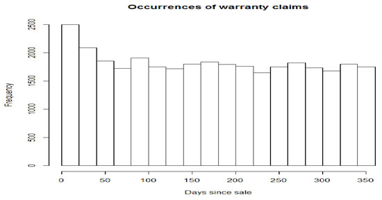
Figure 1.
Histogram of the occurrence times.
Here, we calculate point predictors for with different values of converging towards with these predictive models. For every time , Table 4 presents the LRT results where the last three columns indicate, respectively, the p-values of the k-moment maximum entropy prior with k = 2, 4 and 6 as the null models versus the -moment maximum entropy prior as the alternative models. Note that the last column shows us the number of moments required for our model.
Table 4.
The likelihood ratio test for the automobile warranty claims data sets.
Based on the results in Table 4 with a significance level equal to , we can say that the LRT always rejects the general Poisson–MaxEnt model with the 8-moment prior. Therefore, it supports our model with the 6-moment maximum entropy prior as the adequate prediction model when the maximum entropy prior is used. This means adding other moments does not allow us to reject our 6-moment predictive model; thus, the LRT provides a stopping rule. The only exception occurs when equals 365, where the LRT supports the MaxEnt prior with only 2-moments.
The likelihood ratio test appears to provide an appropriate stopping rule, since its corresponding average discrepancy values (values in bold font) are always very close to the smallest absolute error discrepancies. Furthermore, the most interesting result in Table 5 is that the Poisson MaxEnt model suggested by the LRT always outperforms the NB model.
Table 5.
Absolute error discrepancy of point predictors with different values of for the automobile warranty claims data sets with MLE–MaxEnt estimation method.
Finally, we note from this example that, when , the Poisson–MaxEnt with 2-moments and the NB models are similar in terms of performance. On the other hand, when , the general Poisson–MaxEnt predictive model suggested by the LRT clearly performs better than the classical NB model using the conjugate gamma prior.
5. Conclusions
In this paper, we have outlined a model, the general Poisson–MaxEnt model with the k-moment prior for the prediction problem for the HPPr. The effectiveness of the model for prediction measured by different goodness-of-fit criteria is tested. We note that the use of this prior with more than 2-moments allows us to remove the restriction of Wragg and Dawson that the coefficient of variation must be less than one.
We use maximum likelihood to estimate the parameters in the general Poisson–MaxEnt model because it is computationally less complex than the matching moments procedure when . The k-moment maximum entropy prior produced very good results in terms of the comparison criteria (KL divergence and a discrepancy measure) we used in our simulation studies with different values for the coefficient of variation. Finally, we have illustrated on a data set the effectiveness of the general Poisson–MaxEnt model for prediction problems, when the LRT is used as a stopping rule for adding more moments.
We know that the classical NB model obtained with the conjugate gamma prior is the usual choice for prediction problems. This model can be used whatever the value of coefficient of variation. We have seen by using simulation studies and illustrating the method on a data set that the Poisson–MaxEnt model with has generally a better performance than the NB model whatever the value of coefficient of variation.
In our future research, it will be very interesting to use these methods allowing prediction of recurrent events using more flexible nonhomogeneous Poisson processes with priors that have heavy tails and various shapes and with possible heterogeneity amongst the individual units modeled with higher moment maximum entropy priors.
Acknowledgments
The research of the first author was partially supported by a fellowship from Université du Québec à Montréal (UQAM). The research of the second and third authors was partially supported by NSERC of Canada.
Author Contributions
Lotfi Khribi, Brenda MacGibbon and Marc Fredette organized the research. Lotfi Khribi carried out the model calculations. Lotfi Khribi and Brenda MacGibbon wrote the manuscript. Lotfi Khribi, Brenda MacGibbon and Marc Fredette revised the manuscript. All authors have read and approved the final manuscript.
Conflicts of Interest
The authors declare no conflict of interest.
Appendix A. Moment Matching Estimation for the Poisson–MaxEnt Model
Here, we illustrate how to use the moment matching (MM) estimation for the Poisson–MaxEnt method.
We consider the maximum entropy method for the empirical Bayes general Poisson–MaxEnt model with MM. This involves matching the first k unconditional moments with with their corresponding empirical non-central moments.
Letting , we can show that the first k unconditional moments for an unknown parameter truncated at 0 are defined by: ; and, for , we have the following recurrence formula:
Then, we have to solve the following nonlinear system of equations:
with with and ; ; and the following recurrence formula for :
where is the sample average of , while is the sample average of the s.
One way to solve this problem is to transform the nonlinear system of Equation (A1) into an unconstrained optimization problem and then use a numerical integration and the “fminsearchbnd” MATLAB function described earlier to obtain an exact density
Here, we note that [7] has implemented his numerical method in MATLAB, which allows us to estimate the vector of parameters in the maximum entropy distribution.
Another way is to specify the k-moment prior completely. For that, we substitute (A2) into (A1) and solve this highly nonlinear set of equations for the in terms of the k known empirical moments.
For given , , …, , the corresponding values of , , …, are obtained by solving the set nonlinear equations:
We see that this is not an easy problem as it involves, among other things, the integration of an exponential function in which the exponent is of degree k and also that no general analytic solution exists for this highly nonlinear set of equations. This is why we adopt a numerical method that should lead to good approximate solutions for the vector .
Let be a vector of initial values of and let be the vector defined by the equations
By linearizing (A3), we see that the approximately satisfies k simultaneous equations of the form
where
Thus, given a sufficiently good initial approximation , the system (A5) is solved for , which becomes our new vector of trial , and iterations continue until becomes appropriately small.
We note that, for , a numerical calculation with MATLAB has to be performed, but, for recurrence relations of the form
can be used.
References
- Xu, G.; Chiou, S.H.; Huang, C.Y.; Wang, M.C.; Yan, J. Joint scale-change models for recurrent events and failure time. J. Am. Stat. Assoc. 2015, 111, 1–38. [Google Scholar] [CrossRef]
- Brijs, T.; Karlis, D.; Swinnen, G.; Vanhoof, K.; Wets, W.; Manchanda, P. A multivariate Poisson mixture model for marketing applications. Stat. Neerlandica 2004, 58, 322–348. [Google Scholar] [CrossRef]
- Fredette, M.; Lawless, J.F. Finite horizon prediction of recurrent events with application to forecast of warranty claims. Technometrics 2007, 49, 66–80. [Google Scholar] [CrossRef]
- Khribi, L.; Fredette, M.; MacGibbon, B. The Poisson maximum entropy model for homogeneous Poisson processes. Commun. Stat.-Simul. Comput. 2015, 45, 3435–3456. [Google Scholar] [CrossRef]
- Aroian, L.A. The fourth degree exponential distribution function. Ann. Math. Stat. 1948, 19, 589–592. [Google Scholar] [CrossRef]
- Mohammad-Djafari, A. Maximum likelihood estimation of the Lagrange parameters of the maximum entropy distributions. In Maximum Entropy and Bayesian Methods; Smith, C.R., Erickson, G.J., Neudorfer, P.O., Eds.; Kluwer Academic Publishers: Norwell, MA, USA, 1992; Volume 50, pp. 131–139. [Google Scholar]
- Mohammad-Djafari, A. A Matlab program to calculate the maximum entropy distributions. In Maximum Entropy and Bayesian Methods; Smith, C.R., Erickson, G.J., Neudorfer, P.O., Eds.; Kluwer Academic Publishers: Norwell, MA, USA, 1992; Volume 50, pp. 221–233. [Google Scholar]
- Wragg, A.; Dowson, D.C. Fitting continuous probability density functions over (0, ∞) using information theory ideas. IEEE Trans. Inf. Theory 1970, 16, 226–230. [Google Scholar] [CrossRef]
- Wu, X. Calculation of maximum entropy densities with application to income distribution. J. Econom. 2003, 115, 347–354. [Google Scholar] [CrossRef]
- Zellner, A.; Highfield, R.A. Calculation of maximum entropy distributions and approximation of marginal posterior distributions. J. Econom. 1987, 37, 195–209. [Google Scholar] [CrossRef]
- Broadbent, D.E. A difficulity in assessing bimodality in certain distributions. Br. J. Math. Stat. Psychol. 1966, 19, 125–126. [Google Scholar] [CrossRef]
- Eisenberger, I. Genesis of bimodal distributions. Technometrics 1964, 6, 357–363. [Google Scholar] [CrossRef]
- Kullback, S.; Leibler, R.A. On information and sufficiency. Ann. Math. Stat. 1951, 22, 79–86. [Google Scholar] [CrossRef]
- Dick, J.; Pillichshammer, F. Discrepancy Theory and Quasi-Monte Carlo Integration; Springer: New York, NY, USA, 2014. [Google Scholar]
- Shannon, C.E. The mathematical theory of communication. Bell Syst. Tech. J. 1948, 27, 379–423. [Google Scholar] [CrossRef]
- Weinstock, R. Calculus of Variations—With Applications to Physics and Engineering; McGraw-Hill: New York, NY, USA, 1952. [Google Scholar]
- Cook, R.J.; Lawless, J.F. The Statistical Analysis of Recurrent Events; Springer: New York, NY, USA, 2007. [Google Scholar]
- Noel van Erp, H.R.; Linger, R.O.; Van Gelder, P.H.A.J.M. Deriving proper uniform priors for regression coefficients, Parts I, II, and III. Entropy 2017, 19, 250. [Google Scholar]
- Terenin, A.; Draper, D. A Noninformative prior on a space of distribution functions. Entropy 2017, 19, 391. [Google Scholar] [CrossRef]
- Lawless, J.F.; Fredette, M. Frequentist prediction intervals and predictive distributions. Biometrika 2005, 92, 529–542. [Google Scholar] [CrossRef]
- Spiegelhalter, D.; Thomas, A.; Best, N.; Lunn, D. WinBUGS User Manual, Version 1.4; Technical Report; Medical Research Council Biostatistics Unit: Cambridge, UK, 2003; Available online: http://www.politicalbubbles.org/bayes_beach/manual14.pdf (accessed on 13 December 2017).
- Talvila, E. Necessary and sufficient conditions for differentiating under the integral sign. Am. Math. Mon. 2001, 108, 544–548. [Google Scholar] [CrossRef]
- Aida, T. Model selection criteria using divergences. Entropy 2014, 16, 2686–2689. [Google Scholar]
- Lods, B.; Pistone, G. Information geometry formalism for the spatially homogeneous boltzmann equation. Entropy 2015, 17, 4323–4363. [Google Scholar] [CrossRef]
- Tiňo, P. Pushing for the extreme: Estimation of Poisson distribution from low count unreplicated data-how close can we get? Entropy 2013, 15, 1202–1220. [Google Scholar] [CrossRef]
- Mead, L.R.; Papanicolaou, N. Maximum entropy in the problem of moments. J. Math. Phys. 1984, 25, 2404–2417. [Google Scholar] [CrossRef]
- Kalbfleisch, J.D.; Lawless, J.F.; Robinson, J. Methods for the analysis and prediction of warranty claims. Technometrics 1991, 33, 273–285. [Google Scholar] [CrossRef]
- Wilks, S.S. The large-sample distribution of the likelihood ratio for testing composite hypotheses. Ann. Math. Stat. 1938, 9, 60–62. [Google Scholar] [CrossRef]
© 2017 by the authors. Licensee MDPI, Basel, Switzerland. This article is an open access article distributed under the terms and conditions of the Creative Commons Attribution (CC BY) license (http://creativecommons.org/licenses/by/4.0/).