Abstract
We study spatial scaling and complexity properties of Amazonian radar rainfall fields using the Beta-Lognormal Model (BL-Model) with the aim to characterize and model the process at a broad range of spatial scales. The Generalized Space q-Entropy Function (GSEF), an entropic measure defined as a continuous set of power laws covering a broad range of spatial scales, , is used as a tool to check the ability of the BL-Model to represent observed 2-D radar rainfall fields. In addition, we evaluate the effect of the amount of zeros, the variability of rainfall intensity, the number of bins used to estimate the probability mass function, and the record length on the GSFE estimation. Our results show that: (i) the BL-Model adequately represents the scaling properties of the q-entropy, , for Amazonian rainfall fields across a range of spatial scales from 2 km to 64 km; (ii) the q-entropy in rainfall fields can be characterized by a non-additivity value, , at which rainfall reaches a maximum scaling exponent, ; (iii) the maximum scaling exponent is directly related to the amount of zeros in rainfall fields and is not sensitive to either the number of bins to estimate the probability mass function or the variability of rainfall intensity; and (iv) for small-samples, the GSEF of rainfall fields may incur in considerable bias. Finally, for synthetic 2-D rainfall fields from the BL-Model, we look for a connection between intermittency using a metric based on generalized Hurst exponents, , and the non-extensive order (q-order) of a system, , which relates to the GSEF. Our results do not exhibit evidence of such relationship.
1. Introduction
1.1. Statistical Scaling and Multiplicative Random Cascades
Statistical scaling has provided a rich framework to understand and model the spatiotemporal dynamics and the complexity and intermitency of rainfall fields, including (multi-)fractal, multiscaling, and random cascade models [1,2,3,4,5,6,7,8,9,10,11,12,13,14,15,16,17,18,19].
The strong variability and intermittence of convective tropical rainfall constitute an adequate setting to study the scaling characteristics of rainfall in a wide range of spatio-temporal scales [19,20,21,22,23,24,25,26,27,28,29,30,31]. In particular, Ref. [19] found that 2-D rainfall fields over Amazonia exhibit multiscaling properties in space, which means that the relationship exhibits a non-linear behavior, where is the spatial scale, r the order of the statistical moment and is the r-th moment scaling exponent. Additionally, they show that both the diurnal cycle and the predominant atmospheric regime of Amazonian rainfall (Easterly or Westerly) exert a strong control on the scaling properties of Amazonian storms, thus shedding light towards understanding the linkages between scaling statistics and physical features of Amazonian rainfall fields.
1.2. Multiplicative Random Cascades and the Beta-LogNormal Model
The Beta-Lognormal Model (hereafter BL-Model) is a discrete 2-D random cascade non-Markovian model [13] based on the observed scaling properties of rainfall, with only two parameters: denoting the variability of rainfall intensity, and representing the rainy area fraction. This model provides a framework to carry out numerical experiments controlling features of rainfall (e.g., and ), but also to link diverse statistical and physical characteristics across spatial scales (e.g., Refs. [19,31] and Section 1.5, respectively). In addition, the model provides a tool to investigate the robustness and sensitivity of statistical metrics to poor sampling, data sparsity and intermittency of high-resolution 2-D rainfall fields.
The construction of a spatially distributed discrete random cascade model usually begins with a given mass (or volume) of rainfall over a two-dimensional () bounded region [6]. The region is successively divided into b equal parts () at each step, and during each iteration the mass obtained at the previous step is distributed into the b subdivisions through multiplication by a set of “cascade generator” W, as shown schematically in Figure 1 (for the case of and ). If the initial area (at level 0) is assigned an average intensity , this gives an initial volume , where is the outer length scale of the study area. Thus, at the first level the volume is subdivided into subareas denoted by , . At the second level, each of the previous subareas is further subdivided into subareas, which are denoted by , i = 1, 2, ..., 16, for a total of subareas. This subdivision is continued further down the spatial scale, leading at the nth level, to subareas denoted by , i = 1, 2, ..., .
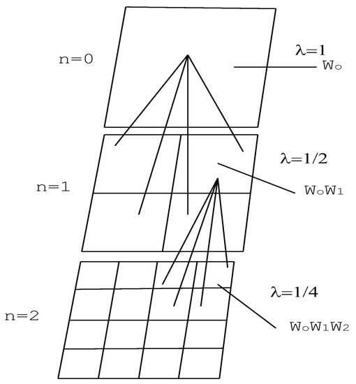
Figure 1.
Schematic plot of the random cascade geometry taken from Gupta and Waymire [33].
As shown in Figure 1, after the first subdivision, the four subareas (, ) are assigned volumes , for . Upon subdivision, the volumes in subareas at the nth subdivision, , i = 1, 2, ..., , are given by,
where, for each cascade’s level j, i represents one subarea belonging to the level. The multipliers W in Equation (1) are non-negative random cascade generators, with to ensure that the mass is conserved on average, from one discretization level to the next one. Over and Gupta [13,32] proposed the so-called BL-Model for the cascade generators W. The BL-Model considers W as a composite generator, , where B is a generator from the “Beta model” and Y is drawn from a Lognormal distribution [33]. Essentially, the Beta model partitions the region into sets with and without rain, while the Lognormal model then assigns a certain amount of rainfall to each rainy area fraction. The Beta model exhibits a discrete probability mass function with just two possible outcomes ( and ), given as
where b is the branching number and is a parameter. Since Y belongs to the Lognormal distribution, it can be expressed as , where X is a standard Normal r.v. and () is a parameter equal to the variance of , with the condition that . In such case, it is easy to show that the condition is also satisfied. The probability distribution function of can thus be expressed as
The parameters of the BL-Model ( and ) can be estimated [13,32] through the so-called Mandelbrot–Kahane–Peyriere (MKP) function [34,35]. The MKP function characterizes the fractal or scale-invariant behavior of the multiplicative cascade process. Over and Gupta [32] theoretically derived an expression for for the BL-Model, in terms of the cascade parameters , , b and exponent r, such that,
Thus, provided that a rainfall field belongs to a discrete random cascade with generators satisfying the BL-Model, the expression given in Equation (5) can be matched with the empirically determined estimators, , to estimate and . The first and second derivatives of with respect to r, the latter of which is given by Equation (5), can be used to obtain [20,32],
Both and can be computed by numerically estimating the derivatives of the empirical slopes of the scaling relation between and r, using the log–log plotting of versus as,
where are the sample moments and is the corresponding scale ratio. Equations (6) and (7) are combined together to express the cascade parameters and in terms of and as follows:
1.3. q-Entropy
There is a wide family of generalized entropic functions with various degrees of sophistication in the literature [36,37,38,39,40]. In particular, Tsallis [40] proposed the concept of nonadditive entropy (hereafter q-entropy), which has shown to be useful in the study of a broad range of phenomena across diverse disciplines [41,42], related to the well known Rényi entropy [43]. The q-entropy is defined as,
which, in the limit , recovers the usual Boltzmann–Gibbs–Shannon entropy, S [44], which is additive; in other words, for a system composed of any two (probabilistically) independent subsystems, the entropy S of the sum is the sum of their entropies [45], such that, if A and B are independent,
It turns out that Tsallis entropy, (), violates this property, and is therefore nonadditive. Thus, the additivity depends on the functional form of the entropy in terms of probabilities [45]. Therefore, if A and B are independent, then
More generally, if A and B are not probabilistically independent then,
Taking the words of Tsallis [45], the value of q is useful to characterize the universal classes of nonadditivity. He argues that it is determined a priori by the microscopic dynamics of the system, which means that the thermostatistical entropy is not universal but depends on the system or, more precisely, on the non-additive universality class to which the system belongs. It is worth mentioning the difference between additivity and extensivity, which is clearly explained in [45], as follows:
“An entropy of a system or of a subsystem is said extensive if, for a large number N of its elements (probabilistically independent or not), the entropy is (asymptotically) proportional to N. Otherwise, it is nonextensive. This means that extensivity depends on both the mathematical form of the entropic functional and the possible correlations existing between the elements of the system. Consequently, for a (sub)system whose elements are either independent or weakly correlated, the additive entropy S is extensive, whereas the nonadditive entropy () is nonextensive. In contrast, however, for a (sub)system whose elements are generically strongly correlated, the additive entropy S can be nonextensive, whereas the nonadditive entropy () can be extensive for a special value of q.”
Additionally, recent studies [28,30,31] have investigated the relationship between the q-entropy and the Generalized Pareto distribution (which is relevant in hydrological analysis). In particular, the maximization of the q-entropy under a prescribed mean leads to a Pareto probability distribution with power-law tail [28,46,47,48], which belongs to the family of Lévy stable distributions [49], specifically to Type II Generalized Pareto distributions. For , the original distribution takes the form of the Zipf–Mandelbrot type [50,51,52], which decays as a power law for large values of x, and all moments are divergent when [53].
As such, the q-entropy constitutes a useful tool for the characterization of rainfall, and at the same time motivates interesting discussions about the physical interpretation of entropic non-linear metrics, their connection with stochastic processes (Multiplicative Cascades), and allows revisiting its applicability in geosciences (see Section 5).
1.4. Generalized Space-Time q-Entropy in Rainfall Data
Previous studies [28,30,31] introduced the Generalized Space-Time q-Entropy as a new method to study the organization degree and the scaling properties of rainfall, by considering the space-time structure of rainfall as a system conformed by correlated subsystems, which is evident in the hierarchical structure of convective rainfall. The time generalized q-entropy is defined as a function of order, q, and aggregation interval, T, as [28]:
where q is the statistical order and is the probability of occurrence of at aggregation interval, T. Ever since the original work [28], different characteristics of the Space and Time Generalized q-entropy of rainfall were reported later on [30,31], such as:
- decreases monotonically with q for all values of T.
- For a given value of q, estimates are inversely related to T for , but directly related for .
- Estimates of recover the standard entropy for different values of T.
- Estimates of increase with T for values of , up to a certain saturation value (maximum q-entropy).
- The function vs. T in log–log space, for different values of q, can be considered an (time) entropy analogous of the (space) structure function in turbulence [54].
- The scaling exponents, , or the slope of the relation vs. T in log–log space, for different values of q, exhibit a non-linear growth with q, such that for . This result allowed extending the conclusions from the standard Shannon entropy to the generalized q-entropy.
- The scaling exponents of saturation, , are different in time and space for hydrological data, such as time series of rainfall, for which , for time series of streamflows, for which , and for the spatial analysis of radar rainfall fields in Amazonia, for which .
Analogous to Equation (15), the Space Generalized q-Entropy was introduced by [31], to study 2-D rainfall fields, using as the spatial scale, and the probability of occurrence of associated with , such that
With the aim of linking the present study with the previous ones, some important results are worth mentioning:
- Poveda [28] studied the time scaling properties of tropical rainfall in the Andes of Colombia upon temporal aggregation and introduced the Generalized Time q-Entropy Function (GTEF), as a time analogous for q-entropy of the structure function in turbulence [54]. He showed that the scaling exponents, of the relation vs. T in log–log space, for different values of q, exhibit a non-linear growth with q up to for , putting forward the conjecture that the time dependent q-entropy, with , for .
- Salas and Poveda [30] revisited results reported in [28], and analyzed the time scaling properties of Shannon’s entropy for the same data set in terms of the sensitivity to the record length, and the effect of zeros in rainfall data, and proposed the GTEF to study the scaling properties of river flows. They highlighted two important results: (i) The scaling characteristics of Shannon’s entropy differ between rainfall and streamflows owing to the presence of zeros in rainfall series; and (ii) the GTEF exhibits multi-scaling for rainfall and streamflows. For rainfall, the relation vs. T in log–log space for different values of q, exhibits a non-linear growth with q, up to for , in contrast to the scaling properties of river flows which exhibit a non-linear growth with q, up to for .
- Poveda and Salas [31] studied diverse topics such as statistical scaling, Shannon entropy and Space-Time Generalized q-Entropy of Mesoscale Convective Systems (MCS) as seen by the Tropical Rainfall Measuring Mission (TRMM) over continental and oceanic regions of tropical South America, and in Amazonian radar rainfall fields. The main result of their study is that both the GTEF and GSEF exhibit linear growth in the range , and saturation of the exponent for , but for the spatial analysis (GSEF) the exponent tappers off at 1.0, whereas for the temporal analysis (GTEF) the exponent saturates at 0.5. In addition, results are similar for time series extracted from radar rainfall fields in Amazonia (radar S-POL) and in-situ rainfall series in the tropical Andes.
1.5. Easterly and Westerly Regimes of Amazonian Rainfall
The WETAMC/LBA campaign (January–February 1999) found that wet-season convection in Amazonia exhibits two general modes, hereinafter, the Westerly and Easterly regimes [55], which are highly correlated to changes in the 850–700 hPa zonal wind direction [56]. According to data from the NCEP-NCAR Reanalysis, as well as from the Fazenda Nossa Senhora radiosonde, the Easterly (negative values) and Westerly (positive) regimes are clearly differentiated in both data sets [19,31]. Furthermore, radar observations from southwestern Amazonia during TRMM-LBA suggest that there was relatively little difference in the daily mean rainfall totals between Easterly and Westerly regimes [57]. In addition, the TRMM-LBA and TRMM satellite observations suggested marked differences in rainfall rate distributions, with the Easterly regime (Altiplano/southern Brazil) associated with a broader rain-rate distribution and greater instantaneous rainfall rates [56]. Precipitation features during both regimes can be summarized considering that during the Easterly regime atmospheric conditions are relatively dry, with increased lightning activity and more intense and deeper convective systems. In contrast, the Westerly regime is characterized by a diminished lightning activity, less deep convection and less intense precipitation rates [56,58,59]. The regime associated with stronger vertical development, more lightning activity, and larger instantaneous rainfall rates must be associated with a more “concentrated” daily latent heat release. In addition, two mechanisms have been proposed to explain the observed changes in the overall convective structure and lightning frequency between the two regimes, these mechanisms are tied to either thermodynamics (changes in CAPE and CIN that modify the energetics of the cloud ensemble), or aerosol loading (e.g., changes in cloud condensation nuclei (CCN) concentration that modify microphysical structure of the cloud ensemble) [56].
The aforementioned results have important practical implications in the spatial and temporal scaling features of rainfall fields [28,30,31] although the connections between entropic and scaling statistics with physical characteristics remain elusive. Furthermore, the effect of the space-time structure of rainfall in the scaling of the q-Entropy as well as its sensitivity to the number of bins and to the variability of rainfall intensity and the sample-size must be investigated in depth. Therefore, in the present study, we aim to investigate how the spatial scaling and complexity of rainfall is reflected in different entropic scaling measures within the frameworks of information theory and non-extensive statistical mechanics. The rationale and objectives of this work are presented next.
1.6. Rationale and Objectives
The objectives of our study are based upon the following considerations:
- The presence of zeros in high resolution rainfall records constitute highly important information to understand, diagnose and forecast the dynamics of rainfall [28,60,61]. Salas and Poveda [30] argued that zeros (inter-storm periods) in time series of tropical convective rainfall are associated with the timescale required by nature to build up the dynamic and thermodynamic conditions of the next storm, as an atmospheric analogous of the time of energy build-up between earthquakes, avalanches and many other relaxational processes in nature [62]. Therefore, the role of zeros and their effect on scaling statistics must be investigated to further understand and model high resolution rainfall.
- The aforementioned previous works [28,30,31] are based on available rainfall data (S-POL radar, TRMM satellite and rain gauges), and it is difficult to understand differences of the q-statistics in temporal and spatial scales due to factors such as the intermittency of rainfall, record length, space-time resolution of data sets, and geographic setting.
- The number of bins in the probability mass function constitutes a central issue to quantify entropic measures. Previous studies have shown that the scaling exponent of Shannon entropy under aggregation in time it is not sensitive to either the number of bins [28] or record length [30]. Then, it is necessary to study the sensitivity of the q-entropic measures in order to check their robustness to characterizing 2-D tropical rainfall fields.
The objectives of this study are manifold. They involve questions based on the previous studies [28,30,31], and new ones regarding the entropic scaling measures of rainfall. The objectives of our study are thus:
- To test theBL-Model [13] for 2-D Amazonian rainfall fields considering the Easterly and Westerly climatic regimes [55,56], and using the Generalized Space q-Entropy [31].
- To examine how the spatial structure of rainfall is reflected in the q-entropic scaling measures using the BL-Model and considering the influence of zeros in the GSEF through Montecarlo experiments, aimed at understanding the saturation of the exponent reported by [28,30,31].
- To investigate the connection between parameters of the BL-Model [13] and Amazonian rainfall fields considering the identified climatic regimes [55,56].
- To quantify the sensitivity of the q-entropic scaling statistics to the number of bins and to the variability of rainfall intensity, in an attempt to check the robustness of such statistical tools in the multi-scale characterization of rainfall.
- To link two important theoretical frameworks, namely stochastic processes (Multiplicative Cascades) and Information Theory (non-extensive statistical mechanics), to advance our understanding about the scaling properties of tropical rainfall.
The paper is organized as follows. Section 2 describes the study region and data set. Section 3 discusses the methods employed. Section 4 provides an in-depth discussion of results. Section 5 provides a brief discussion about the criteria and conditions to estimate entropy in geophysical data. Finally, Section 6 contains the conclusions.
2. Study Region and Data Sets
General Information
We use a set of 2-D radar rainfall fields gathered in Amazonia during the January–February 1999 Wet Season Atmospheric Meso-scale Campaign/LBA (WETAMC/LBA), which was designed to study the dynamical, microphysical, electrical, and diabatic heating characteristics of tropical convection over southwestern Amazonia [19,59,63,64]. The WETAMC campaign was developed in the state of Rondônia (Brazil). The data set used in the present study consists on radar scans of storm intensities recorded by the S-POL radar (S-band, dual polarimetric) located at 61.9982 W, 11.2213 S. Data consist of 2 km resolution microwave band reflectivity which is directly related to rainfall intensity, over a circle of ∼31,000 km. Scans produced by the Colorado State University Radar Meteorology Group were available every 7–10 min at the URL http://radarmet.atmos.colostate.edu/trmm-lba/rainlba.html.
Additionally, information about zonal wind velocity at 700 hPa during the study period was obtained from the NCEP/NCAR Reanalysis [65], over the region inside 61 W to 62.8 W and 10.4 S to 12.1 S, corresponding to the area covered by the S-POL radar. Data were obtained 4 times per day at 0000, 0600, 1200 and 1800 LST. In addition, radiosonde data (62.37 W, 10.75 S) were used from the WETAMC campaign in Ouro Preto d’Oeste at the Fazenda Nossa Senhora site, located inside the S-POL radar coverage region. Radiosonde data were obtained in the URL http://www.master.iag.usp.br/lba/.
3. Methods
A set of experiments were developed to study the sensitivity of the GSEF of 2-D Amazonian rainfall fields attempting to link the spatial structure of rainfall and the emerging scaling exponents of the q-entropic analysis [28,30]. To that aim we use the BL-Model proposed by [13] to generate 2-D rainfall fields as a multiplicative random cascade, by varying the model parameters and . A detailed description of each experiment is presented below.
3.1. Parameters of the BL-Model and Amazonian Precipitation Features
The first experiment is carried out by controlling the percentage of wet (rainy) and dray (non-rainy) areas, and the second one by controlling the average intensity of the rainfall field. A set of 1000 simulations for each parameter were carried out. The mass of rainfall over a two-dimensional () region was considered the unit, the branching number for 2-D cascades, and the level of subdivision (see Figure 1) during all experiments, consistently with the observed scans from S-POL radar which are 64 rows × 64 columns matrices ( values). On the other hand, with the aim to link the numerical results from the BL-Model with the S-POL observations, we compared the samples of the estimated cascade’s parameters (Equations (9) and (10)) considering vs. and, vs. using the k-sample tests based on the likelihood ratio [66], which are more robust than traditional methods (e.g., Kolmogorov–Smirnov, Cramer–von Mises, and Anderson–Darling), but also because the climatic regimes prevailing in the study region are statistically different in terms of the continental-scale flow and lightning activity, as well as in the vertical structure of convection and other precipitation features [56].
3.2. Bin-Counting Methods and Entropic Estimators
The correct estimation of diverse informational entropy statistical parameters require to take into account diverse practical considerations. Gong and others [67] argue that there are four practical problems in the estimation of entropy using hydrologic data: (i) the zero effect; (ii) the widely used bin-counting method for estimation of PDFs; (iii) the measure effect; and (iv) the skewness effect. We focus our attention on the second practical issue within the framework of scaling theory using Shannon theoretical entropy inequality [68],
where is the variance of the process at aggregation interval T, with the equality holding just for the for the Gaussian distribution. We use a set of parametric and non-parametric bin-counting methods, such as those introduced by Sturges [69], Dixon and Kronmal [70], Scott [71], Freedman and Diaconis [72], Knuth [73,74], Shimazaki and Shinomoto [75,76], and a recent method for estimating entropy in hydrologic data proposed by Gong et al. [67]. In work, we use common techniques reported in the literature, although there are other methods [77]. Finally, we discuss the effect of the number of bins on the scaling of q-entropy in rainfall fields [28,30,31].
3.3. Sample-Size and Entropy Estimators
Information-theory statistics require an adequate sample size for a proper estimation and interpretation. In spite of the existence of a large body of literature dealing with the problem of estimation of distributions for data sparsity and poor sampling [78,79], the problem constitutes a challenge in geosciences. A recent study on the estimation of Shannon entropy in hydrological records under small-samples [80], employed three different estimators: (i) maximum likelihood (ML); (ii) Chao–Shen (CS); and (iii) James–Stein-type shrinkage (JSS). Their results exhibited that the ML estimator had the worst performance of the three methods, with the largest Mean Squared Errors (MSE) for all sample sizes. In particular, when sample sizes are small (less than 200 data points), the entropy estimator was dramatically underestimated, although errors turned out to decrease quickly when sample sizes increased. Furthermore, when the sample size was larger than 100 data points, the accuracy of the CS and JSS estimators were basically the same, with MSE nearly equal to zero. It is worth mentioning that the said study [80] did not deal either with the effect of the number of bins or the role of zeros in the estimation of entropy.
At the root of the problem of the numerical estimation of entropy, is the sample-size necessary for adequately estimating the underlying probability mass function (pmf) of the process. For example, it is well known that, for the ML estimators, the larger the sample size, the better the estimates will be. In addition, high temporal resolution precipitation data sets (e.g., minutes or hours) are mostly (approximately 90%) constituted by zeros [30], which it is not the case for low-resolution data (e.g., months or years), so an adequate characterization of the tails of the Probability Distribution Function (PDF) requires longer data sets for high-resolution rainfall data than for low-resolution.
With the aim of studying the influence of sample-size in the GSEF, we will compare the q-entropy of the S-POL radar fields (matrices with 64 rows and 64 columns) and synthetic 2-D fields of the BL-Model at different cascade levels, n, to obtain fields with different sizes, , e.g., the cascade level means a 2 × 2 field, (2 rows and 2 columns) and, consequently, a cascade level means a 128 × 128 field. In other words, a field of the BL-Model with has a sample-size and a field of the BL-Model with has a sample-size . Using the synthetic fields, we quantify the q-entropy: (i) estimating the pmf for all the values in the synthetic rainfall field (including zeros); (ii) separing values in two subsets ; and (iii) the minimal quantity of non-zero values in the fields, to ensure robustness in the estimation of . Our results are discussed in Section 4.5.
3.4. Intermittency and q-Order
High space-time resolution tropical rainfall is a highly complex and intermittent process. To analyze its intermittent behavior, several techniques have been proposed in the literature such as: spectral scale invariance analysis [31,81,82,83,84]; moment-scaling analysis [1,3,18,19,31,32,84], and intermittency exponents [84,85]. In this sense, the Generalized Space q-Entropy Function (GSEF) (Section 1.4) can be thought as a measure of (multi-) fractal behavior of a process [30,31]. In addition, the BL-Model (Section 1.2) is directly related to the Mandelbrot-Kahane-Peyriere (MKP) function [34,35] characterizing the fractal (or scale-invariant) behavior of a multiplicative cascade process. Therefore, an interesting question arises: is there any relationship between the GSEF and intermittency estimators? In order to shed light about such question, the BL-Model is used to estimate the q-order, , and the multifractality measure, , defined by Bickel [86], Equation (22).
First, we carry out an experiment for high-resolution-spatial rainfall based on Bickel [86], who showed the relationship between intermittency (multifractality) and the non-extensive order (hereafter q-order) for point processes of dimension D ranging from 0.1 to 0.9. The order in a system is defined in terms of its distance from equilibrium, so the higher disordered, the closer to the equilibrium state. The q-order can be defined as,
where is the q-entropy (Equation (11)) and is the maximum possible value of for the equilibrium condition, which probabilistically can be denoted as for all , whose can be written as,
At this point, it is necessary to emphasize that Equation (19) is a generalization for the extensive order defined as a measure of complexity using the Boltzman-Gibbs-Shannon entropy [87]. In addition, the non-extensive order satisfies with if and if , given any integer l between 1 and N [86,88].
Second, a generalization for , at multiple spatial or temporal scales, is possible using a similar procedure to Equation (15). Therefore, if the spatial scale is denoted as , and the maximum possible value of q-entropy at each scale as , the q-order can be rewritten as,
From previous studies [30,31], it is easy to note that but for the scaling laws and , the scaling exponents are exactly the same, which means that GSEF, , does not change under such transformation.
Third, considering that a process exhibiting a multifractal spectrum whose spectrum of generalized Hurst exponents, , is defined as [86],
which holds for some range T with non-extensive parameter q. For is the mean (first moment) of the absolute displacement and for is the standard deviation of this displacement. Therefore, the intermittency of a nonstationary process can be quantified by its multifractality, , as the difference between two generalized Hurst exponents,
normalized such that for nondegenerate processes, with for monofractals [89].
From previously mentioned considerations, the generalized Hurst exponents for 2-D rainfall fields can be computed as suggested by Carbone [90] in combination with the Equation (21) as follows,
where , and are the number of rows and columns, respectively. The estimates and for , with and such that and exhibit linear relationship with . Then, and are the slopes of the least-square regressions of vs. and vs. , respectively. Finally, the multifractality is estimated as,
In this work, we explore the relationship between intermittency (multifractality), , and q-order, , for synthetic rainfall fields from the BL-Model. The results will be discussed in Section 4.6.
4. Results
4.1. Linking Parameters of the BL-Model with Precipitation Features
Following previous studies [19,31], we classify the available information from the S-POL radar considering the Easterly (negative values) and Westerly (positive) climatic regimes. Then, for both climate regimes, we estimate the parameters of the BL-Model using Equations (9) and (10). Subsequently, we estimate the pmf (histograms) and the Cumulative Distribution Functions (CDFs) of the parameters and (Figure 2 and Figure 3). Results show that the histograms of and are statistically different for both climatic regimes, and, additionally, that the CDFs of the parameter for the Easterly and Westerly regimes are significantly different according to a k-sample test, based on the likelihood ratio [66] at 95% confidence level, but no so for the parameter .
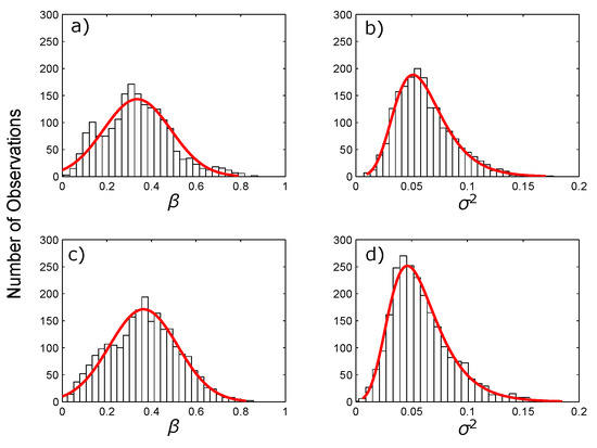
Figure 2.
Histograms for Beta-Lognormal Model parameters in rainfall scans of the S-POL radar: (a,b) Westerly events; and (c,d) Easterly events. (red) the Gaussian function for and the Generalized Extreme Value function for .
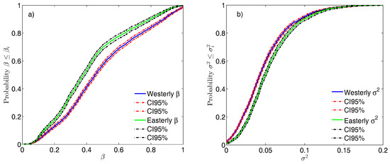
Figure 3.
Empirical Cumulative Distribution Functions for cascade parameters: (a); and (b) using 4227 scans of the S-POL radar considering climatic regimes of Amazonia (1867 scans for Westerly and 2360 for Easterly). The figure shows the confidence bounds using Greenwood’s formula.
Secondly, we estimated the GSEF using a set of 1000 synthetic rainfall fields generated with the average values of and from the S-POL scans (see Figure 4). Figure 5b shows the GSEF of rainfall fields generated using the BL-Model, and the average of the observed S-POL rainfall fields. In addition, Figure 6a shows that the scaling exponents of the GSEF, -observed vs. -simulated, exhibit a very good fit. Furthermore, Figure 6b shows that the BL-Model represents adequately the relationship , with saturation for and . However, observed and simulated rainfall fields exhibit significant differences in the interval ; the S-POL scans do not exhibit power-laws for , albeit in this interval the model shows power-laws with .
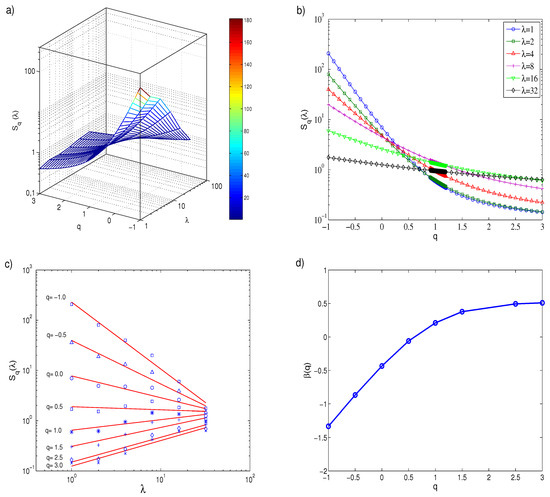
Figure 4.
Space Generalized q-Entropy for the S-POL radar scan 01/10/1999 18:23:15 LST: (a) 3D plot of the Tsallis’ entropy, , for different scale factors, , and q-values from −1.0 to 3.0; (b) projection of S(q,) vs. q for different values of ; (c) projection of S(q,) vs. , for different values of q, or spatial structure function for entropy; and (d) values of the regression slopes of the spatial structure function for entropy, , as function of q, exhibiting a non-linear growth up to for .
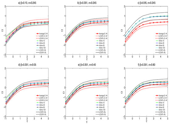
Figure 5.
Space Generalized q-Entropy Function for spatially distribute rainfall as a random cascade varying cascade’s parameters and for 1000 simulated independently fields including zeros in the histogram. and are the lower and upper confidence intervals for Easterly and Westerly events (E-W) and the BL-Model model (BL): (a–c) varying the cascade’s parameter ; and (d–f) varying the cascade’s parameter . In all cases, varying the number of bins (nbins = 10, 30, 50 and 100).
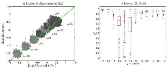
Figure 6.
Validation of the BL-Model using Generalized Space q-Entropy: (a) comparison -Observed vs. -Simulated, (Solid line) relation 1:1; and (b) box plots of the coefficients of determination, , for the power fits from 1000 synthetic fields of BL-Model with and . in the intervals and . The histogram for estimate includes zeros.
Finally, considering that the BL-Model has two parameters, and , it is necessary to link them with precipitation features associated with both climatic regimes in Amazonian rainfall, as follows:
- The cascade parameter, , (Table 1), for the Easterly events is greater than the Westerly events, indicating more spatially concentrated rainfall fields (more zeros in the Easterly scans). This result is related to diverse precipitation features observed during the Easterly regime, given that the atmospheric conditions are relatively dry, with increased lightning activity and more intense and deeper convective systems [56,58,59].
 Table 1. Scans of S-POL radar according to the two identified Amazonian climate regimes.
 - The cascade parameter, , (Table 1), exhibits smaller (larger) values during the Easterly (Westerly) regime, indicating that the variability of rainfall intensity for the Westerly events is higher than for Easterly events. This result is coherent with diverse features observed during the Westerly regime, which is characterized by less lightning activity, less deep convection and less intense precipitation rates [56,58,59].
4.2. The Role of Zeros in the Generalized Space q-Entropy
With the aim of studying the influence of zeros in the estimation of the GSEF, we simulated rainfall fields using the BL-Model with cascade parameters = 0.10, 0.35 and 0.95. In addition, 1000 simulations were carried out for each value of . Modeling a 2-D rainfall field with corresponds to the situation in which the cascade assigns a uniformly distributed unit rainfall intensity over the whole area. In contrast, close to indicates that rainfall is concentrated in a very small area. Our experiments estimate the GSEF for varying values of , while keeping constant and equal to the average value for the Amazonian scans, (see Table 1). Results show that the saturation scaling exponent in the GSEF is significantly affected by the fraction of non-rainy cells (Figure 5a–c). A similar result is found for the minimum value of the scaling exponent in the GSEF, which is significantly increased with the amount of zeros present in the rainfall fields. Figure 7 shows that the scaling exponents and increase with the value of . This behavior is explained by the loss rate of zeros during the change in spatial resolution, as is explained below.
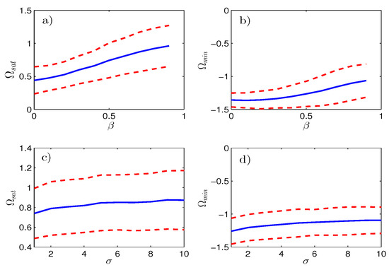
Figure 7.
Sensitivity analysis of the saturation , and minimum scaling exponents in the SGEF for 1000 independent rainfall fields generated by random cascade model [13]. Confidence intervals for in dash line and mean value in solid line. (a) Varying cascade’s parameter and considering = 0.25 constant; (b) varying cascade’s parameter and considering = 0.25 constant; (c) varying cascade’s parameter and considering constant; and (d) varying cascade’s parameter and considering constant.
4.3. The Role of Rainfall Intensity Variability in Generalized Space q-Entropy
The influence of the variability in rainfall intensity on the GSFE was examined with a similar strategy. We generated rainfall fields with cascade parameters = 0.05, 0.40 and 0.80 (1000 simulations for each value), with a constant parameter (see Table 1). Results show that the scaling exponent of saturation, , in the GSEF increases slowly in comparison with the case where the cascade parameter is considered variable. This result implies that the increase or decrease in uncertainty across spatial scales is dominated by the dry areas and not by the variability in rainfall intensity. In general, the scaling exponents and were not affected by changes in (Figure 7c,d). A possible explanation for this result is that the scaling exponents and are directly related to the loss rate of zeros in rainfall fields when data are averaged going from higher resolution (2 km pixel size) to lower resolution scales (32 km pixel size) [30]. Then, if the amount of zeros is constant and the variability of rainfall intensity increases, the loss rate of zeros remains the same regardless of the spatial resolution, which means the scaling exponent is not affected by the cascade parameter .
4.4. Bin-Counting Methods and the Generalized Space q-Entropy
First, we discuss the numerical estimation of Shannon entropy for an i.i.d. Gaussian random variable under increasing aggregation intervals, T, using the analytic inequality given by Equation (17), and the multiple bin-counting methods mentioned in Section 3.2. From that equation, it is easy to see why entropy increases under aggregation of T. The theorem [91] proves that if are i.i.d. random variables, then the expected value , with finite variance . Defining the sum , then the average is , and .
On the other hand, we revisit the classical problem [92] of how and how well diverse information-theoretic quantities, can be estimated given a finite set of i.i.d. r.v., which lies at the heart of the majority of applications of entropy in data analysis. Paninski’s paper focuses on the non-parametric estimation of entropy, and compares different estimation methods without delving into the role of the number of bins. For our proposes, we study the sensitivity of Shannon entropy (Equation (25)) to the number of bins. According to Shannon [44], discrete data entropy can be estimated as,
where represents the probability mass function, such that , and , . Figure 8 shows that the main differences among the different estimation methods are the following:
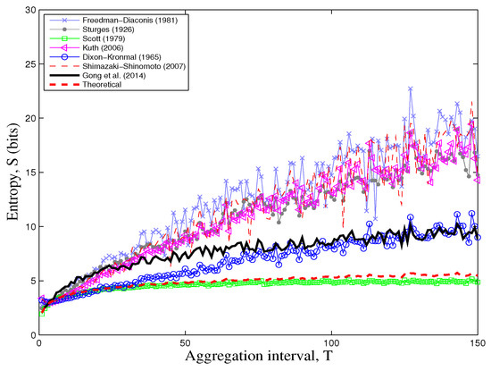
Figure 8.
Numerical estimation of Shannon’s Entropy using multiple bin-counting methods and the theoretical inequality (Equation (17), for a Gaussian r.v. for different levels of aggregation, T).
- The bin-counting method proposed by Dixon and Kronmal [70] is the nearest to the method presented by Gong et al. (2014) for Gaussian r.v. under aggregation, for a number of aggregation intervals greater than 70.
- The theoretical inequality given by Equation (17) is better captured by Scott’s method, although this method shows lower values than the theoretical expression, for aggregation intervals .
- The difference between the theoretical inequality (Equation (17)) and Gong et al.’s [67] method is explained because the “Discrete Entropy” and the “Continuous Entropy” (also referred to as “Differential Entropy”) are related as:where is the discrete entropy with the bin-width and is the corresponding continuous entropy. Thus, the continuous entropy of a r.v. requires to add in the numerical estimation. In our numerical estimation, was selected as the average of the bin-width estimated for the six methods (see the Section 3.2) for each aggregation interval, T, so the behavior of Gong et al.’s method is approximately the average of the set of methods. At this point, it is worth noting that although Gong et al.’s method is designed for hydrological records, it is not free from sensitivity to the number of bins.
- To check the sensitivity of the scaling exponents of the GSEF to the number of bins, we developed a numerical experiment using the BL-Model and 1000 independent simulations for each number of bins n = 10, 30, 50 and 100, with parameters = 0.10, 0.351, and 0.950 and = 0.05, 0.40 and 0.80. Figure 5 and Figure 7 show that the GSEF is not statistically affected either by the number of bins or by the value of when and the sample-size is bigger than 200 data. Consequently, the GSEF is not affect by the bin-counting method.
4.5. Sample-Size and the Generalized Space q-Entropy
We consider 6491 scans of the S-POL radar, each one with 4096 data (64 rows and 64 columns; pixel-size 2 km), of which on average 82% are zeros. Furthermore, approximately 34% of all scans have less than 200 non-zero values. Thus, using the complete data set, the probability mass function (pmf) of some scans could be concentrated in the first bins, with small informational content to the entropic estimator whereas the highest rain values could appear with a very low probability, contributing to augment the entropy. To quantify the effect of sample-size in estimating q-entropy we performed the following experiments:
First, we generated rainfall fields using the BL-Model with constant values of , , in , and the number of bins of the pmf, . Then, we calculated by changing the amount of cascade levels to obtain synthetic rainfall fields with different number of values in the scan (or sample-size) 4, 16, ..., 65,537, and finally we estimated in the following two manners:
- The pmf to calculate was built considering all values in the synthetic rainfall field including zeros.
- The pmf to calculate was built considering all values separated in two subsets: (i) values greater than zero (rain), i.e., ; and (ii) values equal to zero (dry), . For the subset (i), the pmf was built and then corrected by the probability of rainfall () thus, the probability of occurrence of rainfall can be written as .
Figure 9 shows that, in both cases, decreases with sample size, , but the variance of is slightly greater when the pmf was built using all values including zeros (Figure 9a) than when the pmf was built using two separated subsets (Figure 9b). Figure 10 shows that values of q-entropy differ when zeros are included in the pmf and when is calculated separately. Figure 10a shows that values of with zeros in the pmf versus without zeros in the pmf are not significantly different when the sample size (i.e., 64 × 64 matrices or cascade level 6). In contrast, Figure 10b shows that values of with the zeros in pmf versus without the zeros in the pmf are significantly different in fields of sample size (i.e., 256 × 256 matrices or cascade level 8).
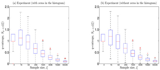
Figure 9.
Boxplots for q-Entropy vs. sample sizes, , in 1000 independent random cascade simulations of the Beta-Lognormal model with parameters and : (a) q-Entropy including zeros in the histogram; and (b) q-Entropy without including zeros in the histogram. In both cases, ().
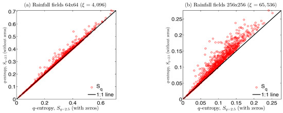
Figure 10.
Comparison of q-Entropy in 1000 independent random cascade fields of the Beta-Lognormal model with parameters and : (a) q-Entropy including zeros in the histogram vs. q-Entropy without zeros in the histogram, cascade’s level , i.e., ; and (b) q-Entropy including zeros in the histogram vs. q-Entropy without zeros in the histogram, cascade’s level , i.e., = 65,536. In both cases, ().
Secondly, we performed a detailed examination of previous results [31] obtained using all the S-POL radar scans, and re-calculated the GSEF varying the sample-size. Results show considerable differences between sample-sizes with less and more than 200 non-zero values. Figure 11 shows differences between the GSEF for all S-POL scans, and the GSEF considering only scans with more than 200 non-zero values, but including zeros in the pmf. Furthermore, Figure 12 shows that the power laws , considering the two climate regimes in Amazonian rainfall, exhibit in the intervals and . For scans with more than 200 non-zero values, the scaling exponents of the relation vs. exhibit a non-linear growth with q, up to for , while in our previous study [31], the GSEF exhibited a non-linear growth with q, up to for .
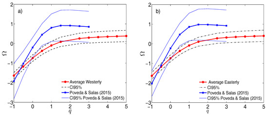
Figure 11.
Space Generalized q-Entropy Functions (SGEFs) for the climate regimes of Amazonian rainfall from the S-POL radar: (a) Westerly events; and (b) Easterly events. (circles) Average SGEF for scans with more than 200 values greater than zero, (dashed lines) confidence intervals (CI); (squares) average SGEF for all the scans available of each climate regime; (solid lines) confidence intervals (CI).
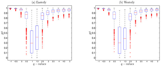
Figure 12.
Coefficient of Determination, , for the power fits from scans radars of the climate regimes in Amazonian rainfall. in the intervals and . The histogram for estimate includes zeros: (a) Easterly events; and (b) Westerly events.
These results turned out to be even more interesting with respect to those presented by [31] for the Generalized Time q-Entropy Function (GTEF) in Amazonian rainfall, whose scaling exponents of the relation vs. T in log–log space, exhibit a non-linear growth with q, up to for . A thorough analysis showed that for the 400 time-series of the S-POL radar used by [31], only the had less than 800 non-zero values, and that the 99% of the time-series had more than 200 non-zero values. Additionally, the scaling exponent of saturation, , for the GTEF remains the same, as well as the q-value for saturation. Therefore, our results suggest that the scaling exponent of across a range of scales in space and time reaches the same maximum value , but the non-additive q value of saturation differs between space scaling () and time scaling (). According to Tsallis [45], these results reflect the differences between the space and time dynamics of the system, although their connection with the physics of rainfall is an open problem.
4.6. Rainfall Intermittency and q-Order
As mentioned in Section 3.4, Bickel [86] showed a positive correlation between multifractality, , and q-order, , for point process with dimension D ranging from 0.1 to 0.9. In this study, we looked for an analogous relationship for synthetic 2-D rainfall fields from the BL-Model. Our results show that for vs. k and vs. k, both cases exhibit linear relationship in the log–log graph to estimate the generalized Hurst exponents and and subsequently as we explained in Section 3.4. Figure 13 shows a typical regression for a synthetic rainfall field created with the BL-Model with and , with average intermittency . However, there is no evidence of a clear-cut relationship between and in our numerical experiments (figures not shown here). Those results can be explained because the point-process model used by Bickel [86] is a Markovian model whose stochastic properties and probability distribution function (PDF) differ from point-process models for rainfall [93,94], which do not explicitly consider statistical scaling properties [95]. In addition, the BL-Model is a non-Markovian rainfall model based on the spatial statistical (multi) scaling properties, whose PDF is well known across spatial scales emerging as power laws, . The study of the linkages between intermittency and q-entropic statistics are outside the scope of this work that deserves to be explored in detail in future works.
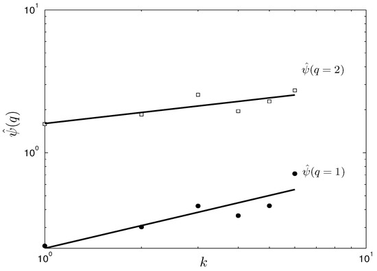
Figure 13.
Typical least-square regressions and with and , for a synthetic 2-D rainfall field from the BL-Model with , and cascade level .
5. Discussion
In spite of the increasing interest in entropic techniques in geosciences, few studies have discussed diverse underlying assumptions regarding the data to guarantee their applicability. In the case studied, high-resolution rainfall records are neither i.i.d. nor with continuous pdf, so the appropriate estimation of entropy needs clarity on the implicit assumptions in data analysis.
First, the i.i.d. condition for rainfall is not satisfied because: (i) the spatial dynamics of mesoscale rainfall has strong spatial correlations [33] (e.g., for Amazonian rainfall see [31]); and (ii) the temporal dynamics of tropical rainfall reflects long-term correlations [28] (see Figure 14). However, by definition, q-entropy, , for , considers probabilistically dependent subsystems, with non-negligible global correlations, whereas Shannon entropy (, for ) considers probabilistically independent subsystems [45,96]. Hence, the non-i.i.d. nature of data is not a restriction in the framework of non-extensive entropy, whereas in the framework of extensive entropy such non-i.i.d nature must be used under specific assumptions (e.g., for weakly correlated sub-systems).
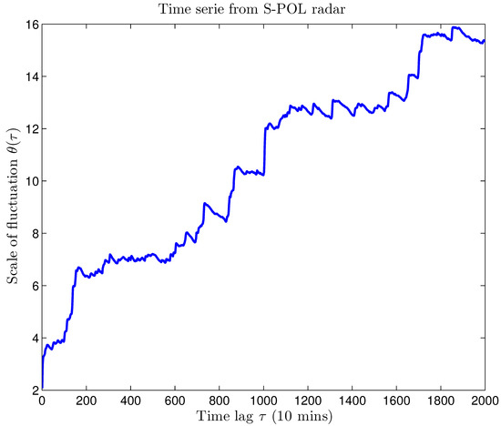
Figure 14.
Scale of fluctuation, , for a time serie of Amazonian rainfall from S-POL radar.
Second, high-resolution Amazonian rainfall records do not satisfy the condition of continuous pdf because zeros constitute more than 80% of data in spatiotemporal scales. Therefore, although continuity in pdf is a fundamental requirement to estimate the additive (Shannon) entropy using the most common estimators [77,97], the condition of pdf’s continuity for q-entropy is not clear in the literature. This is a relevant topic for further research.
Finally, an alternative option to deal with the conditions behind entropic estimators consists in finding a transformation that generates i.i.d data exhibiting a continuous pdf. However, that transformation constitutes a great challenge in geosciences, more so having in mind that such a transformation include multi-scale statistical properties.
6. Conclusions
Using 2-D radar rainfall fields from Amazonia, we investigate the spatial scaling and complexity properties of Amazonian rainfall using the Generalized Space q-Entropy Function (GSEF), defined as a set of continuous power laws covering a broad range of spatial scales, , to test for the validity of the random multiplicative cascade BL-Model in representing 2-D properties of observed rainfall fields. The spatial scaling analysis considered the Westerly and Easterly weather regimes in the Amazon basin. Our results show that for both climate regimes the GSEFs are not statistically different whereas the BL-Model parameters and are statistically different.
We tested the skill of the BL-Model in reproducing the space scaling properties of q-entropy reported in previous works. Our results evidence that the BL-Model appropriately reproduces the relationship , with saturation for and . Furthermore, the power laws, , observed in S-POL rainfall scans exhibit in the intervals and , whereas synthetic rainfall fields generated with the BL-Model exhibit power laws in the intervals and . This result evidences that the q-entropy allows to successfully characterizing the spatial scaling properties of high resolution Amazonian rainfall, thus confirming the validity of this tool in the study of systems conformed by strongly correlated subsystems, for which the Shannon entropy () is no longer valid. In particular, the spatial scaling structure of Amazonian rainfall can be characterized by a non-additivity value, , at which rainfall reaches its the maximum scaling exponent .
Using Montecarlo experiments with the BL-Model, we studied the influence of zeros and rainfall intensity on the estimation of the GSEF, aiming to explain the differences of the saturation exponent found between multiple data sets used in previous works [30,31]. Our results evidence that: (i) the scaling exponent of saturation is related to the non-rainy area fraction, represented by ; and (ii) the variability in rainfall intensity, represented by , does not affect significantly the GSEF. Then, changes in saturation of the scaling exponent are related to the intermittence properties of high-resolution rainfall.
In addition, we studied the influence of bin-counting methods and sample-size in the estimation of entropy and q-entropy. We used a set of parametric and non-parametric bin-counting methods showing the difficulties in estimating Shannon entropy with the well-known inequality linking variance and entropy for Gaussian i.i.d. random variables. Furthermore, we explored the sensitivity of the GSEF to the number of bins (nbins). Our results evidenced that the GSEF is a robust measure provided . On the other hand, we performed a detailed examination of the results by Poveda and Salas [31] to check the influence of the sample-size, , in the estimation of the q-entropy. We studied synthetic 2-D fields of the BL-Model from 2 × 2 (rows and columns) to 128 × 128 (rows and columns) quantifying the q-entropy with respect to: (i) all values inside the rainfall fields (including zeros) in the probability mass function (pmf); (ii) pmf considering ; and (iii) the minimum amount of non-zero values inside the rainfall fields. Our results evidenced that for small-samples the generalized space q-entropy function may incur in considerable bias, and our experiments showed that a rainfall field requires at least 200 non-zero values so that the estimation of q-entropy be robust.
Finally, we explored a possible relationship between a measure of multifractality and the q-order . Our results suggest that the relationship found by Bickel [86] could be related to the point process used therein. In our case, for the BL-Model based on multiplicative cascades there is not evidence of such links between and .
Acknowledgments
We thank the Colorado State University Radar Meteorology Group for radar data and the LBA project for providing access to the Fazenda Nossa Senhora radiosonde. The work of H.D.S. is supported by COLCIENCIAS—Call for National Doctorates 617 (2014). The work of G.P. and O.J.M. is supported by Universidad Nacional de Colombia at Medellin.
Author Contributions
H.D.S., G.P. and O.J.M. conceived and designed the study. H.D.S. prepared the data and performed computations and simulations. H.D.S., G.P. and O.J.M. discussed and analyzed the data and results. H.D.S. and G.P. wrote the manuscript.
Conflicts of Interest
The authors declare no conflict of interest.
References
- Deidda, R.; Benzi, R.; Siccardi, F. Multifractal modeling of anomalous scaling laws in rainfall. Water Resour. Res. 1999, 35, 1853–1867. [Google Scholar] [CrossRef]
- Devineni, N.; Lall, U.; Xi, C.; Ward, P. Scaling of extreme rainfall areas at a planetary scale. Chaos 2015, 25, 075407. [Google Scholar] [CrossRef] [PubMed]
- Foufoula-Georgiou, E. On scaling theories of space-time rainfall: Some recent results and open problems. In Stochastic Methods in Hydrology: Rainfall, Land Forms and Floods; Barndor-Neilsen, O.E., Gupta, V.K., Pérez-Abreu, V., Waymire, E., Eds.; World Science: Hackensack, NJ, USA, 1998; pp. 25–72. [Google Scholar]
- Gupta, V.K.; Waymire, E. Multiscaling properties of spatial rainfall and river flow distributions. J. Geophys. Res. 1990, 95, 1999–2009. [Google Scholar] [CrossRef]
- Harris, D.; Foufoula-Georgiou, E.; Droegemeier, K.K.; Levit, J.J. Multiscale statistical properties of a high-resolution precipitation forecast. J. Hydrometeorol. 2001, 2, 406–418. [Google Scholar] [CrossRef]
- Jothityangkoon, C.; Sivapalan, M.; Viney, N. Test of a space-time model of daily rainfall in soutwestern Australia based on nonhomogeneous random cascades. Water Resour. Res. 2000, 36, 267–284. [Google Scholar] [CrossRef]
- Gentine, P.; Troy, T.J.; Lintner, B.R.; Findell, K.L. Scaling in Surface Hydrology: Progress and Challenges. J. Contemp. Water Res. Educ. 2012, 147, 28–40. [Google Scholar] [CrossRef]
- Lovejoy, S. Area-perimeter relation for rain and cloud areas. Science 1982, 216, 185–187. [Google Scholar] [CrossRef] [PubMed]
- Lovejoy, S.; Schertzer, D. Multifractal analysis techniques and the rain and cloud fields from 103 to 106 m. In Non-Linear Variability in Geophysics: Scaling and Fractals; Kluwer Academic Publishers: Norwell, MA, USA, 1991; pp. 111–144. [Google Scholar]
- Lovejoy, S.; Schertzer, D. Scale invariance and multifractals in the atmosphere. In Encyclopedia of the Environment; Pergamon Press: New York, NY, USA, 1993; pp. 527–532. [Google Scholar]
- Nordstrom, K.M.; Gupta, V.K. Scaling statistics in a critical, nonlinear physical model of tropical oceanic rainfall. Nonlinear Process. Geophys. 2003, 10, 1–13. [Google Scholar] [CrossRef]
- Nykanen, D.K. Linkages between orographic forcing and the scaling properties of convective rainfall in mountainous regions. J. Hydrometeorol. 2008, 9, 327–347. [Google Scholar] [CrossRef]
- Over, T.M.; Gupta, V.K. Statistical analysis of mesoscale rainfall: Dependence of a random cascade generator on large-scale forcing. J. Appl. Meteorol. 1994, 33, 1526–1542. [Google Scholar] [CrossRef]
- Perica, S.; Foufoula-Georgiou, E. Linkage of scaling and thermodynamic parameters of rainfall: Results from midlatitude mesoscale convective systems. J. Geophys. Res. 1996, 101, 7431–7448. [Google Scholar] [CrossRef]
- Perica, S.; Foufoula-Georgiou, E. Model for multiscale disagreggation of spatial rainfall based on coupling meteorological and scaling descriptions. J. Geophys. Res. 1996, 101, 26347–26361. [Google Scholar] [CrossRef]
- Singleton, A.; Toumi, R. Super-Clausius-Clapeyron scaling of rainfall in a model squall line. Q. J. R. Meteorol. Soc. 2013, 139, 334–339. [Google Scholar] [CrossRef]
- Yano, J.-I.; Fraedrich, K.; Blender, R. Tropical convective variability as 1/f noise. J. Clim. 2001, 14, 3608–3616. [Google Scholar] [CrossRef]
- Barker, H.W.; Qu, Z.; Bélair, S.; Leroyer, S.; Milbrandt, J.A.; Vaillancourt, P.A. Scaling properties of observed and simulated satellite visible radiances. J. Geophys. Res. Atmos. 2017, 122. [Google Scholar] [CrossRef]
- Morales, J.; Poveda, G. Diurnally driven scaling properties of Amazonian rainfall fields: Fourier spectra and order-q statistical moments. J. Geophys. Res. 2009, 114, D11104. [Google Scholar] [CrossRef]
- Over, T. M. Modeling Space-Time Rainfall at the Mesoscale Using Random Cascades. Ph.D. Thesis, University of Colorado, Boulder, CO, USA, 1995; 249p. [Google Scholar]
- Gorenburg, I.P.; McLaughlin, D.; Entekhabi, D. Scale-recursive assimilation of precipitation data. Adv. Water Resour. 2001, 24, 941–953. [Google Scholar] [CrossRef]
- Bocchiola, D. Use of Scale Recursive Estimation for assimilation of precipitation data from TRMM (PR and TMI) and NEXRAD. Adv. Water Resour. 2007, 30, 2354–2372. [Google Scholar] [CrossRef]
- Lovejoy, S.; Schertzer, D.; Allaire, V.C. The remarkable wide range spatial scaling of TRMM precipitation. Atmos. Res. 2008, 90, 10–32. [Google Scholar] [CrossRef]
- Gebremichael, M.; Over, T.M.; Krajewski, W.F. Comparison of the Scaling Characteristics of Rainfall Derived from Space-Based and Ground-Based Radar Observations. J. Hydrometeorol. 2006, 7, 1277–1294. [Google Scholar] [CrossRef]
- Gebremichael, M.; Krajewski, W.F.; Over, T.M.; Takayabu, Y.N.; Arkin, P.; Katayama, M. Scaling of tropical rainfall as observed by TRMM precipitation radar. Atmos. Res. 2008, 88, 337–354. [Google Scholar] [CrossRef]
- Hurtado, A.F.; Poveda, G. Linear and global space-time dependence and Taylor hypotheses for rainfall in the tropical Andes. J. Geophys. Res. 2009, 114, D10105. [Google Scholar] [CrossRef]
- Varikoden, H.; Samah, A.A.; Babu, C.A. Spatial and temporal characteristics of rain intensity in the peninsular Malaysia using TRMM rain rate. J. Hydrol. 2010, 387, 312–319. [Google Scholar] [CrossRef]
- Poveda, G. Mixed memory, (non) Hurst effect, and maximum entropy of rainfall in the Tropical Andes. Adv. Water Resour. 2011, 34, 243–256. [Google Scholar] [CrossRef]
- Venugopal, V.; Sukhatme, J.; Madhyastha, K. Scaling Characteristics of Global Tropical Rainfall. In Proceedings of the European Geosciences Union General Assembly, Vienna, Austria, 27 April–2 May 2014. [Google Scholar]
- Salas, H.D.; Poveda, G. Scaling of entropy and multi-scaling of the time generalized q-entropy in rainfall and streamflows. Physica A 2015, 423, 11–26. [Google Scholar] [CrossRef]
- Poveda, G.; Salas, H.D. Statistical scaling, Shannon entropy and generalized space-time q-entropy of rainfall fields in Tropical South America. Chaos 2015, 25, 075409. [Google Scholar] [CrossRef] [PubMed]
- Over, T.M.; Gupta, V.K. A space-time theory of mesoscale rainfall using random cascades. J. Geophys. Res. 1996, 101, 26319–26331. [Google Scholar] [CrossRef]
- Gupta, V.K.; Waymire, E.C. A statistical analysis of mesoscale rainfall as a random cascade. J. Appl. Meteorol. 1993, 32, 251–267. [Google Scholar] [CrossRef]
- Mandelbrot, B.B. Intermittent turbulence in self-similar cascades: Divergence of high moments and dimension of the carrier. J. Fluid Mech. 1974, 62, 331–358. [Google Scholar] [CrossRef]
- Kahane, J.P.; Peyriere, J. Sur certains martingales de Benoit Mandelbrot. Adv. Math. 1976, 22, 131–145. [Google Scholar] [CrossRef]
- Mittal, D.P. On continuous solutions of a functional equation. Metrika 1976, 22, 31–40. [Google Scholar] [CrossRef]
- Rényi, A. On measures of information and entropy. In Proceedings of the Fourth Berkeley Symposium on Mathematics, Statistics and Probability, Berkeley, CA, USA, 20 June–30 July 1960; pp. 547–561. [Google Scholar]
- Havrda, J.H.; Charvát, F. Quantification method of classification processes: Concept of structural α-entropy. Kybernetika 1967, 3, 30–35. [Google Scholar]
- Sharma, B.D.; Taneja, I.J. Entropy of type (α,β) and other generalized measures of Information Theory. Metrika 1975, 22, 205–215. [Google Scholar] [CrossRef]
- Tsallis, C. Possible Generalization of Boltzmann-Gibbs Statistics. J. Stat. Phys. 1988, 52, 479–487. [Google Scholar] [CrossRef]
- Gell-Mann, M.; Tsallis, C. Nonextensive Entropy—Interdisciplinary Applications; Oxford University Press: New York, NY, USA, 2004. [Google Scholar]
- Singh, V.P. Introduction to Tsallis Entropy Theory in Water Engineering; CRC Press: Boca Raton, FL, USA, 2016. [Google Scholar]
- Furuichi, S. Information theoretical properties of Tsallis entropies. J. Math. Phys. 2006, 47, 023302. [Google Scholar] [CrossRef]
- Shannon, C.E. A mathematical theory of communication. Bell Syst. Tech. J. 1948, 27, 379–423. [Google Scholar] [CrossRef]
- Tsallis, C. Introduction to Nonextensive Statistical Mechanics: Approaching a Complex World; Springer: New York, NY, USA, 2009. [Google Scholar] [CrossRef]
- Bercher, J.-F. Tsallis distribution as a standard maximum entropy solution with ‘tail’ constraint. Phys. Lett. A 2008, 59, 5657. [Google Scholar] [CrossRef]
- Tsallis, C.; Mendes, R.S.; Plastino, A.R. The role of constraints within generalized nonextensive statistics. Physica A 1998, 261, 534–554. [Google Scholar] [CrossRef]
- Plastino, A. Why Tsallis’ statistics? Physica A 2004, 344, 608–613. [Google Scholar] [CrossRef]
- Rathie, P.N.; Da Silva, S. Shannon, Lévy, and Tsallis: A note. Appl. Math. Sci. 2008, 2, 1359–1363. [Google Scholar]
- Zipf, G.K. Selective Studies and the Principle of Relative Frequency; Addison Wesley: Cambridge, UK, 1932. [Google Scholar]
- Zipf, G.K. Human Behavior and the Principle of Least Effort; Addison Wesley: Cambridge, UK, 1949. [Google Scholar]
- Mandelbrot, B.B. Structure formelle des textes et communication. J. Word 1953, 10, 1–27. [Google Scholar] [CrossRef]
- Abe, S. Geometry of escort distributions. Phys. Rev. E 2003, 68, 031101. [Google Scholar] [CrossRef] [PubMed]
- Frisch, U. Turbulence: The Legacy of A. N. Kolmogorov; Cambridge University Press: Cambridge, UK, 1995; 296p. [Google Scholar]
- Cifelli, R.; Petersen, W.A.; Carey, L.D.; Rutledge, S.A.; da Silva-Dias, M.A.F. Radar observations of the kinematics, microphysical, and precipitation characteristics of two MCSs in TRMM LBA. J. Geophys. Res. 2002, 107, 8077. [Google Scholar] [CrossRef]
- Petersen, W.; Nesbitt, S.W.; Blakeslee, R.J.; Cifelli, R.; Hein, P.; Rutledge, S.A. TRMM observations of intraseasonal variability in convective regimes over the Amazon. J. Clim. 2002, 14, 1278–1294. [Google Scholar] [CrossRef]
- Carey, L.D.; Cifelli, R.; Petersen, W.A.; Rutledge, S.A. Characteristics of Amazonian rain measured during TRMMLBA. In Proceedings of the 30th International Conference on Radar Meteorology, Munich, Germany, 18–24 July 2001; pp. 682–684. [Google Scholar]
- Laurent, H.; Machado, L.A.; Morales, C.A.; Durieux, L. Characteristics of the Amazonian mesoscale convective systems observed from satellite and radar during the WETAM/LBA experiment. J. Geophys. Res. 2002, 107, 8054. [Google Scholar] [CrossRef]
- Anagnostou, E.N.; Morales, C.A. Rainfall estimation from TOGA radar observations during LBA field campaign. J. Geophys. Res. 2002, 107, 8068. [Google Scholar] [CrossRef]
- Sivakumar, B. Nonlinear dynamics and chaos in hydrologic systems: Latest developments and a look forward. Stoch. Environ. Res. Risk Assess. 2009, 23, 1027–1036. [Google Scholar] [CrossRef]
- Gires, A.; Tchiguirinskaia, I.; Schertzer, D.; Lovejoy, S. Development and analysis of a simple model to represent the zero rainfall in a universal multifractal framework. Nonlinear Process. Geophys. 2013, 20, 343–356. [Google Scholar] [CrossRef]
- Peters, O.; Christensen, K. Rain: Relaxations in the sky. Phys. Rev. E 2002, 66, 036120. [Google Scholar] [CrossRef] [PubMed]
- Machado, L.A.T.; Laurent, H.; Lima, A.A. Diurnal march of the convection observed during TRMM-WETAMC/LBA. J. Geophys. Res. 2002, 107, 8064. [Google Scholar] [CrossRef]
- Silva Dias, M.A.F.; Rutledge, S.; Kabat, P.; Silva Dias, P.L.; Nobre, C.; Fisch, G.; Dolman, A.J.; Zipser, E.; Garstang, M.; Manzi, A.O.; et al. Cloud and rain processes in a biosphere-atmosphere interaction context in the Amazon region. J. Geophys. Res. 2002, 107, 8072. [Google Scholar] [CrossRef]
- Kalnay, E.; Kanamitsu, M.; Kistler, R.; Collins, W.; Deaven, D.; Gandin, L.; Iredell, M.; Saha, S.; White, G.; Woollen, J.; et al. The NCEP/NCAR 40-year Reanalysis Project. Bull. Am. Meteorol. Soc. 1996, 77, 437–471. [Google Scholar] [CrossRef]
- Zhang, J.; Wu, Y. k-Sample tests based on the likelihood ratio. Comput. Stat. Data Anal. 2007, 51, 4682–4691. [Google Scholar] [CrossRef]
- Gong, W.; Yang, D.; Gupta, H.V.; Nearing, G. Estimating information entropy for hydrological data: One-dimensional case. Water Resour. Res. 2014, 50. [Google Scholar] [CrossRef]
- Cover, T.M.; Thomas, J.A. Elements of Information Theory; John Wiley & Sons, Inc.: Hoboken, NJ, USA, 2006. [Google Scholar]
- Sturges, H. The choice of a class-interval. J. Am. Stat. Assoc. 1926, 21, 65–66. [Google Scholar] [CrossRef]
- Dixon, W.J.; Kronmal, R.A. The choice of origin and scale of graphs. J. Assoc. Comput. Mach. 1965, 12, 259–261. [Google Scholar] [CrossRef]
- Scott, D.W. On optimal and data-based histograms. Biometrika 1979, 66, 605–610. [Google Scholar] [CrossRef]
- Freedman, D.; Diaconis, P. On the Histogram as a Density Estimator: L2 Theory, Z. Wahrscheinlichkeitstheorie verw. Gebiete 1981, 57, 453–476. [Google Scholar] [CrossRef]
- Knuth, K.H. Optimal data-based binning for histograms. arXiv, 2006; arXiv:physics/0605197. [Google Scholar]
- Gencaga, D.; Knuth, K.H.; Rossow, W.B. A recipe for the estimation of information flow in a dynamical system. Entropy 2015, 17, 438–470. [Google Scholar] [CrossRef]
- Shimazaki, H.; Shinomoto, S. A method for selecting the bin size of a time histogram. Neural Comput. 2007, 19, 1503–1527. [Google Scholar] [CrossRef] [PubMed]
- Shimazaki, H.; Shinomoto, S. Kernel bandwidth optimization in spike rate estimation. J. Comput. Neurosci. 2010, 29, 171–182. [Google Scholar] [CrossRef] [PubMed]
- Beirlant, J.; Dudewicz, E.J.; Györfi, L.; Van der Meulen, E.C. Nonparametric entropy estimation: An overview. Int. J. Math. Stat. Sci. 1997, 6, 17–39. [Google Scholar]
- Pires, C.A.L.; Perdigão, R.A.P. Minimum Mutual Information and Non-Gaussianity through the Maximum Entropy Method: Estimation from Finite Samples. Entropy 2013, 15, 721–752. [Google Scholar] [CrossRef]
- Trendafilov, N.; Kleinsteuber, M.; Zou, H. Sparse matrices in data analysis. Comput. Stat. 2014, 29, 403–405. [Google Scholar] [CrossRef]
- Liu, D.; Wang, D.; Wang, Y.; Wu, J.; Singh, V.P.; Zeng, X.; Wang, L.; Chen, Y.; Chen, X.; Zhang, L.; et al. Entropy of hydrological systems under small samples: Uncertainty and variability. J. Hydrol. 2016, 532, 163–176. [Google Scholar] [CrossRef]
- Mandelbrot, B.B. Multifractals and 1/f Noise. Wild Self-Affinity in Physics (1963–1976); Springer: New York, NY, USA, 1998; p. 442. [Google Scholar]
- Fraedrich, K.; Larnder, C. Scaling regimes of composite rainfall time series. Tellus 1993, 45, 289–298. [Google Scholar] [CrossRef]
- Verrier, S.; Mallet, C.; Barthés, L. Multiscaling properties of rain in the time domain, taking into account rain support biases. J. Geophys. Res. 2011, 116. [Google Scholar] [CrossRef]
- Mascaro, G.; Deidda, R.; Hellies, M. On the nature of rainfall intermittency as revealed by different metrics and sampling approaches. Hydrol. Earth Syst. Sci. 2013, 17, 355. [Google Scholar] [CrossRef]
- Molini, A.; Katul, G.G.; Porporato, A. Revisiting rainfall clustrering and intermittency across different climatic regimes. Water Resour. Res. 2009, 45. [Google Scholar] [CrossRef]
- Bickel, D.R. Generalized entropy and multifractality of time-series: Relationship between order and intermittency. Chaos Solitons Fractals 2002, 13, 491–497. [Google Scholar] [CrossRef]
- Shiner, J.S.; Davison, M. Simple measure of complexity. Phys. Rev. E 1999, 59, 1459–1464. [Google Scholar] [CrossRef]
- Badin, G.; Domeisen, D.I.V. Nonlinear stratospheric variability: Multifractal detrended fluctuation analysis and singularity spectra. Proc. R. Soc. A Math. Phys. Eng. Sci. 2016, 472, 20150864. [Google Scholar] [CrossRef] [PubMed]
- Bickel, D.R. Simple estimation of intermittency in multifractal stochastic processes: Biomedical applications. Phys. Lett. A 1999, 262, 251–256. [Google Scholar] [CrossRef]
- Carbone, A. Algorithm to estimate the Hurst exponent of high-dimensional fractals. Phys. Rev. E 2007, 76, 056703. [Google Scholar] [CrossRef] [PubMed]
- Grinstead, C.M.; Snell, J.L. Introduction to Probability, 2nd ed.; American Mathematical Society: Providence, RI, USA, 1997. [Google Scholar]
- Paninski, L. Estimation of Entropy and Mutual Information. Neural Comput. 2003, 15, 1191–1253. [Google Scholar] [CrossRef]
- Rodríguez-Iturbe, I.; Power, B.F.; Valdes, J.B. Rectangular pulses point process models for rainfall: Analysis of empirical data. J. Geophys. Res. Atmos. 1987, 92, 9645–9656. [Google Scholar] [CrossRef]
- Cowpertwait, P.; Isham, V.; Onof, C. Point process models of rainfall: Developments for fine-scale structure. Proc. R. Soc. Lond. A Math. Phys. Eng. Sci. 2007, 463, 2569–2587. [Google Scholar] [CrossRef]
- Olsson, J.; Burlando, P. Reproduction of temporal scaling by a rectangular pulses rainfall model. Hydrol. Process. 2002, 16, 611–630. [Google Scholar] [CrossRef]
- Boon, J.P.; Tsallis, C. Special issue overview nonextensive statistical mechanics: New trends, new perspectives. Europhys. News 2005, 36, 185–186. [Google Scholar] [CrossRef]
- Robinson, P.M. Consisten nonparametric entropy-based testing. Rev. Econ. Stud. 1991, 58, 437–453. [Google Scholar] [CrossRef]
© 2017 by the authors. Licensee MDPI, Basel, Switzerland. This article is an open access article distributed under the terms and conditions of the Creative Commons Attribution (CC BY) license (http://creativecommons.org/licenses/by/4.0/).