Article

Parametric PET Image Reconstruction via Regional Spatial Bases and Pharmacokinetic Time Activity Model

1
Department of Computer Science, Nagoya Institute of Technology, Gokiso-cho, Showa-ku, Nagoya-shi, Aichi 466-8555, Japan
2
Tokyo Metropolitan Geriatric Hospital, 35-2, Sakae-cho, Itabashi-ku, Tokyo 173-0015, Japan
3
Department of Computational Systems Biology, Faculty of Biology-Oriented Science and Technology, Kindai University, 930, Nishimitani, Wakayama 649-6433, Japan
*
Author to whom correspondence should be addressed.
Entropy 2017, 19(11), 629; https://doi.org/10.3390/e19110629
Submission received: 29 September 2017 / Revised: 2 November 2017 / Accepted: 20 November 2017 / Published: 22 November 2017
(This article belongs to the Special Issue Information Theory Applied to Physiological Signals)

Abstract

:
It is known that the process of reconstruction of a Positron Emission Tomography (PET) image from sinogram data is very sensitive to measurement noises; it is still an important research topic to reconstruct PET images with high signal-to-noise ratios. In this paper, we propose a new reconstruction method for a temporal series of PET images from a temporal series of sinogram data. In the proposed method, PET images are reconstructed by minimizing the Kullback–Leibler divergence between the observed sinogram data and sinogram data derived from a parametric model of PET images. The contributions of the proposition include the following: (1) regions of targets in images are explicitly expressed using a set of spatial bases in order to ignore the noises in the background; (2) a parametric time activity model of PET images is explicitly introduced as a constraint; and (3) an algorithm for solving the optimization problem is clearly described. To demonstrate the advantages of the proposed method, quantitative evaluations are performed using both synthetic and clinical data of human brains.

1. Introduction

A temporal series of Positron Emission Tomography (PET) images is widely used to analyze the dynamics of ligands in the human brain [1]. A PET image represents a 3D spatial concentration distribution of the ligand and is reconstructed from sinogram data, which are measured by a PET scanner. A sinogram measured by a PET scanner is the Radon transformation of the spatial ligand distribution, and the Radon transformation can be represented by a linear projection. The Signal-to-Noise Ratio (SNR) of sinograms is low in general, and it is known that PET image reconstruction is an ill-posed problem in that the reconstruction is highly sensitive to measurement noises. It is still an important problem to reconstruct accurate PET images from measured sinograms stably against noise.
One can stabilize the solutions of ill-posed problems by restricting solution spaces and/or by introducing regularization techniques. Most methods for PET image reconstruction employ these approaches. For example, there are many methods where some smooth regularizers are introduced [2,3,4,5,6,7]. The works in [7,8,9] introduced nonnegativity. The works in [10,11,12] introduced the Total Variation (TV) norm of resultant images, or both resultant images and sinograms. These methods reconstruct a PET image from a sinogram measured each time one by one. Several methods have been proposed that reconstruct 4D PET images from a temporal series of measured sinograms at the same time [13,14,15]. For example, Reference [15] introduced a set of basis functions for representing the temporal change of each voxel value. The objective of this study is to develop a method that reconstructs accurate 4D PET images from a temporal series of sinograms stably against noise. Analogous to the existing methods, we formulate 4D PET image reconstruction as a constrained optimization problem. In this study, we focus particularly on the consistency between models introduced for constraining the solution space and the characteristics of the measurement noises, the dynamics of the ligand and the spatial patterns of brain PET images.
The statistical characteristics of measurement noises determine the metric for evaluating the distances between measured data and corresponding reconstructed images. Different from typical image sensing, the measurement noises of sinograms cannot be well represented by a normal distribution, but by a Poisson distribution, which obeys the events of gamma photon emission. This is a reason why the Kullback–Leibler (KL) divergence with a Poisson representation, and not a squared error, should be used for the distance evaluation [16,17]. As for the noises included in reconstructed PET images, approximation with a Gaussian distribution is acceptable [18,19] and is widely employed [16,20]. This means that one can employ the squared error derived from the negative log likelihood when evaluating the distance between two PET images.
The nonnegativity of voxel values in PET images is consistent with the characteristics of PET images and is widely introduced for constraining PET images to be reconstructed [7,8,9]. A smooth regularizer such as the TV norm of reconstructed PET images is also widely introduced as a regularizer. It is reported that TV-norm regularization improves the SNR of reconstructed PET images [10,11,12]. Lower values of the TV norm can be obtained when the images are partially constant. Hence, TV-norm regularization can smooth out image noises. The method proposed in this study introduces the nonnegativity constraint, but not the TV-norm regularization technique because a TV regularizer can also smooth significant small spot patterns when the regularization is too strong. In order to constrain the spatial patterns in a reconstructed PET image, we constrain the outer boundary of a target body region in the image. We assume that a background region in which no radioligand exists is known. In most clinical PET images, a target body part such as the brain can be observed in a limited region surrounded by an empty background. Many artifacts and noise patterns, however, are often observed in the background in a reconstructed PET image. Thus, the proposed method restricts the voxel values in the background to be zero. One can find that some image super-resolution techniques introduce such an assumption on the empty background and that such an assumption works well [21].
The 4D or spatiotemporal reconstruction of a PET image can improve the image quality by introducing such models that represent the characteristics of the temporal changes of voxel values [5,14,15]. A tissue Time Activity Curve (tTAC) represents the temporal change of the ligand concentration at each location. A tTAC should be smooth, although nonsmooth tTACs are often obtained when one reconstructs each PET image captured at different times independently. For example, a method proposed in [15] reconstructs 4D PET images by representing tTACs with linear combinations of spline basis functions. Another method [22] introduces smoothness regularization in order to obtain smooth tTACs. By introducing such models of tTACs, one can improve the accuracy of reconstructed tTACs. The models employed by the existing 4D reconstruction, however, are not necessarily consistent with the dynamics of the ligand in human bodies. For example, even if no measurement noise exists, the linear combination of given spline basis functions would fail to describe tTACs perfectly. Smoothness regularization, which often cuts high-frequency components, would also fail to remove large amounts of noises while preserving the accurate shapes of tTACs. In order to accurately reconstruct tTACs, a model that accurately represents the receptor-ligand kinetics needs to be introduced. To represent the kinetics, a compartment model, which is widely used to represent receptor-ligand kinetics, is introduced. In the compartment model, each of the compartments corresponds to some component of the human body. The transmission of the ligand between compartments is represented by a system of differential equations. Details of the compartment model will be described later. The proposed method introduces a constraint of tTACs that can be explicitly derived from the multi-compartment model. The proposed method reconstructs 4D images based on the following models:
  • Noise model:
    A Poisson distribution model is employed. The distance between the given measured sinogram and the projection of the reconstructed PET image is measured by using the KL divergence.
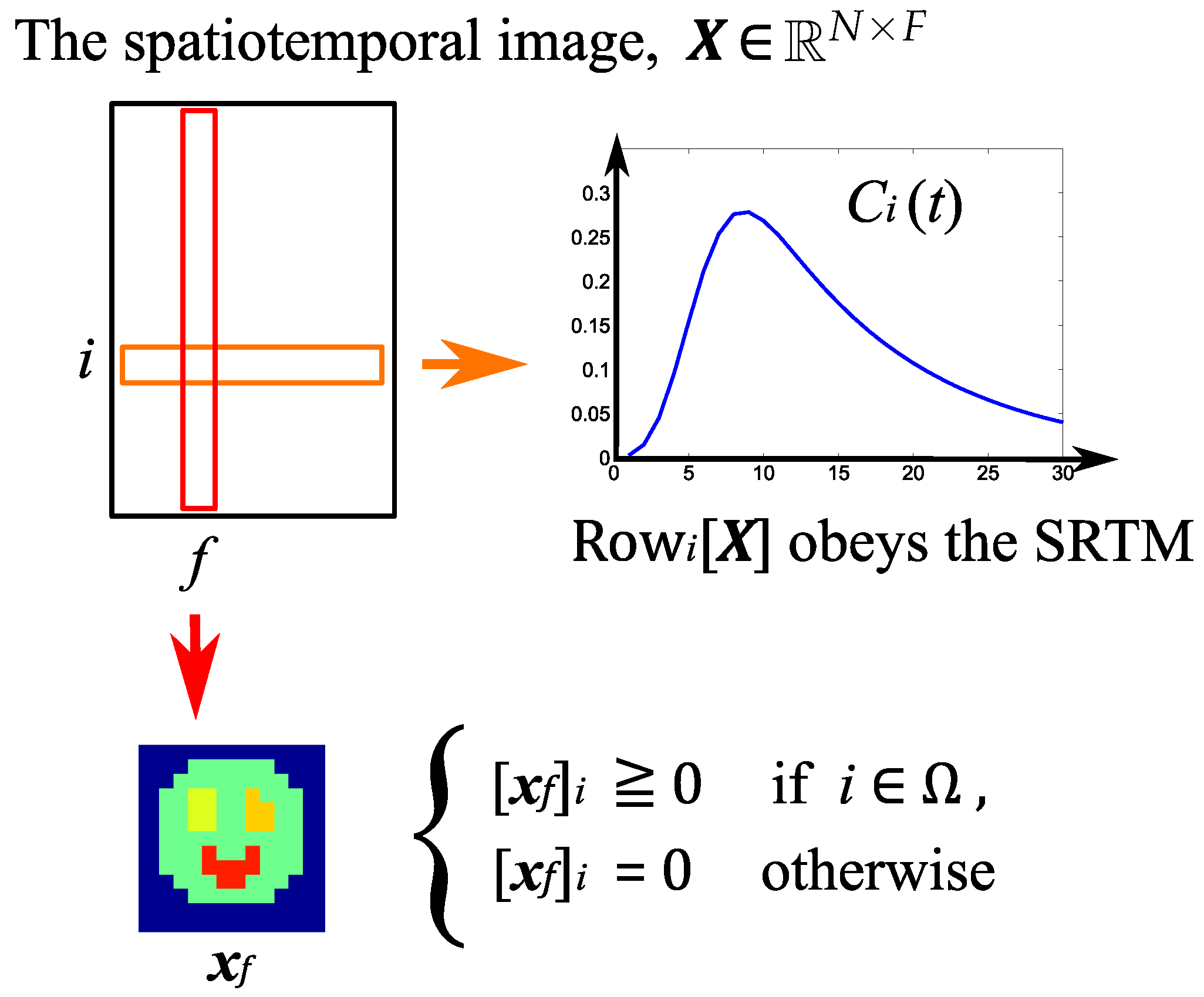
  • Spatial model:
    The nonnegativity of voxel values is assumed. In addition, it is assumed that the foreground/background regions and the reference region in an image are known in advance. The voxel values in the background are set to zero.
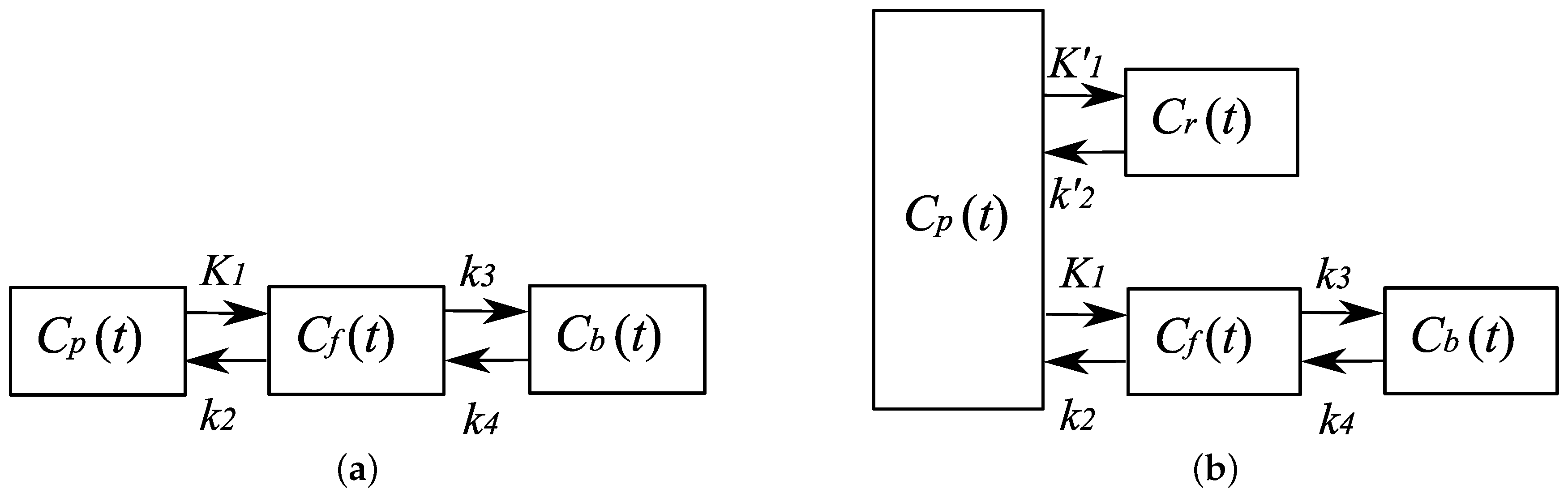
  • Temporal model:
    A compartment model is employed. It is assumed that, given the ligand, one can identify the number of compartments appropriate for the representation of the kinetics. In this paper, we assume a three-compartment model, which is appropriate for a variety of ligands, such as a [ 11 C ]carfentanil and a [ 18 F ]fludeoxyglucose [23,24].
In this article, we clearly define the constrained optimization problem to be solved for the 4D PET image reconstruction and clarify a detailed algorithm that can reach the local minimum of the optimization problem.
In summary, the contributions of this study include:
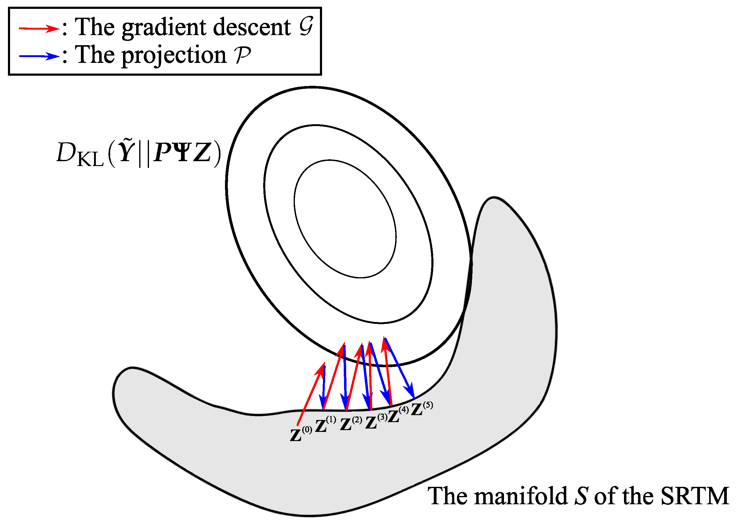
  • A compartment model-based constraint is explicitly introduced in order to constrain the tTACs to the solution space in which the relationships between the tTACs are consistent with the compartment model, while retaining the KL-divergence of data fidelity as a convex function.
  • A constraint of a target region in an image is introduced to restrict the pixel values of the background to be zero.
  • The dependency of the solutions on the initial values is discussed and is experimentally shown.
In the following, first we describe basic materials of mathematics for the PET reconstruction, and then, we describe the compartment model for the PET imaging in Section 2. Next, we describe the proposed method in Section 3. In Section 4, simulation and clinical experimental results are presented. Some behaviors or aspects of the proposed method are discussed in Section 5.

2. Basic Materials

2.1. PET Image Reconstruction

In this study, a vector is denoted by a bold small letter a and a matrix is denoted by a bold capital letter A . A scaler is denoted by a nonbold letter a.
Let an N-dimensional vector x f R N ( f = 1 , 2 , , F ) denote the f-th frame of a temporal series of PET images where N denotes the number of voxels and F denotes the number of frames. Let  t 1 < t 2 < < t F denote the times when the sinograms are measured. Let an M-dimensional vector y f R M denote sinogram data measured by an ideal PET machine at the time t = t f where M denotes the number of bins.
The measurement model of the sinogram is mathematically represented by a linear projection of the PET image as follows:
y ¯ f = P x f ,
where the projection matrix is denoted by an M × N matrix, P , and is assumed to be known in advance. The projection by P corresponds to the Radon transform. Let measured sinogram data corresponding to y ¯ f be denoted by y ˜ f , and let the m-th component of y ¯ f and y ˜ f be denoted by y ¯ f , m and y ˜ f , m , respectively. It is assumed that each component of the measured sinogram data obeys a Poisson distribution such that:
P r ( y ˜ f , m | y ¯ f , m ) = y ¯ f , m y ˜ f , m y ˜ f , m ! exp { y ¯ f , m } .
Conventional methods for 3D PET image reconstruction estimate x f from a measured sinogram y ˜ f . Employing the Poisson model (2), one can estimate x f from y ˜ f by minimizing the KL divergence between y ˜ f and Px f as follows:
x ^ f = arg min x f D KL ( y ˜ f | | Px f ) .
There are several methods that reconstruct 3D PET images by minimizing the KL divergence with some regularizers of the PET image, as follows:
x ^ f = arg min x f D KL ( y ˜ f | | Px f ) + λ η ( x f ) ,
where η ( · ) is a function to penalize the undesirable characteristics of images and λ is a weight parameter. For example, several methods in [10,11,12] set η ( · ) as the total variation. The Expectation Maximization (EM) algorithm and the Ordered Subset EM (OSEM) algorithms are commonly employed for the minimization. Later in this article, a method based on the temporal smooth regularizer is introduced and arranged for a comparison. It is described as follows:
X ^ = arg min X D KL ( Y ˜ | | PX ) + λ 2 f = 1 F 1 | | x f + 1 x f | | 2 2 ,
where X = [ x 1 , x 2 , , x F ] R N × F and Y ˜ = [ y ˜ 1 , y ˜ 2 , , y ˜ F ] R M × F . Problem (5) is configured to make the reconstructed image smooth along the temporal change.

2.2. Compartment Model

There are several kinds of compartment models that represent ligand dynamics [1,25,26]. A three-compartment model [25] consists of three compartments that correspond to plasma, free and bound compartments. The plasma compartment corresponds to the arterial plasma. The ligand transports from the plasma into and back from the free compartment, which is represented by the other two compartments. The free compartment corresponds to the intracellular region, in which the ligand does not bond with receptors.
As shown in Figure 1a, the ligand can transmit only between the plasma compartment and the free compartment. The ligand in the free compartment can also be transmitted to the bound compartment, in which the ligand binds to receptors. Let the ligand concentrations at time t in the plasma, free and bound compartments be denoted by C p ( t ) , C f ( t ) and C b ( t ) , respectively. The three-compartment models have four parameters: K 1 , k 2 , k 3 and k 4 . The dynamics of the ligand transmission are represented by a system of differential equations with the four parameters, as follows:
d C b d t = k 3 C f ( t ) k 4 C b ( t ) ,
d C f d t = K 1 C p ( t ) k 2 C b ( t ) k 3 C f ( t ) + k 4 C b ( t ) .
A PET image captured at time t describes the spatial distribution of C b ( t ) + C f ( t ) , which represents the total ligand concentration in the tissue. A PET image cannot distinguish between the ligand in the free compartment and that in the bound compartment. Let C ( t ) denote the tTAC, where  C ( t ) = C b ( t ) + C f ( t ) . Given C p ( t ) , one can represent C ( t ) d t as follows:
d C d t = K 1 C p ( t ) k 2 C ( t ) .
From the above notations, C ( t ) can be represented with the four free parameters as:
C ( t ) = K 1 θ 2 θ 1 { ( k 3 + k 4 θ 1 ) e θ 1 t + ( θ 2 k 3 k 4 ) e θ 2 t } C p ( t ) ,
where ∗ denotes the convolutional operator, and θ 1 , 2 = 1 2 { k 2 + k 3 + k 4 ± ( k 2 + k 3 + k 4 ) 2 4 k 2 k 4 } . The above equation is widely used for estimating the values of the kinetic parameters in the brain. For example, in [25,27], the model was fit to clearly analyze the transfer of ligands in the ROI (Region Of Interest) where tTACs suffer from severe noise. However, a significant weak point is that one needs to measure not only the tTACs C ( t ) , but also the plasma Time Activity Curves (pTACS) C p ( t ) . The measurement of the pTACs requires the invasive treatment of patients: it requires that patient plasma is sampled for a long time. This is why a Simplified Reference Tissue Model (SRTM) is also clinically used. It is called a reference region in the tissues where no receptor for the ligand exists. Hence, no ligand is bound in the regions. In the compartment of the reference region, the values of k 3 and k 4 are zero. As shown in Figure 1b, let a tTAC in the reference region be denoted by C r ( t ) . Then, given C r ( t ) , the tTACs observed at the i-th voxel C i ( t ) on the outside of the reference region can be represented as follows [23,26]:
C i ( t ) = R 1 C r ( t ) + k 2 R 1 k 2 1 + B P N D C r ( t ) exp k 2 t 1 + B P N D ,
where R 1 = K 1 K 1 = α and B P N D = k 3 k 4 = β . The tTACs satisfy the compartment model only when Equation (10) is satisfied. When one analyzes a temporal series of PET images using SRTM, one manually labels the reference regions in the measured PET images [28,29]. The proposed method introduces an SRTM shown in Equation (10) for the constraint with tTACs.

3. Proposed Method

3.1. Notation

Let a temporal series of measured sinograms be denoted by an M × F matrix, Y ˜ = [ y ˜ 1 , y ˜ 2 , , y ˜ F ] R M × F , and let the spatiotemporal PET images to be reconstructed be denoted by an N × F matrix, X = [ x 1 , x 2 , , x F ] R N × F . Let Row i [ X ] denote the i-th row of a matrix X . Each row of X describes a tTAC observed at the corresponding voxel such that:
Row i [ X ] = [ C i ( t 1 ) , C i ( t 2 ) , , C i ( t F ) ] .
Let a temporal series of sinograms that corresponds linearly to X be denoted by a M × F matrix, Y ¯ = [ y ¯ 1 , y ¯ 2 , , y ¯ F ] R M × F . Similar to the static case in Equation (1), we have:
Y ¯ = P X .
The measured sinograms Y ˜ are assumed to be derived from the Poisson distribution of which the average is Y ¯ . Given Y ˜ , the proposed method estimates the PET images X by solving a constrained optimization problem described below.

3.2. Description of Proposed Method

First, we assume that the whole brain region and reference region for an SRTM in a PET image are known. Let the whole and reference regions be denoted by Ω and Γ , respectively ( Γ Ω ) .
Let N Ω = | Ω | ( N Ω < N ) , and let the j-th voxel in Ω ( j = 1 , 2 , , N Ω ) be denoted by i j . Let a set of indexes J = { i j | j = 1 , 2 , , N Ω } , represent voxels in Ω . An N × N Ω matrix Ψ is defined as Ψ = [ e i 1 , e i 2 , , e i N Ω ] , where all components of the N-dimensional vector e i are zero, except that the i-th component of e i is one: [ e i ] i = 1 . Then, we can represent an entire PET image x f using a lower-dimensional vector z f as follows:
x f = Ψ z f ,
where z f is an N Ω -dimensional vector. The j-th component of z f is a voxel value of the i j -th voxel in x f : [ x f ] i j = [ z f ] j . Let Z = [ z 1 , z 2 , , z F ] . Then, we have:
Y ¯ = P Ψ Z ,
and we can reconstruct PET images by estimating Z . By representing PET images with Z , one can reduce the dimensions of the image representation and impose that the values in the empty backgrounds of PET images are zero.
Let us assume that the tTAC C r ( t ) , which is observed in the reference region Γ , is known. Then, following Equation (10), a tTAC observed on the outside of Γ is consistent with the compartment model only when C i j ( t ) ( i j J ) can be represented with three parameters α j , β j , γ j , as follows:
C i j ( t | α j , β j , γ j ) = α j C r ( t ) + β j γ j C r ( t ) exp β j ( 1 γ j ) α j t .
Let α = [ α 1 , , α N Ω ] T , β = [ β 1 , , β N Ω ] T , γ = [ γ 1 , , γ N Ω ] T , and let a parametric representation of Z in (14) be denoted by Z ( α , β , γ ) such that:
Row j [ Z ( α , β , γ ) ] = [ C i j ( t 1 | α j , β j , γ j ) , C i j ( t 2 | α j , β j , γ j ) , , C i j ( t F | α j , β j , γ j ) ] ( j = 1 , 2 , , N Ω ) .
Each row of Z ( α , β , γ ) denotes the tTAC that is consistent with the tTAC C r ( t ) observed in the reference region Γ . Then, the problem to be solved here is to estimate the parameter values α j , β j , γ j ( j = 1 , 2 , , N Ω ) that minimize the KL divergence with the measured sinograms:
Z ^ = arg min α , β , γ D KL ( Y ˜ | | P Ψ Z ( α , β , γ ) ) .
It should be noted that the reconstructed series of temporal images denoted by Ψ Z ^ satisfies the following constraints: (1) all voxel values are nonnegative; (2) all voxel values in the backgrounds ( Ω ¯ ) are zero; (3) all tTACs in Ω are consistent with the tTAC in the reference region Γ from the viewpoint of the SRTM; and (4) the distance from the sinogram is minimized. A description of the reconstructed image is shown in Figure 2.
However, it is difficult to solve the problem in (17) directly. The objective function D KL ( Y ˜ | | P Ψ Z ( α , β , γ ) ) has 3 × N Ω parameters: α R N Ω , β R N Ω , and γ R N Ω . The PET images X to be reconstructed have N × F voxels in total, and 3 × N Ω is much smaller than N × F . The objective function, however, is not convex in the 3 × N Ω -dimensional kinetic parameter space. Conventional techniques such as the steepest descent method can fail to obtain the appropriate parameter values.
To solve this problem, the proposed method leverages the fact that the target function D KL ( Y ˜ | | P Ψ Z ) is convex with respect to Z . We reformulate Problem (17) into a constrained optimization problem such that:
Z ^ = arg min Z D KL ( Y ˜ | | P Ψ Z ) , s . t . Z S , Z 0 ,
where:
S = { Z ( α , β , γ | C r ( t ) ) | α j R α , β j R β , γ j R γ } .
C r ( t ) , which is assumed to be given in advance, is a tTAC in the region Γ . The minimization of the objective function D KL ( Y ˜ | | P Ψ Z ) can be transformed as:
arg min Z D KL ( Y ˜ | | P Ψ Z ) = m f Y ˜ m f log Y ˜ m f [ P Ψ Z ] m f Y ˜ m f + [ P Ψ Z ] m f = arg min Z m f Y ˜ m f log [ P Ψ Z ] m f + [ P Ψ Z ] m f .
Here, D KL ( Y ˜ | | P Ψ Z ) is convex with respect to Z R N Ω × F and S is a nonconvex set that can be represented by a 3 × N Ω -dimensional manifold in the N Ω × F -dimensional space of Z . The proposed method solves the problem (18) by means of a projected gradient descent. That is, the constrained optimization problem is decomposed into two subproblems. One is a convex optimization problem, such that:
arg min Z D KL ( Y ˜ | | P Ψ Z ) , s . t . Z 0 ,
and the other is a problem of a projection onto the manifold, which is not a convex, but a tractable optimization problem:
arg min Z | | Z ˘ Z | | F 2 , s . t . Z S ,
where Z ˘ is a current value of Z before the projection. The proposed optimization algorithm consists of two steps, i.e., a gradient step and a projection step, as shown in Figure 3. These two steps are applied in order at each iterative update of Z . Let k ( k = 1 , 2 , ) denote the number of the update iteration, and let Z ( k ) denote the initial value of Z at the k-th iteration. The update rule at the gradient step is derived from the gradient of the subproblem (21) as follows:
Z ˘ ( k ) = G [ Z ( k ) ] = Z ( k ) ϵ ( k ) D K L Z ( k ) ,
where ϵ ( k ) is the step size. The update rule at the projection step solves the problem (22) as follows:
Z ( k + 1 ) = P [ Z ˘ ( k ) ] = arg min Z S | | Z ˘ ( k ) Z | | F 2 ,
In summary, the two update rules are applied to Z to obtain Z ( k + 1 ) as follows:
Z ( k + 1 ) = P G [ Z ( k ) ] .
The details of G and P are explained in Section 3.2.1 and Section 3.2.2.

3.2.1. The Gradient Step, G

The gradient of the objective function in (21) is:
D K L Z = Ψ T P T 1 Ψ T P T ( Y ˜ [ P Ψ Z ] ) ,
where 1 = { 1 } M × F and ⊘ denotes the element-wise division operator. Although the update rule in (23) is a basic form for a gradient descent, it is difficult to set each step size appropriately for D KL ( Y ˜ | | P Ψ Z ) . For Z 0 , we can employ a multiplicative update rule [30] to effectively solve Problem (21). From (26), the multiplicative update rule for Z ( k ) described by G is derived as follows:
G [ Z ( k ) ] = Z ( k ) ( Ψ T P T { Y ˜ [ P Ψ Z ( k ) ] } ) [ Ψ T P T 1 ] ,
where ∘ denotes the Hadamard (element-wise) product. This update rule is analogous to that of EM [31,32].

3.2.2. The Projection Step, P

In order to obtain the projection P in (24), a tTAC C i j ( t | α j , β j , γ j ) , which is consistent with the compartment model as shown in (15), is fitted to Row j [ Z ˘ ( k ) ] . Given a reference signal C r ( t ) , Z ˘ ( k ) can be projected onto the manifold S by solving the following minimization problem for each voxel:
minimize α j , β j , γ j g ( α j , β j , γ j ) = f = 1 F | | z j ( t f ) C i j ( t f | α j , β j , γ j ) | | F 2 ,
where z j ( t f ) = Row j [ Z ˘ ( k ) ] ( t f ) . It should be noted that each voxel in Ω has three parameters to be estimated: α j , β j and γ j . Problem (28) can be iteratively solved voxel independently through a gradient descent method as follows:
α j α j ϵ α j g j α j ,
β j β j ϵ β j g j β j ,
γ j γ j ϵ γ j g j γ j ,
where ϵ α j , ϵ β j , ϵ γ j are step sizes. Each derivative is obtained as (32)–(37):
g j α j = f = 1 F 2 { z j ( t f ) α j C r ( t f ) β j γ j h j ( t f | α j , β j , γ j ) } C r ( t f ) β j γ j h j α j ,
h j α j = β j ( 1 γ j ) α j 2 C r ( t ) t exp β j ( 1 γ j ) α j t ,
g j β j = f = 1 F 2 { z j ( t f ) α C r ( t f ) β j γ j h j ( t f | α j , β j , γ j ) } γ j h j ( t f | α j , β j , γ j ) β j γ j h j β j ,
h j β j = ( 1 γ j ) α j C r ( t ) t exp β j ( 1 γ j ) α j t ,
g j γ j = f = 1 F 2 { z j ( t f ) α C r ( t f ) β j γ j h j ( t f | α j , β , j γ j ) } β j h j ( t f | α j , β j , γ j ) β j γ j h j γ j ,
h j γ j = β j α j C r ( t ) t exp β j ( 1 γ j ) α j t ,
where h j ( t | α j , β j , γ j ) = C r ( t ) exp β j ( 1 γ j ) α j t . Let α ^ j , β ^ j , γ ^ j denote the estimated kinetic parameters for the j-th voxel. Then, the projection operator P is given as follows:
P [ Z ˘ ( k ) ] = Z ( α ^ , β ^ , γ ^ ) .
In practice, it should be noted that the gradient descent scheme (29)–(31) can be efficiently computed for all voxels in parallel.  C r ( t ) can be obtained by, for example, averaging temporally-smoothed tTACs in Γ in advance.
In summary, the proposed algorithm is shown in Algorithm 1.
Algorithm 1 Description of proposed method.
  1:
input: An observed temporal series of sinograms Y ˜ , the region Ω where the target object exists and the reference region Γ .
  2:
Ψ is configured based on Ω .
  3:
Initialize X ;
  4:
Initialize Z = Ψ T X ;
  5:
repeat
  6:
 Update Z based on Equation (38);
  7:
 Update Z based on Equation (27);
  8:
 Solve the Problem (28) via the steepest descent method based on gradients (32)–(37);
  9:
until Z converges.
10:
output: X = Ψ Z .

4. Experimental Results

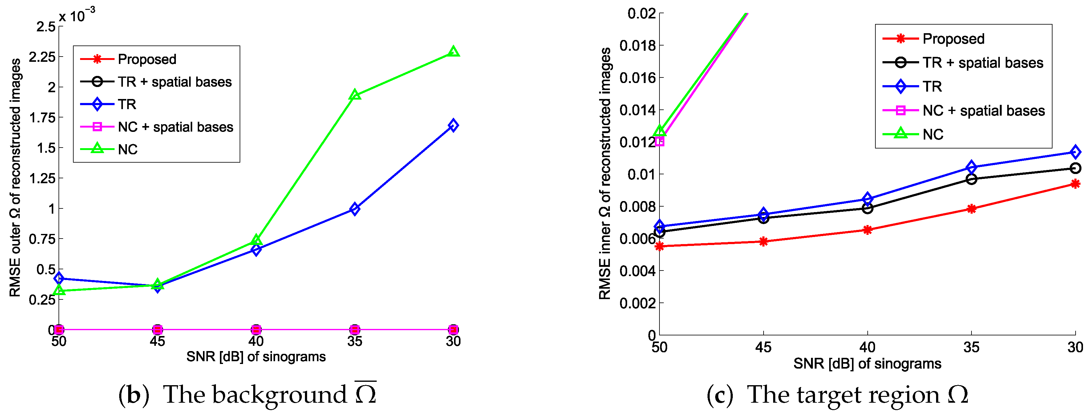
4.1. Evaluation with Simulated Data

We constructed a temporal series of 2D PET images to evaluate the performance of the proposed method. The simulated image X org is first designed to obey the SRTM. The image consists of four regions where the kinetic parameters α , β , γ are different from each other. Given α , β and γ , we generated a tTAC for each pixel in each region respectively based on (15). In order to simulate sinograms with variational Poisson noise levels, we conducted the following procedure: The sinogram data were first obtained from the simulated image as follows:
Y ¯ sml = μ P X org ,
where μ > 0 is a weight parameter that affects the total counts of the sinograms. An artificial measurement of the sinogram, Y ˜ sml , was derived from the Poisson distribution shown in Equation (2). The noise level of Y ˜ sml can be controlled by changing the value of μ .
Multiple reconstruction methods were applied to restore the original image from the simulated measured sinograms Y ˜ sml . The performance was evaluated based on the Normalized Root Mean Squared Error (NRMSE) between the simulated original image X org and the reconstructed one. A comparison evaluation was performed with the methods of which constraints are different from each other. The comparison methods are summarized in Table 1. In Table 1, the method NC (Non-Constraint) minimizes the KL-divergence D KL ( Y ˜ | | PX ) without any constraints nor regularizers [32]. TR (Temporal Regularization) minimizes the KL-divergence with a regularizer that imposes temporal smoothness [22]. The option “+ spatial bases” denotes that spatial image patterns are represented by Ψ Z as shown in (13) in each corresponding method in order to constrain the pixel values outside of the target to be zero. The proposed method minimizes the KL-divergence with respect to the constraint of the manifold and the optimization using the spatial bases. The solver to optimize Problem (5) (TR) is summarized in the Appendix A. The parameter λ in Problem (5), which corresponds to TR in Table 1, was manually tuned with regard to the NRMSE performance that is best for each noise level. The variable Z of the proposed method is initialized with the resultant image of TR + spatial bases. The tTAC in the reference region C r ( t ) was estimated by averaging tTACs in Γ as:
[ C r ( t 1 ) , C r ( t 2 ) , , C r ( t F ) ] = 1 | Γ | i j Γ Row i j [ X ] ,
from the result of TR + spatial bases.
Figure 4a shows the NRMSEs for various Poisson noise levels. Figure 4b shows the Root Mean Squared Errors (RMSEs) calculated only in the backgrounds, and Figure 4c shows the RMSEs calculated only in the target region, Ω . Figure 5 and Figure 6 show the reconstructed images and tTACs where the SNR of the measured sinograms is 50 dB (Figure 5) and 35 dB (Figure 6). All the simulational resultant images can be seen in the Supplementary Material S1. The SNR of the measured sinograms Y ˜ sml is derived from the error between Y ˜ sml and Y ¯ sml . The NRMSE of NC deviates with a high noise level in Figure 4. The performance was drastically improved using the temporal regularizer. The performance was also improved especially with a high noise level when the spatial bases is introduced to TR. Furthermore, the proposed method, which uses constraints of the SRTM and spatial bases, outperformed the other methods. Not only RMSEs in the backgrounds, but also RMSEs in the target region were reduced in Figure 4b,c when the spatial bases are used. The usefulness of the spatial bases and the model constraint was confirmed.
Furthermore, Figure 7 shows the behavior of the convergence of the proposed method with respect to the number of the projection obtained from different initial values. For the comparison purpose, we employed four different reconstruction methods, TR, TR + spatial bases, NC, and NC + spatial bases, shown in Table 1, all of which reconstruct PET images via convex optimization. Each panel shows four graphs obtained from identical sinogram data with different initialization, and the graphs shown in different panels are obtained from different SN ratios of the sinogram. Since the proposed method solves a nonconvex optimization problem, the performance of the proposed method depends on the initial value of Z . It can be said the spatial bases are also effective for achieving the better initialization of the proposed method.

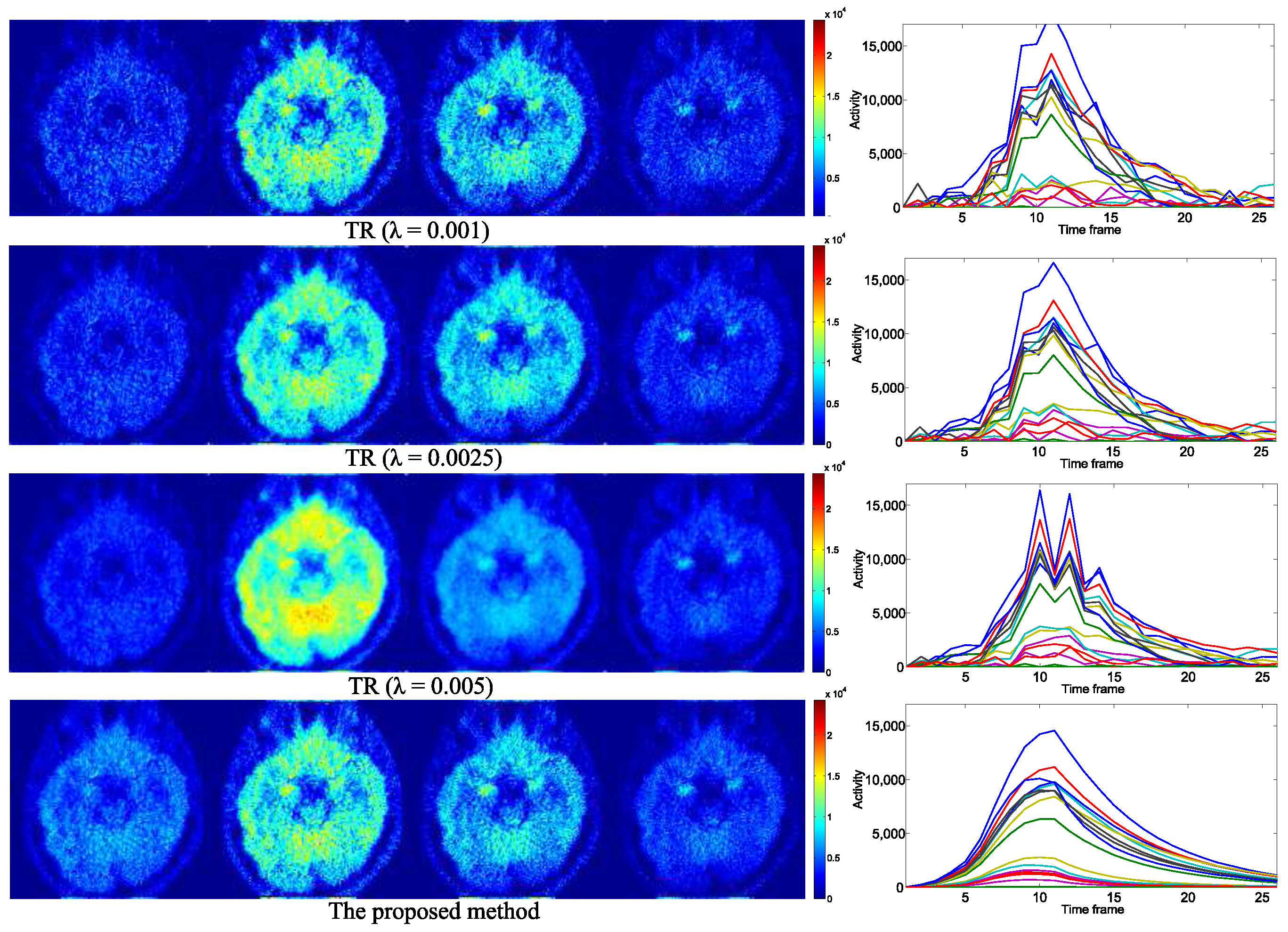
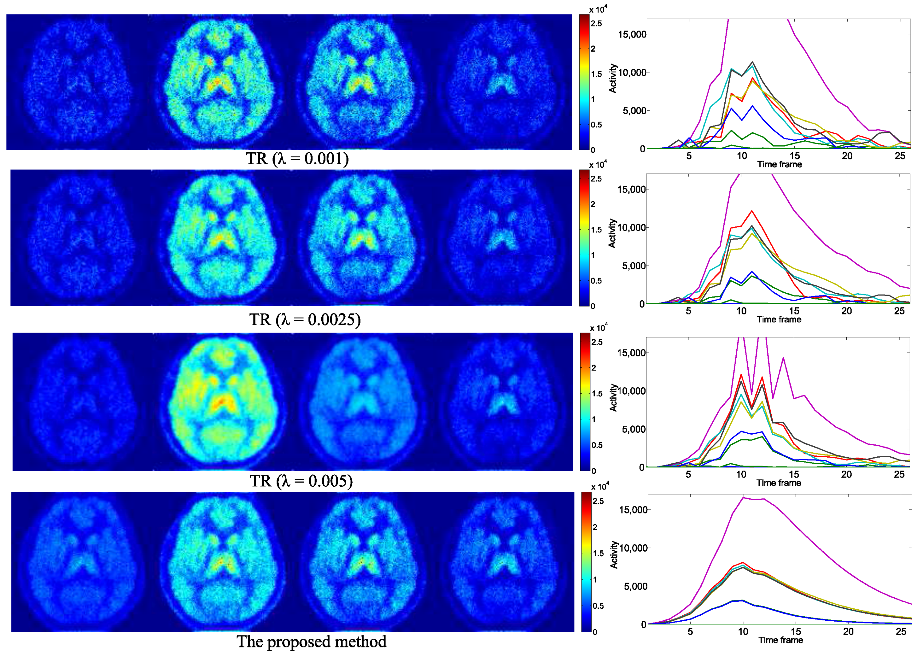
4.2. Practical PET Images Reconstruction from Clinical Sinograms

We also applied the proposed method to clinical data. Sinogram data were obtained by injecting [ 11 C ]carfentanil into a patient. The size of the resultant 3D PET image is 96 × 96 × 63 ( M = 580 , 608 ) , and the number of time frames is F = 26 . The reference region Γ and the target region Ω were manually obtained from the resultant image of OSEM [2,28,29]. The tTAC in the reference region C r ( t ) was estimated by averaging tTACs in Γ as (40). The initial value for the proposed method is given from the result of TR with λ = 0.0025 .
Figure 8, Figure 9 and Figure 10 show the reconstructed images of TR with variational parameters ( λ = 0.005 , 0.0025 , 0.001 ) and the proposed method. The differences between the proposed method and the others are especially clear in the first and fourth time frames. Although the resultant images of TR vary sensitively with changes in λ , the images reconstructed by the proposed method are both distinct and smooth compared to the other images.
We employed the Coefficient of Variation (CV) [33] for the validation of the results obtained from clinical data. The CV value is defined as (41) and is evaluated for each ROI (Region Of Interest) that is manually labeled by an expert. In each ROI, the kinetic parameters are known to be identical, and hence, tTACs are ideally the same at every location.
CV ¯ ( X ξ ) = 1 F f = 1 F CV ( X ξ , f ) = 1 F f = 1 F σ ( X ξ , f ) μ ( X ξ , f ) ,
where X ξ , f denotes a set of voxel values observed in the ξ -th ROI at the f-th frame and ξ and f denote the indices of the ROI and the frame, respectively. σ ( X ξ , f ) and μ ( X ξ , f ) denote the standard deviation and the mean of X ξ , f , respectively. CV ¯ ( X ξ ) should be small if 4D PET images are accurately reconstructed. The evaluated values are shown in Table 2. The ROIs for which we evaluated CV values are as follows: cerebellum ( ξ = 1 ), occipital lobe ( # 2 ), frontal lobe ( # 3 ), temporal lobe ( # 4 ), thalamus ( # 5 ), putamen ( # 6 ) and caudate nucleus ( # 7 ), respectively. The parameter λ for TR was manually tuned to achieve the best results. The proposed method was initialized from the results obtained by TR with λ = 0.0025 . For all ROIs, the proposed method outperformed TR: the images reconstructed by the proposed method have more uniform voxel values in each ROI in each time.

5. Discussion

5.1. Optimization Strategy

In this study, we considered solving the minimization problem of the KL-divergence between measured sinograms and simulated sinograms, which are modeled with kinetic parameters as shown in (17). In addition, we incorporated a boundary prior of a brain region by using nonnegative spatial bases. Note that our objective is different from conventional penalized/regularized methods such as temporal or spatial smoothing because the compartment model strictly satisfies the theoretical consistency of 4D PET images. Furthermore, we do not need to tune any trade-off parameters unlike penalized methods. The problem here is that the cost function in (17) is nonconvex with respect to kinetic parameters, and it is very difficult to solve directly.
In order to solve the nonconvex optimization problem (17), we have rewritten (17) as (18), which consists of the convex objective function and the nonconvex constraint set. Note that the problems (17) and (18) are theoretically equivalent; however, the parameter space is expanded from 3 × N Ω to N Ω × F . This modification relaxed the nonconvex objective function to the convex objective function which helps to apply the projected gradient method for our problem. The proposed optimization algorithm consists of two steps: the gradient step to minimize the objective function and the projection step to put the 4D PET images on the manifold based on the SRTM.
The proposed algorithm of the projected gradient scheme is similar to those of [15,31,34] as also described in Section 5.3, but is a more generalized one. The gradient step of the proposed algorithm is based on a gradient descent that substantially includes the EM update used in [15,34]. Furthermore, the estimation of the kinetic parameters is solved in the proposed method via a gradient descent scheme where each derivative is explicitly used. The conventional methods solve the estimation of the kinetic parameters through numerical analytic approaches where derivatives are implicit and approximated.

5.2. Sensitivity to Initialization

As the optimization problem to be solved is nonconvex, the reconstruction results depend on the initial value of the coefficient, Z . From Figure 7, it can be said that the better the initialization adopted, the better the performance of the proposed method because of the nonconvexity of the manifold. Thus, the proposed method using the SRTM would always outperform the other regularization-based methods where the SRTM is not used as a constraint. As shown in Figure 7, the TR-based initialization always reconstructed images that have better NRMSE than the NC-based ones. NC-based methods reconstruct images with less constraints/regularization than TR-based ones, and hence, the images reconstructed by the NC-based methods are more consistent with the measured sinograms that are contaminated by Poisson noises: PET images reconstructed by NC-based methods would more easily overfit to the noisy data, and the NRMSE of these images rapidly increased with respect to the Poisson noise level of the sinogram data, as shown in Figure 7. The initialization via NC-based methods would be useful when one prefers PET images that are more consistent with measured data (often contaminated with noise), and the initialization with TR-based methods is recommended if images with less NRMSE should be reconstructed. One can of course introduce the knowledge of the target region for the initialization in order to improve NRMSE.

5.3. Related Works

There exist many methods for 4D PET image reconstruction, and our proposed method has strong relationships especially with the methods that constrain tTACs based on the compartment model [5,14,31,35,36]. First of all, we have to point out that none of these papers explicitly show a constrained optimization problem to be solved, but show only corresponding sub-problems. This fact makes it difficult to discuss the problem of 4D PET image reconstruction and its corresponding solution algorithm. As far as we know, none of the existing compartment model-based methods for the 4D PET image reconstruction except one method [34] proposed by Gravel and Reader (GR) directly use the nonlinear model derived from the compartment model, but use some linearly approximated models for the constraint, as described in their paper [34]. Only the GR method explicitly introduces the nonlinear kinetic model derived from the compartment model to constrain the solution space. The paper [34], though, does not explicitly show the main optimization problem to be solved, and no details of the solution algorithm for satisfying the nonlinear constraint are described. In addition, the sensitivity of the results to the initial values is not discussed. We, on the other hand, clearly show the problem to be solved as in (18), discussing the sensitivity to the initialization and experimentally demonstrating the results about the sensitivity. Furthermore, the convergence of the GR method would not be guaranteed. The GR method updates the reference signal C r ( t ) every other iteration. This would lead to the manifold spanned by the SRTM being reshaped every other iteration, and projections could sometimes diverge. On the other hand, C r ( t ) is fixed in the proposed method, which is given from the temporally-smoothed image by TR in this paper. The fixed shape of the manifold would ensure the convergence of the proposed method. The constraint about the target/background regions in images is also newly incorporated in the problem of the compartment-model-based 4D PET image reconstruction.

6. Conclusions

In this study, we proposed a parametric PET image reconstruction technique. A set of nonnegative spatial bases is introduced to ignore noise in backgrounds and explicitly describe the image region. Iterative projections to an SRTM are introduced to parametrically reconstruct a PET image. The advantages of using the spatial bases and the SRTM are examined by comparing them with conventional regularized methods. The experimental results showed that the proposed method outperforms the conventional regularized methods under the existence of severe noise in observed sinograms.

Supplementary Materials

The following are available online at www.mdpi.com/1099-4300/19/11/629/s1, The supplementary material S1 include all the resultant images of the simulational experiments in Section 4.1.

Acknowledgments

This study was supported by JSPS KAKENHI Grant Numbers 26108003 and 15K16067.

Author Contributions

Tatsuya Yokota and Hidekata Hontani conceived of the paper. Naoki Kawamura and Tatsuya Yokota designed the algorithms and performed the experiments. Naoki Kawamura, Tatsuya Yokota and Hidekata Hontani discussed the methodology and wrote the paper. Muneyuki Sakata and Yuichi Kimura provided the clinical data, some useful comments and some revisions of the paper. All authors have read and approved the final manuscript.

Conflicts of Interest

The authors declare no conflict of interest.

Appendix A

In this Appendix, we explain an optimization algorithm to solve Problem (5) using a set of spatial bases Ψ . Problem (5) can be transformed as:
Z ^ = arg min Z F ( Z ) = D KL ( Y ˜ | | P Ψ Z ) + λ 2 | | Ψ Z L | | F 2 ,
where L is a given matrix to differentiate matrix Ψ Z along columns. The derivative of Problem (A1) is:
F Z = Ψ T P T 1 Ψ T P T ( Y ˜ [ P Ψ Z ] ) + λ Ψ T Ψ Z L L T .
Then, the multiplicative update rule to solve Problem (A1) is given by:
Z ( k + 1 ) Z ( k ) ( Ψ T P T { Y ˜ [ P Ψ Z ( k ) ] } + [ λ Ψ T Ψ Z ( k ) L L T ] ) ( Ψ T P T 1 + [ λ Ψ T Ψ Z ( k ) L L T ] + ) ,
where [ · ] and [ · ] + are projection operators, such that [ A ] v w = | min ( A v w , 0 ) | and [ A ] + v w = max ( A v w , 0 ) for an arbitrary matrix A .

References

  1. Watabe, H.; Ikoma, Y.; Kimura, Y.; Naganawa, M.; Shidahara, M. PET kinetic analysis—Compartmental model. Ann. Nucl. Med. 2006, 20, 583–588. [Google Scholar] [CrossRef] [PubMed]
  2. Hudson, H.M.; Larkin, R.S. Accelerated image reconstruction using ordered subsets of projection data. IEEE Trans. Med. Imaging 1994, 13, 601–609. [Google Scholar] [CrossRef] [PubMed]
  3. Fessler, J.A.; Rogers, W.L. Spatial resolution properties of penalized-likelihood image reconstruction: Space-invariant tomographs. IEEE Trans. Image Process. 1996, 5, 1346–1358. [Google Scholar] [CrossRef] [PubMed]
  4. Qi, J.; Leahy, R.M.; Cherry, S.R.; Chatziioannou, A.; Farquhar, T.H. High-resolution 3D Bayesian image reconstruction using the microPET small-animal scanner. Phys. Med. Biol. 1998, 43, 1001–1013. [Google Scholar] [CrossRef] [PubMed]
  5. Wang, G.; Qi, J. Generalized algorithms for direct reconstruction of parametric images from dynamic PET data. IEEE Trans. Med. Imaging 2009, 28, 1717–1726. [Google Scholar] [CrossRef] [PubMed]
  6. Ross, S.Q. Clear WhitePaper; GE Healthcare: Little Chalfont, UK, 2014; pp. 1–9. [Google Scholar]
  7. Mumcuoglu, E.U.; Leahy, R.; Cherry, S.R.; Zhou, Z. Fast gradient-based methods for Bayesian reconstruction of transmission and emission PET images. IEEE Trans. Med. Imaging 1994, 13, 687–701. [Google Scholar] [CrossRef] [PubMed]
  8. Lee, J.S.; Lee, D.D.; Choi, S.; Park, K.S.; Lee, D.S. Non-negative matrix factorization of dynamic images in nuclear medicine. In Proceedings of the IEEE Nuclear Science Symposium Conference Record, San Diego, CA, USA, 4–10 November 2001; Volume 4, pp. 2027–2030. [Google Scholar]
  9. Lee, J.S.; Lee, D.D.; Choi, S.; Lee, D.S. Application of nonnegative matrix factorization to dynamic positron emission tomography. In Proceedings of the 3rd International Conference on Independent Component Analysis and Blind Signal Separation, San Diego, CA, USA, 9–13 December 2001; pp. 629–632. [Google Scholar]
  10. Pustelnik, N.; Chaux, C.; Pesquet, J.C.; Comtat, C. Parallel algorithm and hybrid regularization for dynamic PET reconstruction. In Proceedings of the IEEE Nuclear Science Symposium Conference Record, Knoxville, TN, USA, 30 October–6 November 2010; pp. 2423–2427. [Google Scholar]
  11. Ahn, S.; Kim, S.M.; Son, J.; Lee, D.S.; Sung Lee, J. Gap compensation during PET image reconstruction by constrained, total variation minimization. Med. Phys. 2012, 39, 589–602. [Google Scholar] [CrossRef] [PubMed]
  12. Burger, M.; Müller, J.; Papoutsellis, E.; Schönlieb, C.B. Total variation regularization in measurement and image space for PET reconstruction. Inverse Probl. 2014, 30, 105003. [Google Scholar] [CrossRef]
  13. Li, T.; Thorndyke, B.; Schreibmann, E.; Yang, Y.; Xing, L. Model-based image reconstruction for four-dimensional PET. Med. Phys. 2006, 33, 1288–1298. [Google Scholar] [CrossRef] [PubMed]
  14. Kamasak, M.E.; Bouman, C.A.; Morris, E.D.; Sauer, K. Direct reconstruction of kinetic parameter images from dynamic PET data. IEEE Trans. Med. Imaging 2005, 24, 636–650. [Google Scholar] [CrossRef] [PubMed]
  15. Matthews, J.C.; Angelis, G.I.; Kotasidis, F.A.; Markiewicz, P.J.; Reader, A.J. Direct reconstruction of parametric images using any spatiotemporal 4D image based model and maximum likelihood expectation maximisation. In Proceedings of the Nuclear Science Symposium Conference Record, Knoxville, TN, USA, 30 October–6 November 2010; pp. 2435–2441. [Google Scholar]
  16. Reader, A.J.; Zaidi, H. Advances in PET image reconstruction. PET Clin. 2007, 2, 173–190. [Google Scholar] [CrossRef] [PubMed]
  17. Vardi, Y.; Shepp, L.; Kaufman, L. A statistical model for positron emission tomography. J. Am. Stat. Assoc. 1985, 80, 8–20. [Google Scholar] [CrossRef]
  18. Carson, R.E.; Yan, Y.; Daube-Witherspoon, M.E.; Freedman, N.; Bacharach, S.L.; Herscovitch, P. An approximation formula for the variance of PET region-of-interest values. IEEE Trans. Med. Imaging 1993, 12, 240–250. [Google Scholar] [CrossRef] [PubMed]
  19. Barrett, H.H.; Wilson, D.W.; Tsui, B.M. Noise properties of the EM algorithm. I. Theory. Phys. Med. Biol. 1994, 39, 833. [Google Scholar] [CrossRef] [PubMed]
  20. Fessler, J.A. Penalized weighted least-squares image reconstruction for positron emission tomography. IEEE Trans. Med. Imaging 1994, 13, 290–300. [Google Scholar] [CrossRef] [PubMed]
  21. Gerchberg, R. Super-resolution through error energy reduction. J. Mod. Opt. 1974, 21, 709–720. [Google Scholar] [CrossRef]
  22. Wernick, M.N.; Infusino, E.J.; Milosevic, M. Fast spatio-temporal image reconstruction for dynamic PET. IEEE Trans. Med. Imaging 1999, 18, 185–195. [Google Scholar] [CrossRef] [PubMed]
  23. Gunn, R.N.; Lammertsma, A.A.; Hume, S.P.; Cunningham, V.J. Parametric imaging of ligand-receptor binding in PET using a simplified reference region model. Neuroimage 1997, 6, 279–287. [Google Scholar] [CrossRef] [PubMed]
  24. Turkheimer, F.E.; Edison, P.; Pavese, N.; Roncaroli, F.; Anderson, A.N.; Hammers, A.; Gerhard, A.; Hinz, R.; Tai, Y.F.; Brooks, D.J. Reference and target region modeling of [11C]-(R)-PK11195 brain studies. J. Nucl. Med. 2007, 48, 158–167. [Google Scholar] [PubMed]
  25. Logan, J.; Fowler, J.S.; Volkow, N.D.; Wolf, A.P.; Dewey, S.L.; Schlyer, D.J.; MacGregor, R.R.; Hitzemann, R.; Bendriem, B.; Gatley, S.J.; et al. Graphical analysis of reversible radioligand binding from time—Activity measurements applied to [N-11C-methyl]-(-)-cocaine PET studies in human subjects. J. Cereb. Blood Flow Metab. 1990, 10, 740–747. [Google Scholar] [CrossRef] [PubMed]
  26. Lammertsma, A.A.; Hume, S.P. Simplified reference tissue model for PET receptor studies. Neuroimage 1996, 4, 153–158. [Google Scholar] [CrossRef] [PubMed]
  27. Logan, J. Graphical analysis of PET data applied to reversible and irreversible tracers. Nucl. Med. Biol. 2000, 27, 661–670. [Google Scholar] [CrossRef]
  28. Yaqub, M.; Van Berckel, B.N.; Schuitemaker, A.; Hinz, R.; Turkheimer, F.E.; Tomasi, G.; Lammertsma, A.A.; Boellaard, R. Optimization of supervised cluster analysis for extracting reference tissue input curves in (R)-[11C] PK11195 brain PET studies. J. Cereb. Blood Flow Metab. 2012, 32, 1600–1608. [Google Scholar] [CrossRef] [PubMed] [Green Version]
  29. Wu, Y.; Carson, R.E. Noise reduction in the simplified reference tissue model for neuroreceptor functional imaging. J. Cereb. Blood Flow Metab. 2002, 22, 1440–1452. [Google Scholar] [CrossRef] [PubMed]
  30. Lee, D.D.; Seung, H.S. Algorithms for non-negative matrix factorization. In Advances in Neural Information Processing Systems 13 (NIPS 2000); Leen, T.K., Dietterich, T.G., Tresp, V., Eds.; MIT Press: Cambridge, MA, USA, 2001. [Google Scholar]
  31. Reader, A.J.; Matthews, J.C.; Sureau, F.C.; Comtat, C.; Trebossen, R.; Buvat, I. Iterative kinetic parameter estimation within fully 4D PET image reconstruction. In Proceedings of the IEEE Nuclear Science Symposium Conference Record, San Diego, CA, USA, 29 October–1 November 2006; Volume 3, pp. 1752–1756. [Google Scholar]
  32. Shepp, L.A.; Vardi, Y. Maximum likelihood reconstruction for emission tomography. IEEE Trans. Med. Imaging 1982, 1, 113–122. [Google Scholar] [CrossRef] [PubMed]
  33. Logan, J.; Fowler, J.S.; Volkow, N.D.; Wang, G.J.; Ding, Y.S.; Alexoff, D.L. Distribution volume ratios without blood sampling from graphical analysis of PET data. J. Cereb. Blood Flow Metab. 1996, 16, 834–840. [Google Scholar] [CrossRef] [PubMed]
  34. Gravel, P.; Reader, A.J. Direct 4D PET MLEM reconstruction of parametric images using the simplified reference tissue model with the basis function method for [11C] raclopride. Phys. Med. Biol. 2015, 60, 4533–4549. [Google Scholar] [CrossRef] [PubMed]
  35. Wang, G.; Qi, J. Direct estimation of kinetic parametric images for dynamic PET. Theranostics 2013, 3, 802–815. [Google Scholar] [CrossRef] [PubMed]
  36. Tsoumpas, C.; Turkheimer, F.E.; Thielemans, K. A survey of approaches for direct parametric image reconstruction in emission tomography. Med. Phys. 2008, 35, 3963–3971. [Google Scholar] [CrossRef] [PubMed]
Figure 1. (a) Three-compartment model. (b) Simplified Reference Tissue Model (SRTM).
Entropy 19 00629 g001
Figure 2. Description of reconstructed image through the proposed method.
Entropy 19 00629 g002
Figure 3. Illustration of the proposed algorithm. Red arrows indicate multiplicative update operations G , and blue arrows indicate projections onto sets spanned by the SRTM P .
Entropy 19 00629 g003
Figure 4. NRMSE and RMSE results in terms of Poisson noise level. Each graph (ac) is different in regions where the error is evaluated: (a) NRSME in whole images, (b) RMSE only in backgrounds and (c) RMSE only in the target region, Ω .
Entropy 19 00629 g004aEntropy 19 00629 g004b
Figure 5. Illustrations of three time frames picked from reconstructed image (top) and some corresponding tTACs (bottom) for each method. The SNR of simulated sinograms is 50 dB.
Entropy 19 00629 g005
Figure 6. Illustrations of three time frames picked from reconstructed image (top) and some corresponding tTACs (bottom) for each method. SNR of simulated sinograms is 35 dB.
Entropy 19 00629 g006
Figure 7. NRMSE improvement of proposed method in terms of the number of projections, k. The colors of curves vary in initialization methods, which give initial values of Z to the proposed method. The noise level of Y ˜ sml varies in each graph: (a) 45 dB, (b) 40 dB, (c) 35 dB and (d) 30 dB.
Entropy 19 00629 g007aEntropy 19 00629 g007b
Figure 8. PET Data #1: Illustrations of reconstructed image with multiple methods (left) and some of their corresponding tissue Time Activity Curves (tTACs) (right). From left to right, four of 26 time frames (7, 10, 13 and 16) are described for each method (left).
Entropy 19 00629 g008
Figure 9. PET Data #2: Illustrations of reconstructed image with multiple methods (left) and some of their corresponding tTACs (right). From left to right, four of 26 time frames (7, 10, 13 and 16) are described for each method (left).
Entropy 19 00629 g009
Figure 10. PET Data #3: Illustrations of reconstructed image with multiple methods (left) and some of their corresponding tTACs (right). From left to right, four of 26 time frames (7, 10, 13 and 16) are described for each method (left).
Entropy 19 00629 g010
Table 1. Correspondence of notations of methods and their constraints for comparison. NC, Non-Constraint; TR, Temporal Regularization.
Notations of MethodsProblems to Be Optimized
NC min X D KL ( Y ˜ | | PX ) .
NC + spatial bases min Z D KL ( Y ˜ | | P Ψ Z ) .
TR min X D KL ( Y ˜ | | PX ) + λ 2 f = 1 F 1 | | x f + 1 x f | | 2 2 .
TR + spatial bases min Z D KL ( Y ˜ | | P Ψ Z ) + λ 2 f = 1 F 1 | | Ψ ( z f + 1 z f ) | | 2 2 .
Proposed min Z D KL ( Y ˜ | | P Ψ Z ) , s . t .   Z S ,   Z 0 .
Table 2. CV ¯ ( X ξ ) calculated in each ROI w.r.t. variational methods.
DataMethodsROI #1ROI #2ROI #3ROI #4ROI #5ROI #6ROI #7
PET Data # 1 TR ( λ = 0.005 )0.5070.6630.5150.6450.6600.4860.647
Proposed0.1740.3020.2190.2360.2140.2400.304
PET Data # 2 TR ( λ = 0.0025 )0.8591.010.8640.7951.1660.7450.752
Proposed0.1360.2450.1640.1240.1340.1650.153
PET Data # 3 TR ( λ = 0.005 )0.7100.8120.6400.6160.6180.6160.772
Proposed0.2400.2950.2510.1990.2400.2210.351

