Article

Two-Party Zero-Error Function Computation with Asymmetric Priors †

1
The Pennsylvania State University, University Park, PA 16802, USA
2
Raytheon BBN Technologies, Cambridge, MA 02138, USA
3
Army Research Laboratory, Adelphi, MD 20783, USA
*
Author to whom correspondence should be addressed.
Earlier versions of this work have partially appeared at the IEEE GlobalSIP Symposium on Network Theory, December 2013, IEEE Data Compression Conference (DCC’14), March 2014, and IEEE Data Compression Conference (DCC’16), March 2016.
Entropy 2017, 19(12), 635; https://doi.org/10.3390/e19120635
Submission received: 11 July 2017 / Revised: 25 October 2017 / Accepted: 13 November 2017 / Published: 23 November 2017
(This article belongs to the Special Issue Network Information Theory)

Abstract

:
We consider a two party network where each party wishes to compute a function of two correlated sources. Each source is observed by one of the parties. The true joint distribution of the sources is known to one party. The other party, on the other hand, assumes a distribution for which the set of source pairs that have a positive probability is only a subset of those that may appear in the true distribution. In that sense, this party has only partial information about the true distribution from which the sources are generated. We study the impact of this asymmetry on the worst-case message length for zero-error function computation, by identifying the conditions under which reconciling the missing information prior to communication is better than not reconciling it but instead using an interactive protocol that ensures zero-error communication without reconciliation. Accordingly, we provide upper and lower bounds on the minimum worst-case message length for the communication strategies with and without reconciliation. Through specializing the proposed model to certain distribution classes, we show that partially reconciling the true distribution by allowing a certain degree of ambiguity can perform better than the strategies with perfect reconciliation as well as strategies that do not start with an explicit reconciliation step. As such, our results demonstrate a tradeoff between the reconciliation and communication rates, and that the worst-case message length is a result of the interplay between the two factors.

1. Introduction

Consider a scenario in which two parties make a query over distributed correlated databases. Each party observes data from one database, whereas the query has to be evaluated over the data observed by both users separately. Suppose that one party knows all data combinations that may lead to an answer to some query, whereas the other party is missing some of these combinations. The parties are allowed to communicate with each other. The goal is to find the minimum amount of communication required so that both parties can retrieve the correct answer for any query. We model this scenario as interactive communication in which two parties interact to compute a function of two correlated discrete memoryless sources. Each source is observed by one party. One party knows the true joint distribution of the sources, whereas the other party is missing some source pairs that may occur with positive probability and assumes another distribution in which these missing pairs have zero probability. Communication takes place in multiple interactive rounds, at the end of which a function of the two correlated sources has to be computed at both parties with zero-error. We study the impact of this partial knowledge about the true distribution on the worst-case message length.
In a function computation scenario, one party observes a random variable X, whereas the other party observes a random variable Y, where each realization of ( X , Y ) is generated from some probability distribution p X Y . The two parties wish to compute a function f ( X , Y ) by exchanging a number of messages in multiple rounds. Conventionally, the true distribution from which the sources are generated is available as common knowledge to both parties. This work extends this framework to the scenario in which the true distribution of the sources is available at one of the communicating parties only, while the distribution assumed at the other party has missing information compared to the true distribution. That is, the second party has only partial knowledge about the source pairs that are realized with positive probability according to the true distribution.
In order to identify the impact of partial information on the worst-case message length, we consider three interactive communication protocols. The first interactive protocol we consider is to reconcile the partial information between the two parties in a way to allow the second party to learn the true joint distribution, and then utilize the true distribution for function computation. The reconciliation stage transforms the problem into the conventional zero-error function computation problem with zero-error. Although this is a natural approach in that it ensures that both sides are in agreement about the true distribution, this protocol requires additional bits to be transmitted between the two parties for reconciling the distribution information, which, in turn may increase the overall message length. The second protocol we consider provides an alternative interaction strategy in which the two parties do not reconcile the true distribution, but instead use a function computation strategy that allows error-free computation under the distribution uncertainty. In doing so, this protocol alleviates the costs that may have incurred for reconciling the distributions. The message length for the function computation part, however, may be larger compared to that of the previous scheme. The last interaction protocol quantifies a trade-off between the two interaction protocols, by allowing the two parties to partially reconcile the distributions. In this protocol, each party learns the true distribution up to a class of distributions. The function computation step then ensures error-free computation under any distribution within the reconciled class of distributions. By doing so, we create different levels of common knowledge about the distribution to investigate the relation between the cost of various degrees of partial reconciliation and the resulting compression performance.
By leveraging the proposed interaction protocols, we identify the conditions under which it is better or worse to reconcile the partial information than to not reconcile the distributions, i.e., using a zero-error encoding scheme with possibly increased message length. Accordingly, we develop upper and lower bounds on the worst-case zero-error message length for computing the function at both parties under different reconciliation and communication strategies. Our results demonstrate that, reconciling the partial information, although often reducing the communication cost, may or may not reduce the overall worst-case message length. In effect, the worst-case message length results from an interplay between reconciliation and communication costs. As such, partial reconciliation of the true distribution is sometimes strictly better than the remaining two interaction strategies.

Related Work

For the setting when both parties know the true joint distribution of the sources, interactive communication strategies have been studied in [1] to enable both sides to learn the source observed by the other party with zero-error. Reference [2] has considered the impact of the number of interaction rounds on the worst-case message length, as well as upper and lower bounds on the worst-case message length. The optimal zero-error communication strategy for minimizing the worst-case message length, even for the setting in which the communicating parties know the exact true distribution of the sources, has since been an open problem. The zero-error communication problem has also been considered for communicating semantic information [3,4]. Our work is also related to the field of communication complexity, which studies the minimum amount of communication required to compute a function of two sources [5]. Known as the direct-sum theorem, it was shown in [6] that computing multiple instances of a function can reduce the minimum amount of communication required per instance. The main distinction between the communication-complexity approaches and the setups from [1,2] is that the models from [1,2] emphasize utilizing the source distribution and in particular its support set to reduce the amount of communication, which is also referred to as the computation of a partial function ([7], Section 4.7).
In addition to the zero-error setup, interactive communication has also been considered for computing a function at one of the communicating parties with vanishing error probability [8]. Subsequently, interactive communication has been considered for computing a function of two sources simultaneously at both parties with vanishing error probability [9]. The two-party scenario has been extended to a multi-terminal function computation setup in [10], in which each party observes an independent source and broadcasts its message to all the nodes in the network. A related study in [11] investigates the role of side information when communicating interactively a source known by one party to another with vanishing error. Interactive communication has also been leveraged in [11] for one-way recovery of a source known by one party at the other side with vanishing error in the presence of side information.
This work is also related to zero-error communication strategies in non-interactive data compression scenarios. In particular, we leverage graphical representations of the confusable source and distribution terms, which are reminiscent of characteristic graphs introduced in [12] to study the zero-error capacity of a channel. Subsequently, characteristic graphs have been utilized for zero-error compression of a source in the presence of decoder side information [13,14]. They have been utilized to characterize graph entropy and chromatic entropy in [15,16], respectively, in [8] to characterize the rate region for the lossless computation of a function, and in [17] to obtain achievable rates for lossy function computation. Such graphical representations have also been leveraged for non-interactive set reconciliation [18]. Another relevant application is zero-error source coding with compound decoder side information considered in [19].
Many existing and emerging network applications, e.g., sensor networks, cyber-physical systems, social media, and semantic networks, facilitate interaction between multiple terminals to share information towards achieving a common objective [20,21,22,23]. As such, it is essential for such systems to mitigate the ambiguities that may result from the imperfect knowledge available at the communicating parties. The case when the communicating parties assume different prior distributions while communicating a source from one party to another has recently been considered for the non-interactive setting. In [24], communicating a source with vanishing error is considered in the presence of side information when the joint probability distributions assumed at the encoder and the decoder are different. Reference [25] has incorporated shared randomness to facilitate compression when the source distribution assumed by the two parties are different from each other. Deterministic compression strategies are investigated in [26] for the case when no shared randomness is present. In this work, we study interactive function computation with partial priors for the asymmetric scenario when the true joint distribution of the sources is available at one party only [27].

2. Problem Setup

This section introduces our two-party communication setup with asymmetric priors. The following notation is adopted in the sequel. We use X for a set with cardinality | X | , and define x n = ( x 1 , , x n ) where x 1 = x [28]. The difference between defining a sequence x n = ( x 1 , , x n ) vs. taking the n t h power of a given number will be clear from context. We denote { 0 , 1 } * = n = 1 { 0 , 1 } n . The support set of a distribution p ( x , y ) over a set X × Y is represented as,
supp ( p ) { ( x , y ) X × Y : p ( x , y ) > 0 } ,
where
supp ( p n ) = { ( x n , y n ) X n × Y n : p ( x i , y i ) > 0 for i = 1 , , n } .
The chromatic number of a graph G is given by χ ( G ) . ( · ) represents the length (number of bits) of a bit stream. Finally, for a bipartite graph G = ( V , U , E ) with vertex sets V, U and an edge set E, we let Δ X and Δ Y denote the maximum degree of any node v V and u U , respectively.

2.1. System Model

Consider discrete memoryless correlated sources ( X , Y ) defined over a finite set X × Y . The sources are generated from a distribution p ( x , y ) P where P is a finite set of probability distributions. Nodes 1 and 2 observe x n X n and y n Y n , respectively, with probability p n ( x n , y n ) = i = 1 n p ( x i , y i ) . The distribution p ( x , y ) is fixed over the course of n time instants. We refer to p ( x , y ) as the true distribution of sources ( X , Y ) as it represents nature’s selection for the distribution of sources ( X , Y ) . User 1 knows the true distribution p ( x , y ) . The source distribution known to user 2, however, may be different from the true distribution. In particular, user 2 assumes a distribution q ( x , y ) Q such that supp ( q ) supp ( p ) where Q is a finite set. The set of distributions P is known by both users, but the actual selections for p ( x , y ) and q ( x , y ) are only known at the corresponding user. In that sense, q ( x , y ) provides some, although incomplete, information to user 2 about p ( x , y ) .
Each of the two parties is requested to compute a function f : X × Y F for each term of the source sequence ( X n , Y n ) , which we represent as
f n ( x n , y n ) ( f ( x 1 , y 1 ) , , f ( x n , y n ) ) ,
where F is a finite set. In particular, user 1 recovers some Z 1 n F n whereas user 2 recovers some Z 2 n F n such that zero-error probability condition
Pr [ f n ( X n , Y n ) Z 1 n ] = P r [ f n ( X n , Y n ) Z 2 n ] = 0 ,
is satisfied, which is evaluated over the true distribution p ( x , y ) . Note that, whenever f ( x , y ) is a bijective function, Equation (4) reduces to the conventional zero-error interactive data compression where each source symbol is perfectly recovered at the other party [1].
The two users employ an interactive communication protocol, in which they send binary strings called messages at each round. A codeword represents a sequence of messages exchanged by the two users in multiple rounds. In particular, for an r round communication, the encoding function is given by some variable-length scheme ϕ : X n × Y n { 0 , 1 } * for which the codeword ϕ ( x n , y n ) = ( ϕ 1 ( x n , y n ) , , ϕ r ( x n , y n ) ) is the sequence of messages exchanged for the pair ( x n , y n ) S n , where ϕ i ( x n , y n ) represents the message transmitted by both parties at round i and ϕ i ( x n , y n ) = ( ϕ 1 ( x n , y n ) , , ϕ i ( x n , y n ) ) denotes the sequence of messages exchanged through the first i rounds for i { 1 , , r } . The encoding at each round is based only on the symbols known to the user and on the messages exchanged between the two users in the previous rounds, so that
ϕ i ( x n , y n ) = ( ϕ i X ( x n , ϕ i 1 ( x n , y n ) ) , ϕ i Y ( y n , ϕ i 1 ( x n , y n ) ) ) ,
where ϕ i X ( x n , ϕ i 1 ( x n , y n ) ) { 0 , 1 } * and ϕ i Y ( y n , ϕ i 1 ( x n , y n ) ) { 0 , 1 } * are the messages transmitted from users 1 and 2 at round i, respectively. The encoding protocol is deterministic and agreed upon by both parties in advance. Accordingly, we define
ϕ X ( x n , y n ) = ( ϕ 1 X ( x n ) , , ϕ r X ( x n , ϕ r 1 ( x n , y n ) ) ) ,
and
ϕ Y ( x n , y n ) = ( ϕ 1 Y ( y n ) , , ϕ r Y ( y n , ϕ r 1 ( x n , y n ) ) ) ,
as the sequences of messages transmitted from users 1 and 2, respectively, in r rounds. Another condition is the prefix-free message property to ensure that whenever one user sends a message, the other user knows when the message ends. This necessitates that for all ( x n , y n ) , ( x n , y ^ n ) supp ( p n ) , then ϕ i 1 ( x n , y n ) = ϕ i 1 ( x n , y ^ n ) for some i { 2 , , r } requires that ϕ i Y ( y n , ϕ i 1 ( x n , y n ) ) is not a proper prefix of ϕ i Y ( y ^ n , ϕ i 1 ( x n , y ^ n ) ) . Same applies for user 1 when we interchange the roles of X and Y. In addition, we require the coordinated termination criterion to ensure both parties know when communication ends. In particular, given some ( x n , y n ) , ( x n , y ^ n ) supp ( p n ) , we require that ϕ ( x n , y n ) is not a proper prefix of ϕ ( x n , y ^ n ) . Same condition applies when the roles of X and Y are interchanged. The last condition we require is the unique message property. In particular, if ( x n , y n ) , ( x n , y ^ n ) supp ( p n ) , then ϕ i 1 ( x n , y n ) = ϕ i 1 ( x n , y ^ n ) implies that ϕ i X ( x n , ϕ i 1 ( x n , y n ) ) = ϕ i X ( x n , ϕ i 1 ( x n , y ^ n ) ) . The same applies when the roles of X and Y are changed. Null transmissions are allowed at any round.
The worst-case codeword length for mapping ϕ is given by
l ϕ ( n ) = max ( x n , y n ) supp ( p n ) 1 n ( ϕ ( x n , y n ) ) bits / symbol .
where ( · ) is the number of bits in a bit stream. The optimal worst-case codeword length is given by
l ( n ) = min ϕ l ϕ ( n ) .
The zero-error condition in Equation (4) ensures that, for any given function, the worst-case codeword length of the optimal communication protocol is the same for all distributions in P , i.e., for any p , p P , as long as supp ( p ) = supp ( p ) . We utilize this property for designing interactive protocols by constructing graphical structures as described next. It is useful to note that the results throughout the paper hold when the parties only know the support of the distributions p ( x , y ) and q ( x , y ) in the problem set up considered in this paper as described next. For each p ( x , y ) P , we define a bipartite graph G p = ( X , Y , E p ) with vertex sets X , Y , and an edge set E p . An edge ( x , y ) E p exists if and only if p ( x , y ) > 0 .
Observe that we have G p = G p for any p ( x , y ) , p ( x , y ) P with supp ( p ) = supp ( p ) . One can therefore partition P into groups of distributions that have the same support set, such that the set of distributions in each partition maps to a unique bipartite graph. We represent this set of resulting bipartite graphs by G , and denote each element G G by G = ( X , Y , E G ) . The bipartite graph structure used for partitioning the distributions in P is related to the notion of ergodic decomposition from [29], in that each bipartite graph represents a class of distributions with the same ergodic decomposition. For each G G , we denote
S G n = { ( x n , y n ) X n × Y n : ( x i , y i ) E G , i = 1 , , n } ,
and note that for any distribution p ( x , y ) P whose support set can be represented by the bipartite graph G, one has S G n = supp ( p n ) .
Given G G , we define the following sets. For each x n X n , we define an ambiguity set
I X , G ( x n ) = { f n ( x n , y n ) F n : ( x i , y i ) E G , y i Y , i = 1 , , n } ,
where each element is a sequence of function values, and λ G ( x n ) | I X , G ( x n ) | denotes the number of distinct sequences of function values. Similarly, for each y n Y n , we define an ambiguity set
I Y , G ( y n ) = { f n ( x n , y n ) F n : ( x i , y i ) E G , x i X , i = 1 , , n } ,
with μ G ( y n ) | I Y , G ( y n ) | . Next, we let
λ G max x X λ G ( x ) ,
and note that max x n X n λ G ( x n ) = ( λ G ) n . Similarly, we define
μ G max y Y μ G ( y ) ,
and note that max y n Y n μ G ( y n ) = ( μ G ) n . We denote the maximum vertex degrees for graph G by
Δ X max x X | { y Y : ( x , y ) E G } | , Δ Y max y Y | { x X : ( x , y ) E G } | .
Lastly, using Equations (11) and (12), for each ( x n , y n ) S G n we define
I G ( x n , y n ) = I X , G ( x n ) I Y , G ( y n ) ,
An illustrative example of the bipartite graph is given in Figure 1 for the function f ( x , y ) = ( x + y ) mod 4 and the probability distribution
p ( x , y ) = 1 | X | + 2 if x = 1 or y = 3 0 otherwise
over the finite set X = { 1 , , 5 } and Y = { 1 , , 3 } .
Finally, we review a basic property of zero-error interactive protocols, which is key to our analysis in the sequel. The straightforward proof immediately follows, e.g., from ([1], Lemma 1, Corollary 2).
Proposition 1.
Let [ ϕ k ( x n , y n ) ] k = 1 r be the concatenation of all ϕ k ( x n , y n ) for k = 1 , , r . Then, for each ( x n , y n ) S G n , the set of sequences corresponding to the symbols in I G ( x n , y n ) should be prefix-free.
Proof. 
The proof follows from the following observation. Suppose for some ( x n , y n ) S G n , we have ( x ^ n , y n ) , ( x n , y ^ n ) S G n where [ ϕ k ( x ^ n , y n ) ] k = 1 r is a prefix of [ ϕ k ( x n , y ^ n ) ] k = 1 r . Then, from ([1], Lemma 1), we have ϕ ( x ^ n , y n ) = ϕ ( x n , y n ) = ϕ ( x n , y ^ n ) . Now, if f n ( x n , y n ) f n ( x n , y ^ n ) , then user 1 will not be able to distinguish between the two function values as the message sequences are the same for both. Similarly, if f n ( x n , y n ) f n ( x ^ n , y n ) , then user 2 will not be able to distinguish between the two function values. Hence, [ ϕ k ( x ^ n , y n ) ] k = 1 r cannot be a prefix of [ ϕ k ( x n , y ^ n ) ] k = 1 r whenever f n ( x ^ n , y n ) f n ( x n , y ^ n ) . From the same argument, [ ϕ k ( x n , y n ) ] k = 1 r cannot be a prefix of [ ϕ k ( x n , y ^ n ) ] k = 1 r whenever f ( x n , y n ) f ( x n , y ^ n ) otherwise user 1 will not be able to recover the correct function value. The same applies to user 2 when the roles of X and Y are changed. Therefore, for any given ( x n , y n ) S G n , we need at least | I G ( x n , y n ) | prefix-free sequences, one for each element of I G ( x n , y n ) . Otherwise, one of the above three cases will occur and at least one user will not be able to distinguish the correct function value. ☐

2.2. Motivating Example

Consider two interacting users, user 1 observing x X = { 1 , , 7 } and user 2 observing y Y = { 1 , , 7 } according to the distribution
p ( x , y ) = 1 / 5 if ( x , y ) { ( 3 , 1 ) , ( 3 , 2 ) , ( 3 , 5 ) , ( 6 , 5 ) , ( 7 , 5 ) } 0 otherwise
where both users want to compute a function of ( x , y ) X × Y
f ( x , y ) = 0 if x y > 0 1 if 1 x y 0 2 otherwise .
First, assume that users 1 and 2 both know the distribution p ( x , y ) ; we will call this the symmetric priors case. In this case, one can readily observe from Equations (18) and (19) that the function value f ( x , y ) = 1 will never occur, hence the two parties can discard that value beforehand. That is, in this case users 1 and 2 know beforehand that they only need to distinguish between two function values, f ( x , y ) = 0 , which occurs when ( x , y ) { ( 3 , 1 ) , ( 3 , 2 ) , ( 6 , 5 ) , ( 7 , 5 ) } , and f ( x , y ) = 2 , which occurs when ( x , y ) = ( 3 , 5 ) . We now detail five interaction protocols as follows. The first one is a naïve protocol where user 1 sends x to user 2, and user 2 sends y to user 1, after which both users can compute f ( x , y ) . To do so, users 1 and 2 need log 7 = 3 bits each, i.e., a total of 6 bits is needed. Second, consider a protocol in which user 1 sends x to user 2, and user 2 calculates f ( x , y ) and sends the result back to user 1. To do so, user 1 needs to use log 7 = 3 bits. User 2 on the other hand needs to send only log 2 = 1 bit, since there are at most 2 possible function values. This protocol uses 4 bits in total in two rounds. Same applies to the third protocol where we exchange the roles of users 1 and 2. Since users 1 and 2 know the support set of p ( x , y ) , i.e., the pairs of ( x , y ) for which p ( x , y ) > 0 , a fourth protocol would involve sending only log 3 + log 3 = 4 bits in total, in which user 1 sends one of x { 3 , 6 , 7 } , whereas user 2 sends one of y { 1 , 2 , 5 } . Lastly, consider a different protocol where user 1 sends “0” if x { 6 , 7 } , and a “1” otherwise, which is sufficient for user 2 to infer whether f ( x , y ) = 0 or f ( x , y ) = 2 depending on the y he observes, since f ( x , y ) = 1 is not possible with these ( x , y ) values. Therefore, user 2 computes f ( x , y ) and sends the result back to user 1 by using log 2 = 1 bit. This protocol requires only log 2 + log 2 = 2 bits in two rounds and at the end both users learn f ( x , y ) . As is clear from this example, communicating all distinct pairs of symbols is not always the best strategy, and resources can be saved by using a more efficient strategy.
Next, consider the following variation on the example. Users 1 and 2 again wish to compute f ( x , y ) given in Equation (19), but this time the joint distribution of the sources p ( x , y ) is selected from a set of distributions P = { p 1 , p 2 , p 3 } where p 1 ( x , y ) is defined as in Equation (18), and we have
p 2 ( x , y ) = 1 / 7 if ( x , y ) { ( 3 , 2 ) , ( 3 , 3 ) , ( 3 , 4 ) , ( 3 , 5 ) , ( 4 , 5 ) , ( 5 , 5 ) , ( 6 , 5 ) } 0 otherwise
and
p 3 ( x , y ) = 1 / 5 if ( x , y ) { ( 3 , 1 ) , ( 3 , 3 ) , ( 3 , 5 ) , ( 4 , 5 ) , ( 7 , 5 ) } 0 otherwise .
As described in the beginning of Section 2.1, one can represent the structure of these distributions and the corresponding function values via bipartite graphs. Such a bipartite graph for the probability distribution p 2 ( x , y ) in Equation (20) is given in Figure 2.
User 1 observes p ( x , y ) , i.e., the true distribution. User 2 knows the set P , but not the specific choice in P . User 2 instead observes a distribution q ( x , y ) from a set Q = { q 1 , q 2 } .
q 1 ( x , y ) = 1 / 3 if ( x , y ) { ( 3 , 2 ) , ( 3 , 5 ) , ( 6 , 5 ) } 0 otherwise
and
q 2 ( x , y ) = 1 / 3 if ( x , y ) { ( 3 , 1 ) , ( 3 , 5 ) , ( 7 , 5 ) } 0 otherwise .
User 1 does not know the distribution q ( x , y ) observed at user 2. In addition, the set Q is unknown to both users. The only requirement we have is that this distribution be consistent with p ( x , y ) . That is to say that the support of q ( x , y ) is contained in the support of p ( x , y ) , i.e., q ( x , y ) does not have a positive probability for a source pair whose probability is zero in p ( x , y ) , i.e., supp ( q ) supp ( p ) . Note that this is side information in that users 1 and 2 can infer which of the q ( x , y ) or p ( x , y ) distributions are possible at the other party, respectively, given their own distribution.
In order to interact in this setup, users 1 and 2 may initially agree to reconcile the distribution and then use it as in the previous case. To do so, user 1 informs user 2 of the true distribution. She assigns an index “0” if p = p 1 , and a “1” if p { p 2 , p 3 } , and sends it to user 2 by using log 2 = 1 bit. User 2 can infer the true distribution by using the received index as well as his own distribution q. If the received index is “0”, then it immediately follows that the true distribution is p 1 . However, if the received index is “1”, then user 2 needs to decide between p 2 and p 3 . To do so, he utilizes q: (i) whenever q = q 1 , he declares that the true distribution is p 2 , since supp ( q 1 ) supp ( p 3 ) , (ii) whenever q = q 2 , he decides that the true distribution is p 3 , since in this case supp ( q 2 ) supp ( p 2 ) . After this step, both users know the true distribution, and can compute f ( x , y ) by exchanging no more than a total number of log 3 + log 3 = 4 bits, as detailed next. The case where p 1 ( x , y ) is the true distribution requires 2 bits for interaction as noted earlier. If the true distribution is p 2 ( x , y ) , user 1 can send user 2 an index “0” if x { 6 } , a “1” if x { 4 , 5 } , or a “2” otherwise. User 2 can compute f ( x , y ) and send the result back to user 1 by using at most log 3 = 2 bits, since in the worst-case all three function values may occur, which happens when x = 3 . Therefore, this case requires 4 bits for communication. If instead the true distribution is p 3 ( x , y ) , user 1 can send user 2 an index “0” if x { 7 } , a “1” if x { 4 } , or a “2” otherwise. User 2 can compute f ( x , y ) and send it back to user 1 by using log 3 = 2 bits, since all three function values are again possible for x = 3 . Hence, this scheme requires 5 bits to be communicated in total, 1 bit for reconciliation and 4 bits for communication.
An alternative scheme is one in which users 1 and 2 do not reconcile the true distribution, but instead use an encoding scheme that allows error-free communication under any distribution uncertainty. To do so, user 1 sends an index “0” if x { 6 , 7 } , a “1” if x { 4 , 5 } , and a “2” otherwise. Describing 3 indices requires user 1 to use log 3 = 2 bits. After receiving the index value, user 2 can recover f ( x , y ) perfectly, whether the true distribution p is equal to p 1 , p 2 , or p 3 , and then send it to user 1 by using no more than log 3 = 2 bits, since there are at most 3 distinct values of f ( x , y ) for each y Y . Both users can then learn f ( x , y ) . Not reconciling the partial information therefore takes 4 bits, which is less then the previous two stage reconciliation-communication protocol.

3. Communication Strategies with Asymmetric Priors

In this section, we propose three strategies for zero-error communication by mitigating the ambiguities resulting from the partial information about the true distribution.

3.1. Perfect Reconciliation

For the communication model described in Section 2.1, a natural approach to tackle the partial information is by first sending the missing information to user 2 so that both sides know the source pairs that may be realized with positive probability with respect to the true distribution, which can then be utilized for communication. This setup consists of two stages. In the first stage, user 2 learns the support set of the true distribution p ( x , y ) , or equally the bipartite graph G corresponding to p ( x , y ) , from user 1. We call this the reconciliation stage. After this stage, both parties use graph G for zero-error interactive communication. We refer to this two-stage protocol as perfect reconciliation in the sequel. The worst-case message length under this setup is referred to as l R ( n ) .
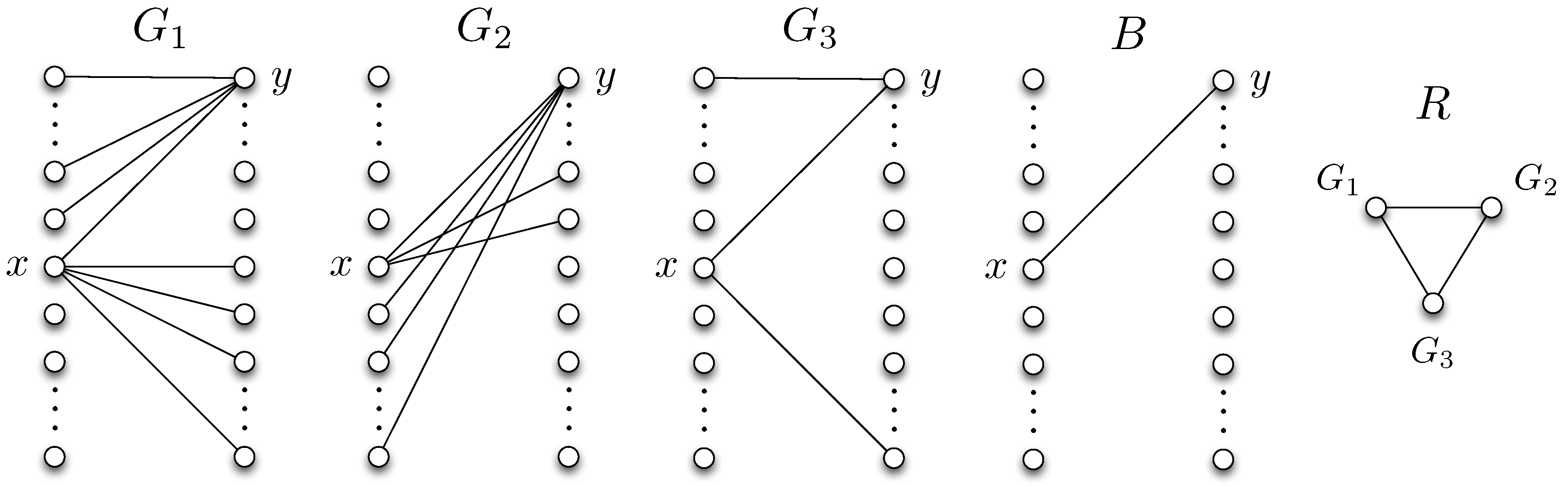
For the reconciliation stage, we first partition Q into groups of distributions with distinct support sets, and denote by B the set of distinct bipartite graphs that correspond to the support sets of the distributions in Q . This process is similar to the one described for P in Section 2.1. Next, we find a lower bound for the minimum number of bits required for user 2 to learn the graph G, i.e., all ( x , y ) pairs that may occur with positive probability under the true distribution p ( x , y ) .
Definition 1.
(Reconciliation graph) Define a characteristic graph R = ( G , E R ) , in which each vertex represents a graph G G . Recall that G is a set of bipartite graphs as we define in Section 2.1. An edge ( G , G ) E R is defined between vertices G and G if and only if there exists a B B such that E B E G and E B E G .
The minimum number of bits required for user 2 to perfectly learn G is then log χ ( R ) , where χ ( · ) denotes the chromatic number of a graph. This can be observed by noting that in the reconciliation phase, any two nodes in the reconciliation graph with an edge in between has to be assigned to distinct bit streams, otherwise user 2 will not be able to distinguish them, which requires a minimum of log χ ( R ) number of bits to be transmitted from user 1 to user 2. It is useful to note that perfect reconciliation incurs a negligible cost for large blocklengths.
Proposition 2.
Perfect reconciliation is an asymptotically optimal strategy.
Proof. 
Since the distributions p ( x , y ) and q ( x , y ) are fixed once chosen, reconciliation requires at most log | R | bits for any class of graphs G . Therefore its contribution on the codeword length per symbol is 1 n log | R | , which vanishes as n . Since the communication cost for not reconciling the graphs can never be lower than reconciling them, we can conclude that reconciling the graphs first, and then using the reconciled graphs for communication, cannot perform worse than not reconciling them. We note, however, that this statement may no longer hold if the joint distribution is arbitrarily varying over the course of n symbols, since correct recovery in this case may require the graphs to be repeatedly reconciled. ☐
In the following, we demonstrate a lower bound on the worst-case message length for this two-stage reconciliation-communication protocol.
Lemma 1.
A lower bound on the worst-case message length for the two-stage reconciliation-communication protocol is,
l R ( n ) log χ ( R ) n + max G G max ( x n , y n ) S G n 1 n log | I G ( x n , y n ) | .
Proof. 
We prove Equation (24) by obtaining a lower bound on the message length for the reconciliation and communication parts separately. The lower bound for the reconciliation part is determined by bounding the minimum number of bits to be transmitted from user 1 to user 2 using Definition 1. As a result, both sides learn the support set of the true distribution p ( x , y ) . The lower bound in Equation (24) then follows from
l R ( n ) log χ ( R ) n + max G G min ϕ max ( x n , y n ) S G n 1 n ( ϕ ( x n , y n ) )
log χ ( R ) n + max G G max ( x n , y n ) S G n min ϕ 1 n ( ϕ ( x n , y n ) )
= log χ ( R ) n + max G G max ( x n , y n ) S G n min ϕ 1 n ( [ ϕ k ( x n , y n ) ] k = 1 r )
log χ ( R ) n + max G G max ( x n , y n ) S G n 1 n log | I G ( x n , y n ) |
where Equation (26) follows from the min-max inequality and Equation (28) from Proposition 1. ☐
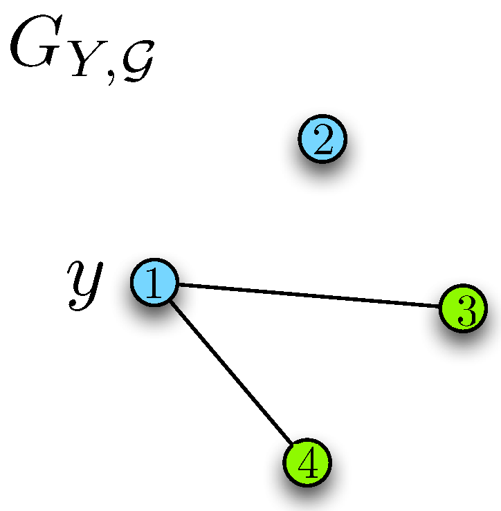
We next demonstrate an upper bound for the minimum worst-case message length. Consider the distribution p ( x , y ) and the corresponding bipartite graph G G . Let G X n = ( X n , E X n ) denote a characteristic graph for user 1 with a vertex set X n . Vertices of G X n are the n-tuples x n X n . An edge ( x n , x ^ n ) E X n exists between x n X n and x ^ n X n whenever some y n Y exists such that ( x n , y n ) S G n , ( x ^ n , y n ) S G n and f n ( x n , y n ) f n ( x ^ n , y n ) . Similarly, define a characteristic graph G Y n = ( Y n , E Y n ) for user 2 whose vertices are the n-tuples y n Y n . An edge ( y n , y ^ n ) E Y n exists between y n Y n and y ^ n Y n whenever some x n X n exists such that ( x n , y n ) S G n , ( x n , y ^ n ) S G n , and f n ( x n , y n ) f n ( x n , y ^ n ) .
The characteristic graphs defined above are useful in that any valid coloring over the characteristic graphs will enable the two parties to resolve the ambiguities in distinguishing the correct function values. 
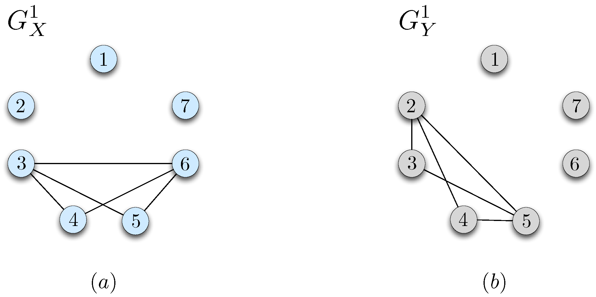
Figure 3 illustrates the characteristic graphs G X 1 and G Y 1 , respectively, constructed by using p 2 ( x , y ) from Equation (20) and f ( x , y ) from Equation (19) in the example discussed in Section 2.2. In the following, we follow the notation G X G X 1 and G Y G Y 1 .
Theorem 1.
The worst-case message length for the two-stage separate reconciliation and communication strategy satisfies
l R ( n ) log χ ( R ) n + max G G 1 n n log ( χ ( G X ) ) + n log ( χ ( G Y ) ) ,
Proof. 
Consider a minimum coloring for G X and G Y using χ ( G X ) and χ ( G Y ) colors. Note that G X n and G Y n can be colored with at most ( χ ( G X ) ) n and ( χ ( G Y ) ) n colors, respectively. Hence, users 1 and 2 can simultaneously send the index of the color assigned to their symbols by using at most n log χ ( G X ) and n log χ ( G Y ) bits, respectively. Then, users can utilize the received color index and their own symbols for correct recovery of the function values. ☐

3.2. Protocols that Do Not Explicitly Start with a Reconciliation Procedure

Instead of the reconciliation-based strategy described in Section 3.1, the two users may choose not to reconcile the distributions, but instead utilize a robust communication strategy that ensures zero-error communication under any distribution in set P . Specifically, they can agree on a worst-case communication strategy that always ensures zero-error communication for both users. In this section, we study two specific protocols that do not explicitly start with a reconciliation procedure. We denote the worst case message length in this setting as l RF ( n ) .
As an example of such a robust communication strategy, consider a scenario in which user 1 enumerates each x n X n by using n log | X | bits whereas user 2 enumerates each y n Y n by using n log | Y | bits. Then, by using no more than n log | X | + n log | Y | bits in total, the two parties can communicate their observed symbols with zero-error under any true distribution, and evaluate f n ( X n , Y n ) . In that sense, this setup does not require any additional bits for learning about the distribution from the other side either perfectly or partially, but the message length for communicating the symbols is often higher. In the following, we derive an upper bound on the worst-case message length based on two achievable protocols that do not start with a reconciliation procedure.
The first achievable strategy we consider is based on graph coloring. Let G X , G = ( X , E X ) be a characteristic graph for user 1 whose vertex set is X . Define an edge ( x , x ^ ) E X between nodes x X and x ^ X whenever there exists some y Y such that ( x , y ) p P supp ( p ) and ( x ^ , y ) p P supp ( p ) whereas f ( x , y ) f ( x ^ , y ) . Similarly, define a characteristic graph G Y , G = ( Y , E Y ) for user 2 whose vertex set is Y . Define an edge ( y , y ^ ) E Y between vertices y Y and y ^ Y whenever there exists some x X such that ( x , y ) supp ( p ) and ( x , y ^ ) supp ( p ) for some p P but f ( x , y ) f ( x , y ^ ) . We note the difference between the conditions for constructing G X , G and G Y , G in that the former is based on the union p P whereas the latter is based on the existence for some p G . This difference results from the fact that user 2 does not know the true distribution, hence needs to distinguish the possible symbols from a group of distributions, whereas user 1 has the true distribution, and can utilize it for eliminating the ambiguities for correct function recovery. We note however that both G X , G and G Y , G depend on G . Lastly, we let χ ( G X , G ) and χ ( G Y , G ) denote the chromatic number of G X , G and G Y , G , respectively.
Then, under any true distribution p P , the following communication protocol ensures zero error. Suppose user 1 observes x n and user 2 observes y n from some distribution p n ( x n , y n ) = i = 1 n p ( x i , y i ) . For each x i X where i = 1 , n , user 1 sends the color of x i by using no more than log χ ( G X , G ) bits. After this step, user 2 can recover f i ( x i , y i ) by using y i as follows. Given y i , user 2 considers the set of all x i X such that p ( x i , y i ) > 0 for some p P . Note that within this set, each color represents a group of x i X for which f i ( x i , y i ) is equal. Therefore, under any true distribution p P , user 2 will be able to recover the correct f i ( x i , y i ) value solely by using the received color along with y i . Similarly, for each y i Y , user 2 sends the color of y i by using no more than log χ ( G Y , G ) bits, after which user 1 recovers f i ( x i , y i ) by using the received color and the true distribution p ( x , y ) . Since user 1 knows the true distribution, it can distinguish any function value correctly as long as no two y , y Y are assigned to the same codeword for which x X such that ( x , y ) supp ( p ) and ( x , y ) supp ( p ) when f ( x , y ) f ( x , y ) .
We then have the following upper bound on the worst-case message length,
l RF ( n ) 1 n n log χ ( G X , G ) + n log χ ( G Y , G ) = log χ ( G X , G ) + log χ ( G Y , G ) bits / symbol ,
where user 1 sends n log ( χ ( G X , G ) ) bits to user 2 whereas user 2 sends n log ( χ ( G Y , G ) ) bits to user 1. After this step, both users can recover the correct function values f n ( x n , y n ) for any source pair ( x n , y n ) supp ( p n ) under any p P .
The second achievable strategy we consider is based on perfect hash functions. A function h : { 1 , , N } { 1 , , k } is called a perfect hash function for a set S { 1 , , N } if for all x , y S such that x y , one has h ( x ) h ( y ) . Define a family of functions H such that h : { 1 , , N } { 1 , , k } for all h H . If
M s ( ln N ) e s 2 / k
for some k s , then, there exists a family of | H | = M functions such that for every S { 1 , , N } with | S | s , there exists a function h H that is injective (one-to-one) over S ([30], Section III.2.3). Perfect hash functions have been proved to be useful for constructing zero-error interactive communication protocols when the true distribution of the sources are known by both parties [7]. In the following, we extend the interactive communication framework from [7] to the setting when the true distribution is unknown by the communicating parties.
Initially, we construct a graph G ¯ ( n ) = ( V , E ) for user 2 with a vertex set V = Y n . In that sense, each vertex of the graph is an n-tuple y n Y n . Define an edge ( y n , y ^ n ) E between vertices y n Y n and y ^ n Y n if for some n-tuple x n X n that there exists some p P for which ( x i , y i ) supp ( p ) and ( x i , y ^ i ) supp ( p ) for all i = 1 , , n . Define a minimum coloring of this graph and let χ ( G ¯ ( n ) ) denote the minimum number of required colors, i.e., the chromatic number of G ¯ ( n ) . In that sense, any valid coloring over this graph will enable user 1 to resolve the ambiguities in distinguishing the correct n-tuple observed by user 2, under any true distribution p P .
We next define the following ambiguity set for each x n X n ,
I X ( x n ) { y n Y n : ( x i , y i ) p P supp ( p ) for i = 1 , , n } ,
as the set of distinct y n sequences that may occur with respect to the support set p P supp ( p ) under the given sequence x n . We denote the size of the largest single-term ambiguity set as,
λ max x X | I X ( x ) | ,
and note that max x n X n | I X ( x n ) | = λ n . Lastly, we define an ambiguity set for each y n Y n ,
I Y ( y n ) { f n ( x n , y n ) F n : x i X and ( x i , y i ) p P supp ( p ) for i = 1 , , n } ,
as the set of distinct function values that may appear for the given sequence y n and with respect to the support set p P supp ( p ) . We denote the size of the largest single-term ambiguity set as
μ max y Y | I Y ( y ) | ,
and note that max y n Y n | I Y ( y n ) | μ n .
The interaction protocol is then given as follows. From Equation (31), there exists a family H of
| H | = λ n ( log χ ( G ¯ ( n ) ) ) e
functions such that h : { 1 , , χ ( G ¯ ( n ) ) } { 1 , , λ 2 n } for all h H and for each S { 1 , , χ ( G ¯ ( n ) ) } of size | S | λ n , there exists an h H that is injective over S . In that sense, the colors assigned to an ambiguity set I X ( x n ) for some x n X n will correspond to some S . Both users initially agree on such a family of functions H and a minimum coloring of graph G ¯ ( n ) with χ ( G ¯ ( n ) ) colors. Suppose user 1 observes x n X n and user 2 observes y n Y n . User 1 finds a function h H that is injective over the colors assigned to vertices y n I X ( x n ) from Equation (32) and sends its index to user 2 by using no more than
log | H | = log λ n ( log χ ( G ¯ ( n ) ) ) e
bits in total. After this step, user 2 evaluates the corresponding function for the assigned color of y n and sends the evaluated value back to user 1 by using no more than log λ 2 n bits. After this step, user 1 will learn the color of y n , from which it can recover y n by using the observed x n . This is due to the fact that from the definition of an ambiguity set I X ( x n ) in Equation (32), every n-tuple y n I X ( x n ) for a given x n X n will receive a different color in the minimum coloring of the graph G ¯ ( n ) . Since the selected perfect hash function is one-to-one over the colors assigned to y n I X ( x n ) , it will allow user 1 to recover the color of y n from the evaluated hash function value. In the last step, user 1 evaluates the function f n ( x n , y n ) , and sends it to user 2 by using no more than log μ n bits. In doing so, she assigns a distinct index for each sequence of function values in the ambiguity set I Y ( y n ) from Equation (34). User 2 can then recover the function f n ( x n , y n ) by using y n and the received index. Overall, this protocol requires no more than
log λ n ( log χ ( G ¯ ( n ) ) ) e + 2 n log λ + n log μ
bits to be transmitted in total, therefore
l NR ( n ) 1 n log λ n ( log χ ( G ¯ ( n ) ) ) e + 2 n log λ + n log μ
1 n log ( λ n ( log χ ( G ¯ ( n ) ) ) e + 1 ) + 2 n log λ + 1 + n log μ + 1
1 n log ( λ n ( log χ ( G ¯ ( n ) ) ) e + 1 ) + 2 n log λ + n log μ + 3
1 n log ( λ n ( log χ ( G ¯ ( n ) ) ) e ) + log 1 + 1 λ n ( log χ ( G ¯ ( n ) ) ) e + 2 n log λ + n log μ + 3
3 log λ + log μ + 1 n log log χ ( G ¯ ( n ) ) + 4 + log e n
3 log λ + log μ + 1 n log n log χ ( G ¯ ( 1 ) ) + 4 + log e n
3 log λ + log μ + 1 n log log χ ( G ¯ ( 1 ) ) + log n n + 4 + log e n
where Equation (42) follows from the fact that 1 λ n ( log χ ( G ¯ ( n ) ) ) e 1 , and Equation (44) holds since χ ( G ¯ ( n ) ) χ n ( G ¯ ( 1 ) ) . This is due to the fact that any coloring over the nth order strong product of G ¯ ( 1 ) is also a valid coloring for G ¯ ( n ) , since by construction of G ¯ ( n ) , any edge that exists in G ¯ ( n ) also exists in the nth order strong product of G ¯ ( 1 ) . Therefore, the chromatic number of G ¯ ( n ) is no greater than the chromatic number of the nth order product of G ¯ ( 1 ) , which is no greater than χ n ( G ¯ ( 1 ) ) .
Combining the bounds obtained from the two protocols from Equations (30) and (45), we have the following upper bound on the worst-case message length.
Proposition 3.
The worst-case message length for the two strategies that do not explicitly start with a reconciliation procedure can be upper bounded as,
l RF ( n ) min log χ ( G X , G ) + log χ ( G Y , G ) , 3 log λ + log μ + 1 n log log χ ( G ¯ ( 1 ) ) + log n n + 4 + log e n .
Proof. 
The result follows from combining the two interaction strategies in Equations (30) and (45). ☐

3.3. Partial Reconciliation

In order to understand the impact of level of reconciliation on the worst-case message length, we consider a third scheme called partial reconciliation, which allows user 2 to distinguish the true distribution up to a class of distributions, after which the two users use a robust worst-case communication protocol that allows for zero-error communication in the presence of any distribution within the class. In that sense, partial reconciliation allows some ambiguity in the reconciled set of distributions. Accordingly, the schemes considered in Section 3.1 and Section 3.2 are special cases of the partial reconciliation scheme. We denote l PR ( n ) as the per-symbol worst-case message length for a finite block of n source symbols under the partial reconciliation scheme. In the following, we demonstrate two protocols for interactive communication with partial reconciliation. The first protocol is based on coloring characteristic graphs, whereas the second protocol is based on perfect hash functions. We then derive an upper bound on the worst-case message length with partial reconciliation.
For the first partial reconciliation protocol, consider the set G of bipartite graphs G = ( X , Y , E G ) constructed by using the distributions p P as described in Section 2.1. Define a partition of the set G as A = { A 1 , A 2 , , A | A | } such that i = 1 | A | A i = G and A i A j = for all i j , where A i is non-empty for i { 1 , , | A | } . Define A ¯ as the set of all such partitions of G .
Fix a partition A A ¯ . For each i { 1 , , | A | } , define a graph G X , A i = ( X , E X ) for user 1 with the vertex set X . Define an edge ( x , x ^ ) E X between nodes x X and x ^ X if there exists some y Y such that ( x , y ) G A i G and ( x ^ , y ) G A i G whereas f ( x , y ) f ( x ^ , y ) . Next, construct a graph G Y , A i = ( Y , E Y ) for user 2 with the vertex set Y . Define an edge ( y , y ^ ) between nodes y Y and y ^ Y if there exists some x X such that ( x , y ) E G and ( x , y ^ ) E G for some G A i but f ( x , y ) f ( x , y ^ ) . Let χ ( G X , A i ) and χ ( G Y , A i ) denote the chromatic number of G X , A i and G Y , A i , respectively.
Then, under any true distribution p P , the following communication protocol ensures zero error. The two users agree on a partition A A ¯ before communication starts. Suppose users 1 and 2 observe x n and y n , respectively, under the true distribution p ( x , y ) . Let G = ( X , Y , E G ) denote the bipartite graph corresponding to the distribution p ( x , y ) . Initially, user 1 sends the index i of the set A i A for which G A i , by using no more than log | A | bits. After this step, user 1 sends the color of each symbol in x n according to the minimum coloring of graph G X , A i by using no more than n log χ ( G X , A i ) bits in total. By using the sequence of colors received from user 1, user 2 can determine the correct function values f n ( x n , y n ) . In the last step, user 2 sends the color of each symbol in y n according to graph G Y , A i by using no more than n log χ ( G Y , A i ) bits. After this step, user 1 can recover the function values f n ( x n , y n ) . Overall, this protocol requires no more than
log | A | + max i { 1 , , | A | } n log χ ( G X , A i ) + log χ ( G Y , A i ) ,
bits to be transmitted. Since one can leverage any partition within A ¯ for constructing the communication protocol, we conclude that the worst-case message length for partial reconciliation is bounded above by,
l PR ( n ) min A A ¯ 1 n log | A | + max i { 1 , , | A | } log χ ( G X , A i ) + log χ ( G Y , A i ) .
For the second partial reconciliation protocol, we again leverage perfect hash functions from Equation (31). As in the first protocol, we define a partition of the set G as A = { A 1 , A 2 , , A | A | } such that i = 1 | A | A i = G and A i A j = for all i j . We let A ¯ be the set of all such partitions of G .
We fix a partition A A ¯ of G . For each i { 1 , , | A | } , we define a graph G ¯ i ( n ) = ( Y n , E ) with the vertex set Y n . We define an edge ( y n , y ^ n ) E between two vertices y n Y n and y ^ n Y n if there exists some x n X n such that ( x j , y j ) G A i E G and ( x j , y ^ j ) G A i E G for j = 1 , , n . We denote the chromatic number of G ¯ i ( n ) by χ ( G ¯ i ( n ) ) .
We define an ambiguity set for each x n X n ,
I i X ( x n ) { y n Y n : ( x j , y j ) G A i E G for j = 1 , , n }
where the size of the largest single-term ambiguity set is given as,
λ i max x X | I i X ( x ) | ,
and note that max x n X n | I i X ( x n ) | λ i n . Next, we define an ambiguity set for each y n Y n ,
I i Y ( y n ) { f n ( x n , y n ) F n : x j X and ( x j , y j ) G A i E G for j = 1 , , n }
and define the size of the largest single-term ambiguity set as,
μ i max y Y | I i Y ( y ) | ,
where max y n Y n | I i Y ( y n ) | μ i n . Given i { 1 , , | A | } , from Equation (31), there exists a family H of
| H | = λ i n ( log χ ( G ¯ i ( n ) ) ) e
functions such that h : { 1 , , χ ( G ¯ i ( n ) ) } { 1 , , λ i 2 n } for all h H and for each S { 1 , , χ ( G ¯ i ( n ) ) } of size | S | λ i n , there exists an h H injective over S . For each i { 1 , , | A | } , the two users agree on a family of functions H and a coloring of graph G ¯ i ( n ) with χ ( G ¯ i ( n ) ) colors. Suppose user 1 observes x n X n and user 2 observes y n Y n . User 1 sends the index of the partition for p to user 2 by using no more than log | A | bits. User 1 then finds a function h H that is injective over the colors of the vertices y n I i X ( x n ) from Equation (49) and sends its index to user 2 by using no more than
log | H | = log λ i n ( log χ ( G ¯ i ( n ) ) ) e
bits. User 2 then evaluates the corresponding function for the assigned color of y n and sends it back to user 1 by using no more than log λ i 2 n bits. After this step, user 1 learns the color of y n , from which it recovers y n by using the observed x n . User 1 then evaluates the function f n ( x n , y n ) , and sends it to user 2 by using no more than log μ i n bits. In doing so, she assigns a distinct index for each sequence of function values in the ambiguity set I i Y ( y n ) from Equation (34). User 2 can then recover the function f n ( x n , y n ) by using y n and the received index. Overall, this protocol requires no more than
log λ i n ( log χ ( G ¯ i ( n ) ) ) e + 2 n log λ i + n log μ i
bits to be transmitted in total, therefore
l PR ( n ) min A A ¯ 1 n log | A | + max i { 1 , , | A | } log λ i n ( log χ ( G ¯ i ( n ) ) ) e + 2 n log λ i + n log μ i
min A A ¯ 1 n log | A | + max i { 1 , , | A | } 3 log λ i + log μ i + 1 n log log χ ( G ¯ i ( 1 ) ) + log n n + 4 + log e n
Combining the bounds obtained from the two protocols in Equations (48) and (57), we have the following upper bound on the worst-case message length with partial reconciliation,
l PR ( n ) min A A ¯ ( 1 n log | A | + min { max i { 1 , , | A | } log χ ( G X , A i ) + log χ ( G Y , A i ) , max i { 1 , , | A | } ( 3 log λ i + log μ i + 1 n log log χ ( G ¯ i ( 1 ) ) + log n n + 4 + log e n ) } ) .
At the outset, partial reconciliation characterizes the interplay between reconciliation and communication costs. In order to understand this inherent reconciliation-communication trade-off, we next identify the cases for which reconciling the missing information is better or worse than not reconciling them. To do so, we provide sufficient conditions under which reconciliation-based strategies can outperform the strategies that do not start with a reconciliation procedure, and vice versa, and show that either strategy can outperform the other. Finally, we demonstrate that partial reconciliation can strictly outperform both.

4. Cases in which Strategies that Do Not Start with a Reconciliation Procedure is Better than Perfect Reconciliation

In this section, we demonstrate that strategies with no explicit reconciliation step can be strictly better than perfect reconciliation.
Proposition 4.
Strategies that do not start with an explicit reconciliation procedure is better than perfect reconciliation if
log χ ( R ) n + max G G max ( x n , y n ) S G n 1 n log | I G ( x n , y n ) | > min log χ ( G X , G ) + log χ ( G Y , G ) , 3 log λ + log μ + 1 n log log χ ( G ¯ ( 1 ) ) + log n n + 4 + log e n .
Proof. 
The result follows from comparing the lower bound on the number of bits required for the perfect reconciliation setting from Equation (24) with the upper bound from Equation (58). ☐
Corollary 1.
Strategies with no explicit reconciliation step can strictly outperform perfect reconciliation.
Proof. 
Consider a scenario in which there exists a parent distribution p * P such that supp ( p ) supp ( p * ) for all p P , then, reconciliation cannot perform better than the strategies with no explicit reconciliation step. This immediately follows from: (i) any zero-error communication strategy for p * is a valid strategy with no explicit reconciliation step, since p P supp ( p ) = supp ( p * ) , (ii) any perfect reconciliation scheme should ensure a valid zero-error communication strategy for p * , as it may appear as the true distribution. Therefore, reconciling distributions cannot decrease the overall message length. Suppose that there exists some q Q for which supp ( q ) supp ( p ) for all p P . Then, Corollary 1 holds whenever | P | > 1 . ☐
We next consider the following example to elaborate on the impact of overlap between the edges of bipartite graphs on the worst-case message length. To do so, we let n = 1 and investigate the following class of graphs.
Definition 2.
(Z-Graph) Consider a class of graphs G for which there exists a single ( x , y ) X × Y such that ( x , y ) E G for all G G . Additionally, assume that for any ( x ^ , y ^ ) X × Y such that ( x ^ , y ^ ) E G for some G G , then either x = x ^ or y = y ^ . In that sense, the structure of these graphs resemble a Z shape, hence we refer to them as Z-graphs. For this class of graphs, λ G = λ G ( x ) and μ G = μ G ( y ) for any G G .
Lemma 2.
Consider the class of graphs defined in Definition 2. For this class of graphs, the worst-case message length for strategies with no explicit reconciliation step satisfies,
l R F ( 1 ) log χ ( G Y , G ) + log μ G
where log χ ( G Y , G ) is defined in Section 3.2 and μ G = max y Y | G G I Y , G ( y ) | such that I Y , G ( y ) is as given in Equation (12).
Proof. 
Consider the following encoding scheme. Group all the neighbors x X of y in G G G that lead to the same function value f ( x , y ) . Assign a single distinct codeword to each of these groups. User 1 sends the corresponding codeword to user 2, which requires no more than log μ G bits, after which user 2 can recover the correct function value. Next, construct the graph G Y , G as defined in Section 3.2. Find the minimum coloring of G Y , G , and assign a distinct codeword to each of the colors. User 2 then sends the corresponding codeword to user 1, by using no more than log χ ( G Y , G ) bits. Note that user 1 can infer the correct function value after this step, as she already knows the bipartite graph G that corresponds to the true distribution and given x and G, each color represents a distinct function value. ☐
Example 1.
Consider the framework of Section 3.1 along with a class of Z-graphs G = { G 1 , G 2 } and B = { B 1 , B 2 } . That is, G 1 , G 2 , B 1 , B 2 share an edge ( x , y ) X × Y such that ( x , y ) E G 1 , E G 2 , E B 1 , E B 2 . Moreover, for any other edge ( x ^ , y ^ ) X × Y , either x ^ = x or y ^ = y . Assume that f ( x , y ) is distinct for each edge ( x , y ) in G . Let
ω | { ( x ^ , y ) : ( x ^ , y ) E G 1 , E G 2 , x ^ X } |
represent the number of common edges, i.e., overlap, between G 1 and G 2 , where 1 ω min { μ G 1 , μ G 2 } . Note that the overlap between G 1 and G 2 can only consist of the edges that share the endpoint y. We consider the following four cases that may occur for the relations between the structures of the graphs G 1 , G 2 , B 1 , B 2 .
  • E B 1 E G 1 , E B 2 E G 1 , E B 1 E G 2 , E B 2 E G 2 . In this case, no reconciliation is always better than reconciliation, because whenever user 2 observes B 1 (respectively B 2 ), he can infer that user 1 knows G 1 (respectively G 2 ).
  • E B 1 E G 1 , E B 2 E G 1 , E B 1 E G 2 , E B 2 E G 2 . In this case, no reconciliation is again optimal as user 2 can infer that user 1 is knows G 1 whenever he observes B 1 or B 2 .
  • E B 1 E G 1 , E B 2 E G 1 , E B 1 E G 2 , E B 2 E G 2 . Then, no reconciliation is again optimal as user 2 can infer that user 1 knows G 2 if she observes B 2 or B 1 .
  • E B 1 E G 1 , E B 2 E G 1 , E B 1 E G 2 , E B 2 E G 2 . In this case, the chromatic number of the reconciliation graph is given by χ ( R ) = 2 from Definition 1. Then the worst-case message length for the perfect reconciliation scheme satisfies,
    l R ( 1 ) 1 + max { log ( λ G 1 + μ G 1 1 ) , log λ G 2 + μ G 2 1 } .
    which follows from Lemma 1. On the other hand, we find that the worst-case message length for the no reconciliation scheme satisfies
    l R F ( 1 ) max { log ( λ G 1 ) , log ( λ G 2 ) } + log ( μ G 1 + μ G 2 ω ) ,
    which follows from Lemma 2 and the following coloring scheme. Suppose max { λ G 1 , λ G 2 } = λ G 1 . Using λ G 1 colors, assign each y ^ Y that is connected to x in G 1 a distinct color. Next, take λ G 2 of these colors excluding the color assigned to node y, and color each y ^ y that is connected to x in G 2 with a distinct color. Note that this is a valid coloring since there are only two bipartite graphs G 1 and G 2 , corresponding to two cliques whose sizes are λ G 1 and λ G 2 in the characteristic graph and the only common node between these two cliques is y. Furthermore, no edge exists across the two cliques. Hence, no reconciliation is better than perfect reconciliation whenever
    max { log λ G 1 , log λ G 2 } + log ( μ G 1 + μ G 2 ω ) < 1 + max { log ( λ G 1 + μ G 1 1 ) , log ( λ G 2 + μ G 2 1 ) } .
    As an example, consider the graphs illustrated in Figure 4 for which λ G 1 = λ G 2 = μ G 1 = μ G 2 = 2 and ω = μ G 1 = μ G 2 . The corresponding characteristic graph and coloring of G Y , G is illustrated in Figure 5. For this case, we observe that no reconciliation is always better than reconciliation.
We note that the performance of a particular communication strategy with respect to others greatly depends on the structure of the partial information as well as the true probability distribution of the observed symbols. In the following section, we show that there exist cases for which reconciling the true distribution only partially can lead to better worst-case message length then both the strategies from Section 3.1 and Section 3.2, indicating that the best communication strategy under partial information may result from a balance between reconciliation and communication costs.

5. Cases in Which Partial Reconciliation is Better

We now investigate the conditions under which partially reconciling the graph information is better than perfect reconciliation. To do so, we initially compare the perfect and partial reconciliation strategies.
Proposition 5.
Partial reconciliation is better than perfect reconciliation if
log χ ( R ) n + max G G max ( x n , y n ) S G n 1 n log | I G ( x n , y n ) | > min A A ¯ ( 1 n log | A | + min { max i { 1 , , | A | } log χ ( G X , A i ) + log χ ( G Y , A i ) , max i { 1 , , | A | } ( 3 log λ i + log μ i + 1 n log log χ ( G ¯ i ( 1 ) ) + log n n + 4 + log e n ) } ) .
Proof. 
The right-hand side of Equation (65) is an upper bound on the zero-error message length with partial reconciliation from Equation (58), whereas the left-hand side lower bounds the zero-error codeword length for perfect reconciliation via Equation (24), from which Equation (65) follows. ☐
We next show that there exist cases for which partial reconciliation strictly outperforms the strategies from Section 3.1 and Section 3.2. To do so, we let n = 1 and again focus on the class of graphs introduced in Definition 2. First, we present an upper bound on the worst-case message length with partial reconciliation for Z-graphs.
Lemma 3.
The worst-case message length with partial reconciliation for the class of graphs from Definition 2 can be upper bounded by,
l P R ( 1 ) min A A ¯ log | A | + max i { 1 , , | A | } log χ ( G Y , A i ) + log μ A i
where log χ ( G Y , A i ) is as defined in Section 3.3 and μ A i = max y Y | G A i I Y , G ( y ) | with I Y , G ( y ) as described in Equation (12).
Proof. 
To prove achievability, note that for a given partition A , at least log | A | bits are necessary for sending the partition index, which reconciles each graph up to the class of graphs in the partition it is assigned to. After reconciliation, zero-error communication requires no more than max i : A i A log χ ( G Y , A i ) + log μ A i in the worst-case. We show this by considering an encoding scheme that ensures zero-error communication for any graph in A i by using log χ ( G Y , A i ) + log μ A i bits. Group all the neighbors x X of y in G A i G that lead to the same function value f ( x , y ) . Assign a single distinct codeword to each of these groups. Note that this requires no more than log μ A i bits in total. Next, for a given partition A i , construct the graph G Y , A i as defined in Section 3.3. Find the minimum coloring of G Y , A i , and assign a distinct codeword to each of the colors, which requires no more than log χ ( G Y , A i ) bits in total. Then, fix a partitioning A of G and use the following communication scheme. User 1, using the partition A , sends the index of the group in which her graph G resides. Then, users 1 and 2 use a robust communication scheme for all the graphs contained in this group. To do so, user 1 sends the codeword assigned to x X by using no more than log μ A i bits, after which user 2 can recover the correct function value. Then, user 2 sends the color assigned to y Y using no more than log χ ( G Y , A i ) bits, after which user 1 can learn the correct function value. ☐
Proposition 6.
Partial reconciliation can strictly outperform the strategies from Section 3.1 and Section 3.2.
Proof. 
Consider the set of Z-graphs G = { G 1 , G 2 , G 3 } and B = { B } in Figure 6. The edge sets satisfy E G 3 E G 1 , E G 2 E G 1 = { ( x , y ) } , and E B = { ( x , y ) } .
Let f ( x , y ) be distinct for each edge ( x , y ) in G , and that λ G i 2 for some i { 1 , 2 } .
First, consider the protocol from Section 3.2. It can be shown that this protocol satisfies
l R F ( 1 ) 1 + log ( μ G 1 + μ G 2 1 )
which results from the following observation. From Proposition 1, it follows that if ( x , y ) , ( x , y ) E G i for some i { 1 , 2 , 3 } , then [ ϕ k X ( x , ϕ k 1 ( x , y ) ) ] k = 1 r cannot be a prefix of [ ϕ k X ( x , ϕ k 1 ( x , y ) ) ] k = 1 r , where [ ϕ k X ( x , ϕ k 1 ( x , y ) ) ] k = 1 r is the sequence of bits sent by user 1 in r rounds. Next, suppose that for some ( x , y ) E G i and ( x , y ) E G j where i j , and [ ϕ k X ( x , ϕ k 1 ( x , y ) ) ] k = 1 r is a prefix of [ ϕ k X ( x , ϕ k 1 ( x , y ) ) ] k = 1 r . Since user 2 does not know the true distribution, she cannot distinguish between x and x , causing an error since ( x , y ) and ( x , y ) lead to different function values. This in turn violates the zero-error condition. As a result, [ ϕ k X ( x , ϕ k 1 ( x , y ) ) ] k = 1 r should be prefix free for all x I Y ( y ) defined in Equation (34) whose size is μ G 1 + μ G 2 1 . Therefore, user 1 needs to send at least log ( μ G 1 + μ G 2 1 ) bits to user 2. Next, we demonstrate that user 2 needs to send at least 1 bit to user 1. Suppose that this is not true, i.e., user 2 does not send anything. Since λ G i 2 for some i { 1 , 2 } , in this case user 1 will not be able to distinguish between two distinct function values for at least one graph that may occur at user 1. Therefore, by contradiction, Equation (67) provides a lower bound for Z-graphs for the protocols that do not start with a reconciliation strategy considered in Section 3.2.
Next, consider the perfect reconciliation protocol. For this scheme, we construct the reconciliation graph R as given in Figure 6, and observe that any encoding strategy that allows user 2 to distinguish the graph of user 1 requires 3 colors (distinct codewords). After this step, both users consider one of G 1 , G 2 , or G 3 . Then,
l R ( 1 ) log 3 + max G i G log ( λ G i + μ G i 1 )
which follows from Lemma 1 with the observation that | I G i ( x , y ) | = λ G i + μ G i 1 for i { 1 , 2 , 3 } .
Lastly, consider the partial reconciliation protocol. In particular, consider a partial reconciliation scheme achieved by the partitioning A = { A 1 , A 2 } such that A 1 = { G 1 , G 3 } , and A 2 = { G 2 } . Then, from Equation (66), we obtain
l P R ( 1 ) log 2 + max { log λ G 1 + log μ G 1 , log λ G 2 + log μ G 2 } .
Therefore, whenever λ G 1 , λ G 2 , μ G 1 , μ G 2 satisfy
log 2 + max { log λ G 1 + log μ G 1 , log λ G 2 + log μ G 2 } < 1 + log ( μ G 1 + μ G 2 1 ) ,
then, partial reconciliation outperforms the strategies from Section 3.2. On the other hand, whenever λ G 1 , λ G 2 , μ G 1 , μ G 2 satisfy
log 2 + max { log λ G 1 + log μ G 1 , log λ G 2 + log μ G 2 } < log 3 + max { log ( λ G 1 + μ G 1 1 ) , log ( λ G 2 + μ G 2 1 ) } ,
then, partial reconciliation outperforms the perfect reconciliation scheme. By setting λ G 1 = 2 , μ G 1 = 8 , λ G 2 = 1 , μ G 2 = 16 , we observe that l P R ( 1 ) 5 whereas l R ( 1 ) 6 and l R F ( 1 ) 6 and both Equations (70) and (71) are satisfied, from which Proposition 6 follows. ☐
Therefore, under certain settings, it is strictly better to design the interaction protocols to allow the communicating parties to agree on the true source distribution only partially, than to learn it perfectly or not learn it at all, pointing to an inherent reconciliation-communication tradeoff.

6. Communication Strategies with Symmetric Priors

In this section we let P = Q and | P | = 1 and specialize the communication model to the conventional function computation scenario where the true distribution p ( x , y ) of the sources is known by both users. Users thus share a common bipartite graph G = ( X , Y , E ) which they can leverage for interactive communication. We first state a simple lower bound on the worst-case message length.
Proposition 7.
A lower bound on the worst-case message length when the true distribution is known by both parties is,
l ( n ) max ( x n , y n ) S G n 1 n log | I G ( x n , y n ) | .
Proof. 
For the worst-case codeword length, we have
l ( n ) = min ϕ max ( x n , y n ) S G n 1 n ( ϕ ( x n , y n ) )
max ( x n , y n ) S G n min ϕ 1 n ( ϕ ( x n , y n ) )
max ( x n , y n ) S G n 1 n log | I G ( x n , y n ) |
where Equation (74) follows from the min-max inequality whereas Equation (75) follows from Proposition 1. ☐
We next consider the upper bounds on the worst-case message length for this scenario. A simple upper bound can be obtained via the graph coloring approach in Theorem 1,
l ( n ) 1 n n log ( χ ( G X ) ) + n log ( χ ( G Y ) ) ,
where the characteristic graphs G X and G Y are constructed as in Theorem 1 using the bipartite graph corresponding to the true distribution p ( x , y ) . We note that Equation (76) implies that
lim n l ( n ) log ( χ ( G X ) ) + log ( χ ( G Y ) ) .
The above approach may yield limited gains for compression for large values of χ ( G X ) and χ ( G Y ) , and another round of interaction may help reduce the compression rate. We next provide another upper bound that combines graph coloring and hypergraph partitioning. To do so, we first review the following notable results. The first one is a technical result regarding partitioning hypergraphs.
Lemma 4 ([1]).
Define Γ = ( V , E ) to be a hypergraph with a vertex set of size | V | , and the hyperedges E m V with m = 1 , , | E | . Assume that each hyperedge has at most κ elements, i.e., | E m | κ . Then for any given ϵ > 0 , there exists a constant ρ ( ϵ ) such that s ( ln | V | | E | ) 1 + ϵ and s > 1 , a partition V 1 , V 2 , V κ s ρ ( ϵ ) of V can be found with | V k E m | < s for all m = 1 , , | E | and k = 1 , , κ s ρ ( ϵ ) .
We can now state the second useful result.
Lemma 5 ([1]).
The following worst-case codeword length can be achieved in three rounds for n = 1 ,
l ( 1 ) log Δ X + log Δ Y + ( 1 + ϵ ) log log | X | | Y | + 2 log ρ ( ϵ ) + 5 .
where each person makes two non-empty transmissions.
We next derive an upper bound based on Lemma 5 by increasing the number of interaction rounds and following a sequential hypergraph partitioning approach. This allows the proposed scheme to work in low-rate communication environments when parties do not mind having extra rounds of interaction.
Theorem 2.
Given a joint probability distribution p ( x , y ) , consider the corresponding bipartite graph G = ( X , Y , E ) . Consider a partition of X n into Δ Y n ( ln | X n | | Y n | ) 1 + ϵ ρ ( ϵ ) groups such that for each group X u n ,
| X u n x n : ( x n , y n ) S n , x n X n | ( ln | X n | | Y n | ) 1 + ϵ , y n Y n ,
where u = 1 , , min { Δ X n , Δ Y n } ( n ln | X | | Y | ) 1 + ϵ ρ ( ϵ ) . Then, the worst-case codeword length with four total rounds can be bounded by using sequential hypergraph partitioning as
l ( n ) log Δ X + log Δ Y + ( 1 + ϵ ) n log log γ n + 2 n log ρ ( ϵ ) + 5 n
where γ n = max u | X u n | × min { Δ X n | X u n | , | Y n | } | X | n | Y | n .
Proof. 
Our proof builds upon [1] as follows. The set of symbols in the first round are from X n and Y n for users 1 and 2, respectively. We assume Δ X > Δ Y without loss of generality. Let s 1 = ( ln | X n | | Y n | ) 1 + ϵ . From Lemma 4, X n can be partitioned into Δ Y n s 1 ρ ( ϵ ) groups such that for each group X u n ,
| X u n x n : ( x n , y n ) S n , x n X n | s 1 , y n Y n ,
where u = 1 , , Δ Y n s 1 ρ ( ϵ ) . In this round, user 1 sends the index of the group that her symbol resides in by using no more than log ( Δ Y n s 1 ρ ( ϵ ) ) bits, and user 2 makes a null transmission. Let u ^ be the index of the group sent by user 1 in the first round. In the second round, the following set is considered by user 2 after receiving the index from user 1
Y u ^ n = y n : ( x n , y n ) S n , x n X u ^ n , y n Y n .
Note that | Y u ^ n | min { Δ X n | X u ^ n | , | Y n | } . Next, consider a hypergraph Γ = ( V , E ) with the vertex set V = Y u ^ n and define a hyperedge for each x n X u ^ n as follows.
E x n = { y n : ( x n , y n ) S n , y n Y u ^ n } ,
where | E | = | X u ^ n | , and | E x n | Δ X n , x n X u ^ n . User 1 can also determine this set by using the group index for her symbol and the relations between the function values of both parties. Let
s 2 u ^ = ln | V | | E | 1 + ϵ = ln | Y u ^ n | | X u ^ n | 1 + ϵ s 1 .
User 2 then partitions Y u ^ n into Δ X n s 2 u ^ ρ ( ϵ ) groups and sends the group index for his symbol, which requires no more than log ( Δ X n s 2 u ^ ρ ( ϵ ) ) bits. After receiving the group index, user 1 has to decide from at most s 2 u ^ possible symbols from user 2.
In the third round, symbols are now restricted to a subspace of X n × Y n with at most s 1 possible symbols from user 1 for each symbol from user 2 and at most s 2 u ^ possible symbols from user 2 for each one of the symbols of user 1. Then, by using ([1], Lemma 2), one can find that no more than log ( s 1 ) + 2 log ( s 2 u ^ ) bits are required.
This scheme requires four rounds of interaction in total; each person makes two non-empty transmissions. The total number of bits required in the worst-case satisfies
l ( n ) 1 n max u log Δ Y n s 1 ρ ( ϵ ) + log Δ X n s 2 u ρ ( ϵ ) + log s 1 + 2 log s 2 u
1 n max u log Δ Y n + log Δ X n + log s 2 u + 2 log ρ ( ϵ ) + 5
log Δ X + log Δ Y + 1 n ( 1 + ϵ ) log log γ n + 2 log ρ ( ϵ ) + 5 ,
where γ n = max u | X u n | | Y u n | | X | n | Y | n . ☐
Corollary 2.
In the limit of large block lengths, the upper bound of Theorem 2 satisfies
lim n l ( n ) = log Δ X + log Δ Y .
Proof. 
As | X u n | | X n | and | Y u n | | Y n | for all partitions u of X n and Y n , from Theorem 2,
lim n l ( n ) lim n log Δ X + log Δ Y + ( 1 + ϵ ) n log log | X | | Y | + ( 1 + ϵ ) log n n + 2 n log ρ ( ϵ ) + 5 n = log Δ X + log Δ Y .
 ☐
Lemma 5 and Theorem 2 apply the hypergraph partitioning technique to the bipartite graph of the joint distribution p ( x , y ) , but provide achievable rates by first performing source reconstruction at the two ends, after which both users can compute the correct function value. The next theorem takes the function values into account while constructing the hypergraph partitioning algorithm, with the use of characteristic graphs.
Consider any valid coloring of the characteristic graphs G X n and G Y n defined in Section 3.1. Note that by using their own symbols, each user can recover the correct function values upon receiving the color from the other user. The problem now reduces to sharing the colors between the two parties correctly, for which we apply sequential hypergraph partitioning to the colors of the graphs G X n and G Y n .
Theorem 3.
Define a coloring α : G X n C α for G X n with | C α | colors, and a coloring β : G Y n C β for G Y n with | C β | colors. Let c ( x n ) and c ( y n ) denote the colors assigned to x n and y n by the colorings α and β, respectively. Define the ambiguity set for color c X C α as
J X ( c X ) { c Y C β : ( x n , y n ) S n , c ( x n ) = c X , c ( y n ) = c Y }
with the size bound Δ X α ( n ) max c X C α | J X ( c X ) | , and the ambiguity set for color c Y C β as
J Y ( c Y ) { c X C α : ( x n , y n ) S n , c ( x n ) = c X , c ( y n ) = c Y }
with the size bound Δ Y β ( n ) max c Y C β | J Y ( c Y ) | . Consider a partition of C α into min { Δ X α ( n ) , Δ Y β ( n ) } ( ln | C α | | C β | ) 1 + ϵ ρ ( ϵ ) groups such that for each group C α u ,
| C α u J Y ( c Y ) | ln | C α | | C β | 1 + ϵ c Y C β ,
and
C β u { c Y C β : ( x n , y n ) S n , c ( x n ) = c X C α u , c ( y n ) = c Y } .
where u = 1 , , min { Δ X α ( n ) , Δ Y β ( n ) } ( ln | C α | | C β | ) 1 + ϵ ρ ( ϵ ) . Then, the worst-case message length can be upper bounded as,
l ( n ) min α , β log Δ X α ( n ) n + log Δ Y β ( n ) n + ( 1 + ϵ ) n log log γ α , β + 2 n log ρ ( ϵ ) + 5 n ,
where γ α , β = max u | C α u | | C β u | .
Proof. 
Assume Δ X α ( n ) > Δ Y β ( n ) without loss of generality. Choose s 1 = ( ln | C α | | C β | ) 1 + ϵ . Partition C α into Δ Y β ( n ) s 1 ρ ( ϵ ) groups such that in each partition the number of colors from the ambiguity set is no greater than s 1 . Hence, for any c Y C β ,
| C α u { c X : ( x n , y n ) S n , c ( x n ) = c X C α , c ( y n ) = c Y } | s 1 ,
for u = 1 , , Δ Y α ( n ) s 1 ρ ( ϵ ) . In the first round, user 1 sends the index of the partition the color of her symbols lies in. This requires at most log ( Δ Y β ( n ) s 1 ρ ( ϵ ) ) bits, whereas user 2 makes an empty transmission. Denote u ^ as the index of the partition sent from user 1. In the second round, upon receiving u ^ from user 1, user 2 considers a set C β u ^ given as u = u ^ in Equation (93), where | C β , u ^ | min { λ ˜ m a x | C α u ^ | , | C β | } . Define a hypergraph Γ = ( V , E ) with a vertex set V = C β u ^ and a hyperedge E c X = { c Y : ( x n , y n ) S n , c ( y n ) = c Y C β u ^ , c ( x n ) = c X } for each c X C α u ^ such that | E | = | C α u ^ | , and | E c X | Δ X α ( n ) for every c X C α u ^ . Define s 2 u ^ = ( ln | V | | E | ) 1 + ϵ = ( ln | C β u ^ | | C α u ^ | ) 1 + ϵ < s 1 and partition C β u ^ into Δ X α ( n ) s 2 u ^ ρ ( ϵ ) to groups so that user 2 can send the index of his symbols with at most log ( Δ X α ( n ) s 2 u ^ ρ ( ϵ ) ) bits. Upon receiving the index, user 1 can reduce the number of possible symbols from user 2 to at most s 2 u ^ . Colors in the third round are restricted to a subset of C α × C β such that for every color from user 1 (user 2), there are at most s 2 u ^ ( s 1 ) possible colors exist from user 2 (user 1). Then Equation (94) follows from ([1], Lemma 2).
It can be observed from Equation (94) that different codeword lengths are obtained by different colorings, since they lead to different color and ambiguity set sizes. In general, there exists a trade-off between the ambiguity set sizes and the number of colors, such that using a smaller number of colors may in turn increase the ambiguity set sizes. The exact nature of the bound depends on the graphical structures such as degree and connectivity, however, any valid coloring allows error-free recovery. For instance, assigning a distinct color to each element of X n and Y n is a valid coloring scheme. If one restricts oneself to such set of colorings, the coding scheme of Theorem 3 will reduce to that of Theorem 2, hence the bound in Theorem 3 generalizes the achievable protocols in Theorem 2.

7. Conclusions

In this paper, we have considered a communication scenario in which two parties interact to compute a function of two correlated sources with zero error. The prior distribution available at one of the communicating parties is possibly different from the true distribution of the sources. In this setting, we have studied the impact of reconciling the missing information about the true distribution prior to communication on the worst-case message length. We have identified sufficient conditions under which reconciling the partial information is better or worse than not reconciling it but instead using a robust communication protocol that ensures zero-error recovery despite the asymmetry in the knowledge of the distribution. Accordingly, we have provided upper and lower bounds on the worst-case message length for computing multiple descriptions of the given function. Our results point to an inherent reconciliation-communication tradeoff, in that an increased reconciliation cost often leads to a lower communication cost. A number of interesting future directions remain. In this paper, we do not consider additional strategies which consider further information that may be revealed by the function realizations on the support set. Developing interaction strategies that leverage this information is another interesting future direction. A second one is finding the optimal joint reconciliation-communication strategy in general and the study of alternative upper bounds that take into account the specific structure of the function and input distributions. Another interesting direction is to model the case where knowledge asymmetry is due to one party having superfluous information.

Acknowledgments

This research was sponsored by the U.S. Army Research Laboratory and was accomplished under Cooperative Agreement Number W911NF-09-2-0053 (the ARL Network Science CTA). The views and conclusions contained in this document are those of the authors and should not be interpreted as representing the official policies, either expressed or implied, of the Army Research Laboratory or the U.S. Government. The U.S. Government is authorized to reproduce and distribute reprints for Government purposes notwithstanding any copyright notation here on. Earlier versions of this work have partially appeared at the IEEE GlobalSIP Symposium on Network Theory, December 2013, IEEE Data Compression Conference (DCC’14), March 2014, and IEEE Data Compression Conference (DCC’16), March 2016. This document does not contain technology or technical data controlled under either the U.S. International Traffic in Arms Regulations or the U.S. Export Administration Regulations.

Author Contributions

The ideas in this work were formed by the discussions between Basak Guler and Aylin Yener with Prithwish Basu and Ananthram Swami. Basak Guler is the main author of the paper.

Conflicts of Interest

The authors declare no conflict of interest.

References

  1. El Gamal, A.; Orlitsky, A. Interactive data compression. In Proceedings of the IEEE Symposium on Foundations of Computer Science (FOCS’84), West Palm Beach, FL, USA, 24–26 October 1984; pp. 100–108. [Google Scholar]
  2. Orlitsky, A. Worst-case interactive communication I: Two messages are almost optimal. IEEE Trans. Inf. Theory 1990, 36, 1111–1126. [Google Scholar] [CrossRef]
  3. Guler, B.; Yener, A.; Basu, P. A study of semantic data compression. In Proceedings of the IEEE Global Conference on Signal and Information Processing (GlobalSIP’13), Austin, TX, USA, 3–5 December 2013; pp. 887–890. [Google Scholar]
  4. Guler, B.; Yener, A. Compressing semantic information with varying priorities. In Proceedings of the IEEE Data Compression Conference (DCC’14), Snowbird, UT, USA, 26–28 March 2014; pp. 213–222. [Google Scholar]
  5. Yao, A.C. Some complexity questions related to distributed computing. In Proceedings of the 11th Annual ACM Symposium on Theory of Computing (STOC’79), Atlanta, GA, USA, 30 April–2 May 1979; pp. 209–213. [Google Scholar]
  6. Feder, T.; Kushilevitz, E.; Naor, M.; Nisan, N. Amortized communication complexity. SIAM J. Comput. 1995, 24, 736–750. [Google Scholar] [CrossRef]
  7. Kushilevitz, E.; Nisan, N. Communication Complexity; Cambridge University Press: Cambridge, UK, 1997. [Google Scholar]
  8. Orlitsky, A.; Roche, J.R. Coding for computing. IEEE Trans. Inf. Theory 2001, 47, 903–917. [Google Scholar] [CrossRef]
  9. Ma, N.; Ishwar, P. Some results on distributed source coding for interactive function Computation. IEEE Trans. Inf. Theory 2011, 57, 6180–6195. [Google Scholar] [CrossRef]
  10. Ma, N.; Ishwar, P.; Gupta, P. Interactive source coding for function computation in collocated networks. IEEE Trans. Inf. Theory 2012, 58, 4289–4305. [Google Scholar] [CrossRef]
  11. Yang, E.H.; He, D.K. Interactive encoding and decoding for one way learning: Near lossless recovery with side information at the decoder. IEEE Trans. Inf. Theory 2010, 56, 1808–1824. [Google Scholar] [CrossRef]
  12. Shannon, C. The zero error capacity of a noisy channel. IRE Trans. Inf. Theory 1956, 2, 8–19. [Google Scholar] [CrossRef]
  13. Witsenhausen, H.S. The zero-error side information problem and chromatic numbers. IEEE Trans. Inf. Theory 1976, 22, 592–593. [Google Scholar] [CrossRef]
  14. Simonyi, G. On Witsenhausen’s zero-error rate for multiple sources. IEEE Trans. Inf. Theory 2003, 49, 3258–3260. [Google Scholar] [CrossRef]
  15. Körner, J. Coding of an information source having ambiguous alphabet and the entropy of graphs. In Proceedings of the Sixth Prague Conference on Information Theory, Prague, Czech Republic, 19–25 September 1973; pp. 411–425. [Google Scholar]
  16. Alon, N.; Orlitsky, A. Source coding and graph entropies. IEEE Trans. Inf. Theory 1995, 42, 1329–1339. [Google Scholar] [CrossRef]
  17. Doshi, V.; Shah, D.; Médard, M.; Effros, M. Functional compression through graph coloring. IEEE Trans. Inf. Theory 2010, 56, 3901–3917. [Google Scholar] [CrossRef]
  18. Minsky, Y.; Trachtenberg, A.; Zippel, R. Set reconciliation with nearly optimal communication complexity. IEEE Trans. Inf. Theory 2003, 49, 2213–2218. [Google Scholar] [CrossRef]
  19. Nayak, J.; Rose, K. Graph capacities and zero-error transmission over compound channels. IEEE Trans. Inf. Theory 2005, 51, 4374–4378. [Google Scholar] [CrossRef]
  20. Berners-Lee, T.; Hendler, J.; Lassila, O. The semantic Web. Sci. Am. 2001, 284, 28–37. [Google Scholar] [CrossRef]
  21. Sheth, A.; Bertram, C.; Avant, D.; Hammond, B.; Kochut, K.; Warke, Y. Managing semantic content for the Web. IEEE Internet Comput. 2002, 6, 80–87. [Google Scholar] [CrossRef]
  22. Lee, E.A. Cyber physical systems: Design challenges. In Proceedings of the IEEE International Symposium on Object Oriented Real-Time Distributed Computing (ISORC’08), Orlando, FL, USA, 5–7 May 2008; pp. 363–369. [Google Scholar]
  23. Sheth, A.; Henson, C.; Sahoo, S. Semantic sensor Web. IEEE Internet Comput. 2008, 12, 78–83. [Google Scholar] [CrossRef]
  24. Chen, J.; He, D.K.; Jagmohan, A. On the duality between Slepian–Wolf coding and channel coding under mismatched decoding. IEEE Trans. Inf. Theory 2009, 55, 4006–4018. [Google Scholar] [CrossRef]
  25. Juba, B.; Kalai, A.T.; Khanna, S.; Sudan, M. Compression without a common prior: An information-theoretic justification for ambiguity in language. In Proceedings of the Second Symposium on Innovations in Computer Science (ICS 2011), Beijing, China, 7–9 January 2011. [Google Scholar]
  26. Haramaty, E.; Sudan, M. Deterministic compression with uncertain priors. Algorithmica 2016, 76, 630–653. [Google Scholar] [CrossRef]
  27. Guler, B.; Yener, A.; MolavianJazi, E.; Basu, P.; Swami, A.; Andersen, C. Interactive Function Compression with Asymmetric Priors. In Proceedings of the IEEE Data Compression Conference (DCC’16), Snowbird, UT, USA, 30 March–1 April 2016; pp. 379–388. [Google Scholar]
  28. Cover, T.M.; Thomas, J.A. Elements of Information Theory; John Wiley & Sons: Hoboken, NJ, 2012. [Google Scholar]
  29. Gács, P.; Körner, J. Common information is far less than mutual information. Probl. Control Inf. Theory 1973, 2, 149–162. [Google Scholar]
  30. Mehlhorn, K. Data Structures and Algorithms 1: Sorting and Searching; Springer Science & Business Media: Berlin, Germany, 2013. [Google Scholar]
Figure 1. Bipartite graph representation of the probability distribution from Equation (17). Edge labels represent the function values f ( x , y ) = ( x + y ) mod 4 . Note that the maximum vertex degree is Δ X = 3 for x X and Δ Y = 5 for y Y whereas λ G = 3 and μ G = 4 .
Entropy 19 00635 g001
Figure 2. Shared bipartite graph with n = 1 . X = Y = { 1 , , 7 } representing the distribution p 2 ( x , y ) from Equation (20). Edge labels represent the function values f ( x , y ) defined in Equation (19). Maximum vertex degrees are Δ X = Δ Y = 4 for x X and y Y whereas λ G = μ G = 3 .
Entropy 19 00635 g002
Figure 3. Characteristic graphs (a) G X 1 and (b) G Y 1 constructed using distribution p 2 ( x , y ) in Equation (20) and function f ( x , y ) in Equation (19).
Entropy 19 00635 g003
Figure 4. Example graphs G = { G 1 , G 2 } and B = { B 1 , B 2 } , where λ G 1 = λ G 2 = μ G 1 = μ G 2 = 2 .
Entropy 19 00635 g004
Figure 5. Coloring of the characteristic graph G Y , G .
Entropy 19 00635 g005
Figure 6. Bipartite graphs G = { G 1 , G 2 , G 3 } , B = { B } , and the corresponding reconciliation graph R.
Entropy 19 00635 g006

