Article

Cosine Similarity Entropy: Self-Correlation-Based Complexity Analysis of Dynamical Systems

Department of Electrical and Electronic Engineering, Imperial College, SW7 2AZ London, UK
*
Author to whom correspondence should be addressed.
Entropy 2017, 19(12), 652; https://doi.org/10.3390/e19120652
Submission received: 24 October 2017 / Revised: 20 November 2017 / Accepted: 27 November 2017 / Published: 30 November 2017
(This article belongs to the Special Issue Information Theory Applied to Physiological Signals)

Abstract

:
The nonparametric Sample Entropy (SE) estimator has become a standard for the quantification of structural complexity of nonstationary time series, even in critical cases of unfavorable noise levels. The SE has proven very successful for signals that exhibit a certain degree of the underlying structure, but do not obey standard probability distributions, a typical case in real-world scenarios such as with physiological signals. However, the SE estimates structural complexity based on uncertainty rather than on (self) correlation, so that, for reliable estimation, the SE requires long data segments, is sensitive to spikes and erratic peaks in data, and owing to its amplitude dependence it exhibits lack of precision for signals with long-term correlations. To this end, we propose a class of new entropy estimators based on the similarity of embedding vectors, evaluated through the angular distance, the Shannon entropy and the coarse-grained scale. Analysis of the effects of embedding dimension, sample size and tolerance shows that the so introduced Cosine Similarity Entropy (CSE) and the enhanced Multiscale Cosine Similarity Entropy (MCSE) are amplitude-independent and therefore superior to the SE when applied to short time series. Unlike the SE, the CSE is shown to yield valid entropy values over a broad range of embedding dimensions. By evaluating the CSE and the MCSE over a variety of benchmark synthetic signals as well as for real-world data (heart rate variability of three different cardiovascular pathologies), the proposed algorithms are demonstrated to be able to quantify degrees of structural complexity in the context of self-correlation over small to large temporal scales, thus offering physically meaningful interpretations and rigor in the understanding the intrinsic properties of the structural complexity of a system, such as the number of its degrees of freedom.

1. Introduction

Entropy-based structural complexity assessment is one of the most important nonlinear analysis tools for quantifying degrees of freedom in signals and systems, especially for time series. A well-known statistical entropy method, called Approximate Entropy (ApEn) [1,2], has been developed particularly for the analysis of physiological signals, such as heart rate variability (HRV). Such an approach is based on the statistics of occurrences of similar patterns in a time series. These are found in reconstructed elements, so-called embedding vectors, which preserve the underlying dynamical properties of the system when an appropriate embedding dimension (m) and time lag ( τ ) are chosen [3,4,5]. The Sample Entropy (SE) estimator, proposed by [6], is an improved version of the ApEn, whereby the occurrences of the self-similar patterns are not considered; this results in unbiased entropy estimates; this enhanced robustness has made the SE algorithm become an extremely popular in practical applications. However, despite considerable success, there exist some limitations of the SE which are related to: (i) a short length of sample size; (ii) spikes or erratic noise in data; and (iii) unconstrained entropy values (no bounds).
To provide insight into these limitations and outline the proposed solutions, it is important to notice that, in the SE approach, entropy is estimated based on conditional probability, whereby the probability of occurrences of similar patterns found in the embedding vectors with a dimension (m) is compared to the probability of the occurrences of similar patterns found in the embedding vectors with an enlarged dimension ( m + 1 ) , defined as a reference frame. This method is effective when a time series has sufficiently many samples ( 10 m to 30 m as a rule of thumb [7]); however, for short time series (the first issue above), undefined entropy values can arise due to the convergence in probability to zero; i.e., few occurrences of similar patterns are found in embedding vectors with the dimension of either m or ( m + 1 ) [8]. Regarding the second issue, since the assessment of the similarity in the SE is based on the amplitude-based distance called the Chebyshev distance, spurious peaks or high amplitude of spikes (which typically present in real world data, such as in QRS complexes of Electrocardiograms (ECG), epileptic seizures in Electroencephalograms (EEG), movement artifacts, or any failures of recording devices or of sensors [9]) present in a time series directly affect such a distance metric and consequently alter the number of occurrences of similar patterns found in the embedding vectors for both the dimensions m and ( m + 1 ) ; this results in either a reduction or increase in entropy values [9,10] and suggests that rapid changes in amplitudes cause inconsistent entropy estimates. Furthermore, estimation of entropy is based on the natural logarithm that gives an uncontrollable range of entropy values for small values of the proxy for the probability within the algorithm (the third issue above). To this end, the recent Fuzzy Entropy (FE), an improved version of the sample entropy has been proposed in [11,12,13,14,15] in order to provide more robust examination of the similarity between embedding vectors. This is achieved by replacing the Heaviside function (or a hard threshold), used as a criterion in the SE, with a fuzzy membership function, such as a Sigmoid or Gaussian ones. The FE has been proven to be superior to the SE for short sample sizes and is robust to spikes in data [11]. However, the SE and FE yield different entropy estimates (for sufficient samples), whereby the FE yields both lower entropy values and their variation (standard deviation) than the entropy calculated from the standard SE.
It is important to notice that the SE behaves monotonically with respect to the degrees of uncertainty or, in other words, the higher the randomness, the greater the entropy. This implies that the SE is effectively a tool for quantifying degrees of uncertainty-based complexity [6,16,17]. However, completely random signals have no structure and are therefore not complex, and structural complexity should be considered in the context of (self) correlation over small to large temporal scales, such as in coarse-grained scales employed in the Multiscale Sample Entropy (MSE) algorithm, proposed in [18,19,20,21]. Indeed, it is the MSE that made a significant step forward in the way we understand and deal with complexity of real-world data. An illustrative example of the complexity analysis using the MSE is a comparison of a long-term correlated pink noise signal ( 1 / f , fractal behavior with a tremendous amount of structure) and uncorrelated random noise [20]. Random noise at the smallest scale factor (standard entropy) has a higher entropy than the entropy of the truly complex self-similar and infinitely repeating 1 / f noise. However, with an increase in the scale factor, the entropy of random noise decreases owing to no structure in white noise, while the entropy of the 1 / f noise remains constant over the whole range of scale factors. Therefore, at the largest scale factor (long-term correlation), the entropy of random noise reduces dramatically and is lower than that of the 1 / f noise; the implication of this result is the requirement for the quantification of complexity based on self-correlation over small to large scale factors, as emphasized in this study.
The algorithms proposed here are called the “Cosine Similarity Entropy” (CSE), with its extended multiscale version called the “Multiscale Cosine Similarity Entropy” (MCSE), and are based on fundamental modifications of the SE and the MSE approaches, which makes the CSE amplitude-independent and robust to spikes and short length of data segments, two key problems with the standard SE. First, Shannon entropy is employed instead of the conditional entropy owing to its rigorous properties: (i) anti-monotonicity (an increase in entropy with a decrease in probability and vice versa); (ii) for a uniform distribution of probability, it exhibits a unique maximum entropy; and (iii) entropy is zero only if the probability is 1 (no new information) [22]. In terms of a distance metric, we employ the angular distance, a family of the cosine similarity metrics, which is an amplitude-independent distance. The angular distance used is shown to comply with the four axioms of the distance in metric spaces: (i) non-negativity; (ii) identity for indiscernibles; (iii) symmetry; and (iv) triangle inequality [23,24]. To illustrate the concept, we examine the characteristics of CSE over varying tolerance levels for four benchmark synthetic signals: (i) white Gaussian noise, (ii) 1 / f noise, (iii) first order autoregressive model, autoregressive processes AR(1), and (iv) second order autoregressive model, AR(2). For rigor, the effects of different embedding dimensions and sample sizes on the SE, FE and CSE approaches are investigated, while, for the multiscale CSE approach, the performances of the corresponding multiscale versions, MCSE, MSE and the multiscale fuzzy entropy (MFE) are assessed by evaluating the complexity profiles of these four characteristic synthetic signals over a range of scales. Finally, the effectiveness of the three multiscale approaches is verified on real-world heart rate variability obtained from three different conditions of cardiac pathology. Physically meaningful interpretations of these conditions based on the proposed correlation-based complexity approach are demonstrated, and its enhanced robustness to short data sizes, with its amplitude-independence and a bounded of entropy values are verified.

2. Sample Entropy, Fuzzy Entropy and a Multiscale Approach

Estimation of sample entropy is based on the conditional probability of occurrences of similar patterns in time series, whereby similar patterns found in the reconstructed embedding vectors with a given embedding dimension, m, are compared to similar patterns found in the reconstructed embedding vectors with a higher embedding dimension, ( m + 1 ), regarded as a reference frame. The patterns are judged similar when a distance (Chebyshev distance, C h e b D i s ) between two embedding vectors is less than or equal to a given tolerance level ( r S E ). The steps of the SE approach are summarized in Algorithm 1.
Algorithm 1. Sample Entropy
For a time series { x i } i = 1 N with a given embedding dimension (m), tolerance ( r S E ) and time lag ( τ ):
  • Construct the embedding vectors from { x i } i = 1 N using
    x i ( m ) = [ x i , x i + τ , , x ( i + ( m 1 ) τ ) ] .
  • Compute the Chebyshev distance for all pairwise embedding vectors as
    C h e b D i s i , j ( m ) = m a x k = 1 , 2 , , m { x i ( m ) [ k ] x j ( m ) [ k ] } , i j .
  • Obtain the number of similar patterns, P i ( m ) ( r S E ) , when a criterion C h e b D i s i , j ( m ) r S E is fulfilled.
  • Compute the local probability of occurrences of similar patterns, B i ( m ) ( r S E ) , given by
    B i ( m ) ( r S E ) = 1 ( N n 1 ) P i ( m ) ( r S E ) .
  • Compute the global probability of occurrences of similar patterns, B ( m ) ( r S E ) , using
    B ( m ) ( r S E ) = 1 N n i = 1 N m B i ( m ) ( r S E ) .
  • Repeat Step 1 to Step 6 with an embedding vector ( m + 1 ) and obtain B ( m + 1 ) ( r S E ) from
    B ( m + 1 ) ( r S E ) = 1 N n i = 1 N m B i ( m + 1 ) ( r S E ) .
  • Sample entropy is then estimated in the form S E ( m , τ , r S E , N ) = l n [ B ( m ) ( r S E ) B ( m + 1 ) ( r S E ) ] .
In a multiscale version of the sample entropy approach proposed by [18,19,20,21], scales are generated using the coarse graining process, which is based on moving average with non-overlapped windows of a time series x i i = 1 N , and yields a new, progressively shorter, time series of length N / ϵ , defined as
y i ( ϵ ) = 1 ϵ i = ( j 1 ) ϵ + 1 j ϵ x ( i ) ,
where ϵ represents the scale factor and 1 j N / ϵ .
For the multiscale sample entropy (MSE) algorithm, only the coarse graining process is required prior to proceeding with the steps in SE. For a given scale factor ϵ , the coarse-grained scale obtained from Equation (1) is used instead of the original data x i i = 1 N , to serve as an input to the SE algorithm. The estimation of the multiscale sample entropy therefore assumes the form
M S E ( m , τ , r S E , N , ϵ ) = l n [ B ( ϵ ) ( m ) ( r S E ) B ( ϵ ) ( m + 1 ) ( r S E ) ] ,
where B ( ϵ ) ( m ) ( r S E ) and B ( ϵ ) ( m + 1 ) ( r S E ) are, respectively, the global probabilities of the occurrences of similar patterns for a given embedding dimension m and ( m + 1 ). Note that, for ϵ = 1 , the coarse-grained time series is equal to the original time series, and thus, at this scale factor, the MSE results in an entropy that is identical to entropy values estimated from the standard SE, given in Algorithm 1.
The FE algorithm replicates the computational steps in the SE approach, with the two modifications: (i) in the first step of the SE, reconstructed embedding vectors are centered using their own means, to become zero-mean, and (ii) in the fourth step of the SE, instead of obtaining a number of similar patterns, P i ( m ) ( r C S E ) , the FE calculates the fuzzy similarity, S i ( m ) ( r F E , η ) , obtained from a fuzzy membership function, such as the Gaussian one [11], where η is the order of Gaussian function. The steps of the FE approach are summarized in Algorithm 2.
Algorithm 2. Fuzzy Entropy
For a time series { x i } i = 1 N with given embedding dimension (m), tolerance ( r F E ) and time lag ( τ ):
  • Construct the centered embedding vectors from { x i } i = 1 N as
    q i ( m ) = x i ( m ) μ i ( m )   where   x i ( m ) = [ x i , x i + τ , , x ( + ( m 1 ) τ ) ] ,   and   μ i ( m ) = 1 m k = 1 m x i ( m ) [ k ] .
  • Compute the Chebyshev distance for all pairwise embedding vectors, in the form
    C h e b D i s i , j ( m ) = m a x k = 1 , 2 , , m { q i ( m ) [ k ] q j ( m ) [ k ] } , i j .
  • Obtain the fuzzy similarity, S i ( m ) ( r F E , η ) , using the Gaussian function
    S i ( m ) ( r F E , η ) = e ( C h e b D i s i , j ( m ) ) η r F E ,   where   η   is   a   chosen   order .
  • Compute the local probability of occurrences of similar patterns, B i ( m ) ( r F E ) , using
    B i ( m ) ( r F E ) = 1 ( N n 1 ) S i ( m ) ( r F E , η ) .
  • Compute the global probability of occurrences of similar patterns, B ( m ) ( r F E ) , as
    B ( m ) ( r F E ) = 1 N n i = 1 N m B i ( m ) r F E .
  • Repeat Step 1 to Step 6 with the embedding dimension ( m + 1 ) and obtain B ( m + 1 ) ( r F E ) from
    B ( m + 1 ) ( r F E ) = 1 N n i = 1 N m + 1 B i ( m + 1 ) r F E .
  • Fuzzy entropy is then estimated in the form F E ( m , τ , r F E , N ) = l n [ B ( m ) ( r F E ) B ( m + 1 ) ( r S E ) ] .
Within the multiscale fuzzy entropy (MFE) algorithm, only the coarse graining process is required prior to proceeding with other steps in the FE. For a given scale factor ϵ , the coarse-grained scale produced from Equation (1) is substituted for x i i = 1 N , to serve as an input to the FE algorithm. Similarly to MSE, the estimation of the multiscale fuzzy entropy is then performed based on
M F E ( m , τ , r F E , N , ϵ ) = l n [ B ( ϵ ) ( m ) ( r F E ) B ( ϵ ) ( m + 1 ) ( r F E ) ] ,
where B ( ϵ ) ( m ) ( r C S E ) and B ( ϵ ) ( m + 1 ) ( r C S E ) are, respectively, the global probabilities of the occurrences of similar patterns for given embedding dimensions m and ( m + 1 ) .

3. Cosine Similarity Entropy (CSE)

Prior to introducing the proposed CSE algorithm and its multiscale version, MCSE, we shall provide an insight into the geometry of angle-based association measures of embedding vectors.

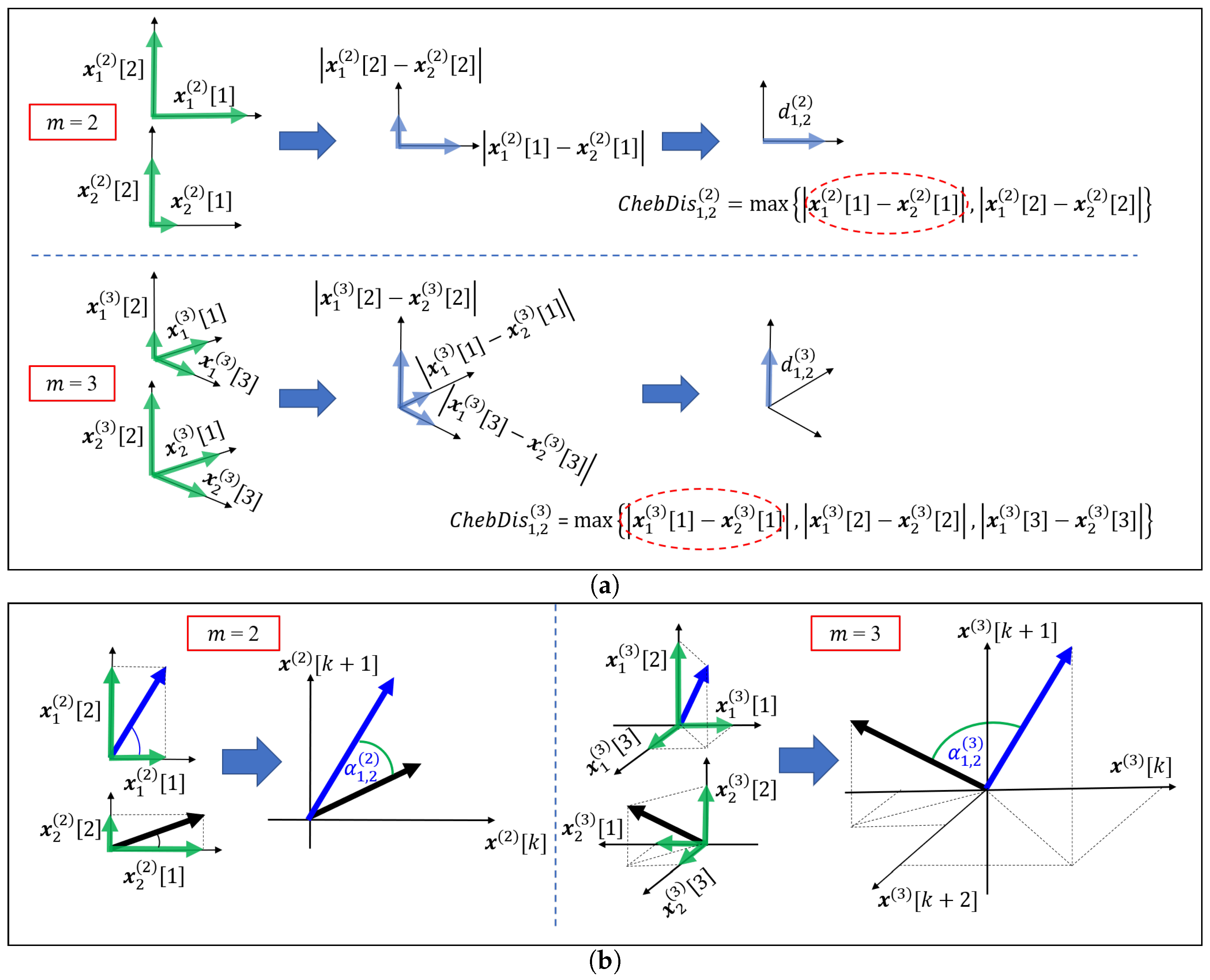
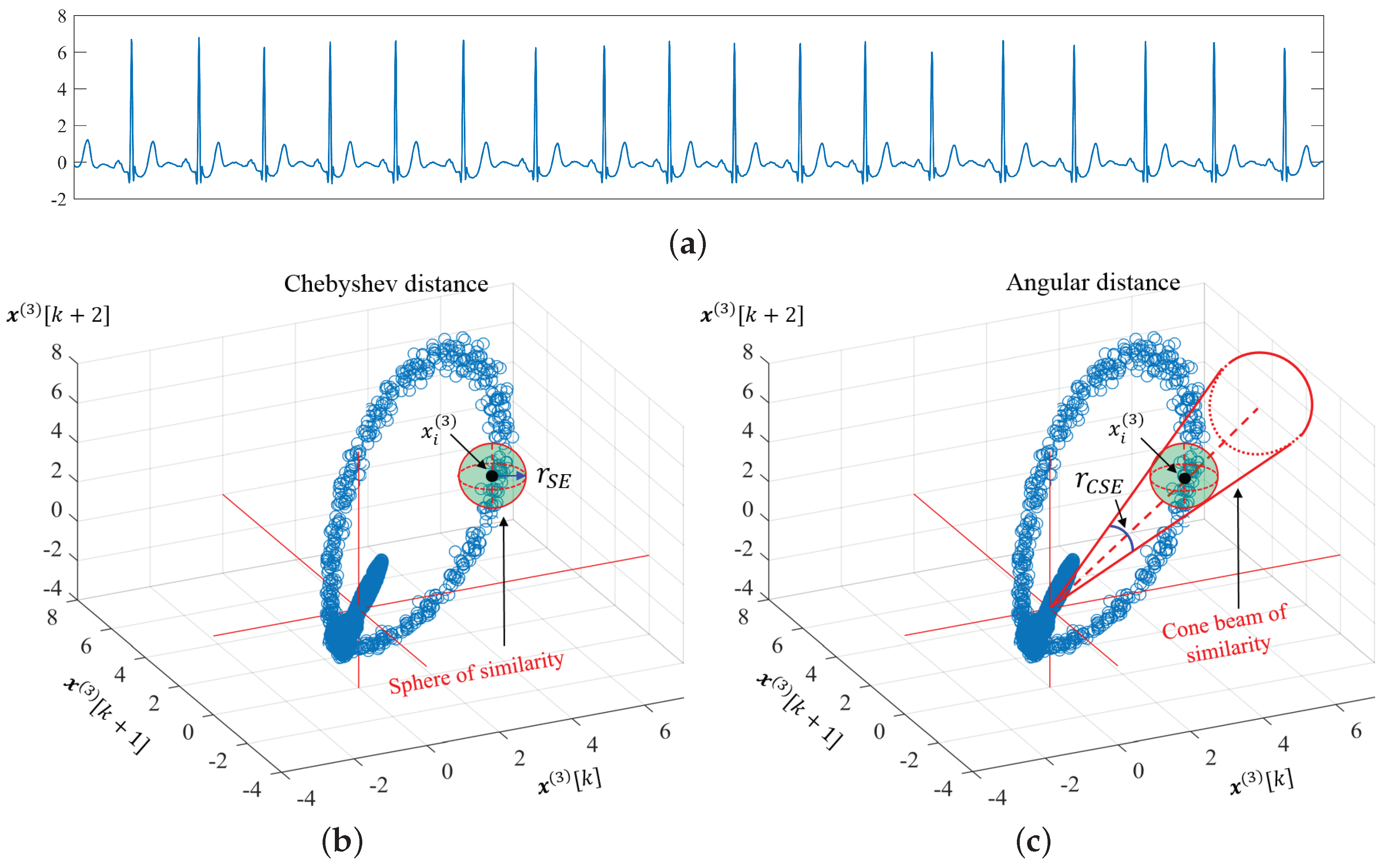
3.1. Angular Distance

The Chebyshev distance used in the SE is obtained from the maximum amplitude difference among elements of the two embedding vectors (for a given m); however, this amplitude-based distance is sensitive to spikes or erratic peaks in data. In the sense of structural similarity, it is reasonable to consider similar patterns as spans of a prototype vector, or, alternatively, any embedding vectors that are scaled by multiplying gains (within a given small tolerance). With this rationale, we show that the angular distance metric ( A n g D i s ), which rests upon of the angle between two embedding vectors, is an appropriate choice for the determination of the similar patterns in a noisy time series. The major advantage of the angular distance is its low sensitivity to any changes in vector norms as long as the angle between the considered vectors is maintained, thus providing the desired amplitude-independent-based distance.

3.2. Properties of Angular Distance

It is important to mention that the angular distance belongs to the family of cosine distances ( C o s D i s ) which are derived from the cosine similarity ( C o s S i m ) metric. Cosine similarity is defined as an inner product of two vectors divided by the product of their norms, giving a range from 1 to 1. To produce a distance metric allowing for only positive values, the cosine distance is simply modified by subtracting its value from 1, to yield a range from 0 to 2. However, the cosine similarity and the cosine distance are not proper distance metrics, as they violate the triangle inequality property of a metric in normed vector spaces [25,26]. Prior to illustrating this phenomenon, the properties of any valid distance metrics are summarized in the following. Let a , b , c be arbitrary vectors in a subspace of R m and D i s ( a , b ) a distance between the vector a and vector b . The properties of a valid distance are: (i) non-negativity ( D i s ( a , b ) 0 ) ; (ii) identity of indiscernibles ( D i s ( a , b ) = 0 only if a = b ); (iii) symmetry ( D i s ( a , b ) = D i s ( b , a ) ); and (iv) triangle inequality ( D i s ( a , b ) D i s ( a , c ) + D i s ( c , b ) ) [23,24]. Even though the cosine distance is not a proper distance, it has been used in some applications, such as face recognition [27], speech processing [28] and text mining [29]. The angular distance is defined as a normalized angle between two vectors and is calculated as c o s 1 ( C o s S i m ) divided by π , so that the boundary values of the angular distance range from 0 to 1. This means that two vectors are similar when A n g D i s approaches 1 and dissimilar when A n g D i s approaches 0. The properties of the angular distance now do obey the axioms of a proper distance metric, including the triangle inequality [30].
For a given embedding vector m, the cosine similarity, C o s S i m i , j ( m ) , cosine distance, C o s D i s i , j ( m ) , actual angle, α i , j ( m ) , and angular distance, A n g D i s i , j ( m ) , of any two embedding vectors x i ( m ) and x j ( m ) where i j are defined as
C o s S i m i , j ( m ) = x i ( m ) · x j ( m ) | x i ( m ) | | x j ( m ) | ,
C o s D i s i , j ( m ) = 1 C o s S i m i , j ( m ) ,
α i , j ( m ) = c o s 1 ( C o s S i m i , j ( m ) ) ,
A n g D i s i , j ( m ) = α i , j ( m ) π .
The geometric interpretation of A n g D i s and C h e v D i s in the Euclidean space is given in Figure 1, and the geometric interpretation of similar patterns obtained using the Chebyshev distance and the angular distance in Figure 2.
Despite its obvious amplitude independence, the angular distance is sensitive to any offsets in a time series, including baseline wander, generally present in real world signals. To eliminate the influence of offsets, the centered cosine similarity version (or so-called Pearson correlation [31,32]), including its corresponding distance called “distance correlation”, was introduced in [33]. Both methods effectively reduce the influence of the offset by centering the input vectors based on their own vector means. In addition, such methods are usually applied to two vectors containing a number of samples big enough to faithfully represent their intrinsic distributions (i.e., high dimensional vectors), so that their vector means are a good proxy to the global means of the population. However, in practice the reconstructed embedding vectors are of low dimensions, e.g., m = 2 or m = 3 [2], so that centering such embedding vectors by their local means would disrupt the accuracy of their global correlation estimate and could lead to bias when examining similar patterns. To resolve this issue, while preserving its amplitude range (unnormalized amplitude), we propose a simple (optional) pre-processing to remove such global offset by using a zero-median method [34]. We opt for the zero-median rather than the zero-mean approach because of its robustness to outliers and spikes, erratic amplitudes to which the zero-mean approach is sensitive. With such pre-processing, the angular distance is made robust to baseline wander.

3.3. Cosine Similarity Entropy and Multiscale Cosine Similarity Entropy

The robust entropy algorithm proposed in this study is referred to as the “Cosine Similarity Entropy” (CSE), whereby, for consistent entropy estimation within a general framework of Algorithm 1, the Chebyshev distance is replaced with the angular distance and Shannon entropy is employed instead of the standard conditional probability. The Shannon entropy is mathematically described as
H ( x ) = i = 1 n p ( x i ) log b p ( x i ) ,
where p ( x i ) is the probability mass function of random variables x i = x 1 , x 2 , , x N .
For a case of 1-bit data length ( n = 2 ) with a given logarithm base b = 2, Shannon entropy can be written as
H ( x ) = ( p ( x 1 ) log 2 p ( x 1 ) + p ( x 2 ) log 2 p ( x 2 ) ,
where p ( x 1 ) is the probability mass function of the random variables x 1 = 0 and p ( x 2 ) is the probability mass function of the random variables x 2 = 1
Recall that p ( x 1 ) + p ( x 2 ) = 1 , so the Equation (9) can be re-written as
H ( x ) = [ p ( x 1 ) log 2 p ( x 1 ) + p ( 1 x 1 ) log 2 p ( 1 x 1 ) ] .
Notice that unlike for the standard SE, the undefined entropy values now only occur when p ( x i ) = 0 , meaning that none of the similar patterns is found for a given tolerance level (which is unlikely to happen). When the 1-bit data length has a uniformly distributed probability function, p ( x 1 ) = p ( x 2 ) = 0.5 , the unique maximum entropy calculated from Equation (10) is 1, and thus H ( x ) ranges from 0 to 1.
In the proposed CSE algorithm, the computational steps in the SE approach, given in Algorithm 1, are replicated with three modifications: (i) in the first step of the SE, we provide optional pre-processing for removing the offset in a time series; (ii) in the third step of the SE, angular distance is used instead of the Chebyshev distance; and (iii) in the last step of the SE, we estimate the entropy based on Equation (10), by substituting the global probability of occurrences of similar patterns B ( m ) ( r C S E ) and its complementary probability ( 1 B ( m ) ( r C S E ) ) for the terms p ( x 1 ) and p ( x 2 ) . The steps of the CSE approach are summarized in Algorithm 3.
Algorithm 3. Cosine Similarity Entropy
For a time series { x i } i = 1 N with given embedding dimension (m), tolerance ( r C S E ) and time lag ( τ ):
  • (Optional pre-processing) Remove the offset and generate a zero median series { g i } i = 1 N as
    g i = x i m e d i a n ( { x i } i = 1 N ) .
  • Construct the embedding vectors, x i ( m ) from { x i } i = 1 N or from { g i } i = 1 N using
    x i ( m ) = [ x i , x i + τ , , x ( i + ( m 1 ) τ ) ]   or   x i ( m ) = [ g i , g i + τ , , g ( i + ( m 1 ) τ ) ] .
  • Compute angular distance for all pairwise embedding vectors as
    A n g D i s i , j ( m ) = 1 π c o s 1 ( x i ( m ) · x j ( m ) | x i ( m ) | | x j ( m ) | ) , i j .
  • Obtain the number of similar patterns P i ( m ) ( r C S E ) when a criterion A n g D i s i , j ( m ) r C S E is fulfilled.
  • Compute the local probability of occurrences of similar patterns, B i ( m ) ( r C S E ) , as
    B i ( m ) ( r C S E ) = 1 ( N n 1 ) P i ( m ) ( r C S E ) .
  • Compute the global probability of occurrences of similar patterns, B ( m ) ( r C S E ) , from
    B ( m ) ( r C S E ) = 1 N n i = 1 N m B i ( m ) ( r C S E ) .
  • Cosine similarity entropy is now estimated from
    C S E ( m , τ , r C S E , N ) = [ B ( m ) ( r C S E ) log 2 B ( m ) ( r C S E ) + ( 1 B ( m ) ( r C S E ) ) log 2 ( 1 B ( m ) ( r C S E ) ] .
For the multiscale cosine similarity entropy (MCSE) algorithm, only the coarse graining process is required prior to proceeding with other steps in the CSE. For a given scale factor ϵ , the coarse-grained scale produced from Equation (1) is substituted for x i i = 1 N to serve as an input to the CSE algorithm, and the estimation of the multiscale cosine similarity entropy is given by
M C S E ( m , τ , r C S E , N , ϵ ) = [ B ( ϵ ) ( m ) ( r C S E ) log 2 B ( ϵ ) ( m ) ( r C S E ) + ( 1 B ( ϵ ) ( m ) ( r C S E ) ) log 2 ( 1 B ( ϵ ) ( m ) ( r C S E ) ] ,
where B ( ϵ ) ( m ) ( r C S E ) and B ( ϵ ) ( m + 1 ) ( r C S E ) are, respectively, the global probabilities of occurrences of similar patterns for a given m and ( m + 1 ) .
Note that, in the SE and FE algorithms, C h e b D i s can be obtained for any two embedding vectors with a minimal m = 1 , since the distance is based on the operation on individual element of two vectors, while in the CSE, A n g D i s can be obtained for any two embedding vectors with a minimal m = 2 , since vectors with a single dimension are always aligned to their single basis vector, which is considered a trivial angular distance, so that A n g D i s in valid only when applied to vectors with m 2 (see Equations (4)–(7) and Figure 1); this is practically perfectly valid.

4. Selection of Parameters
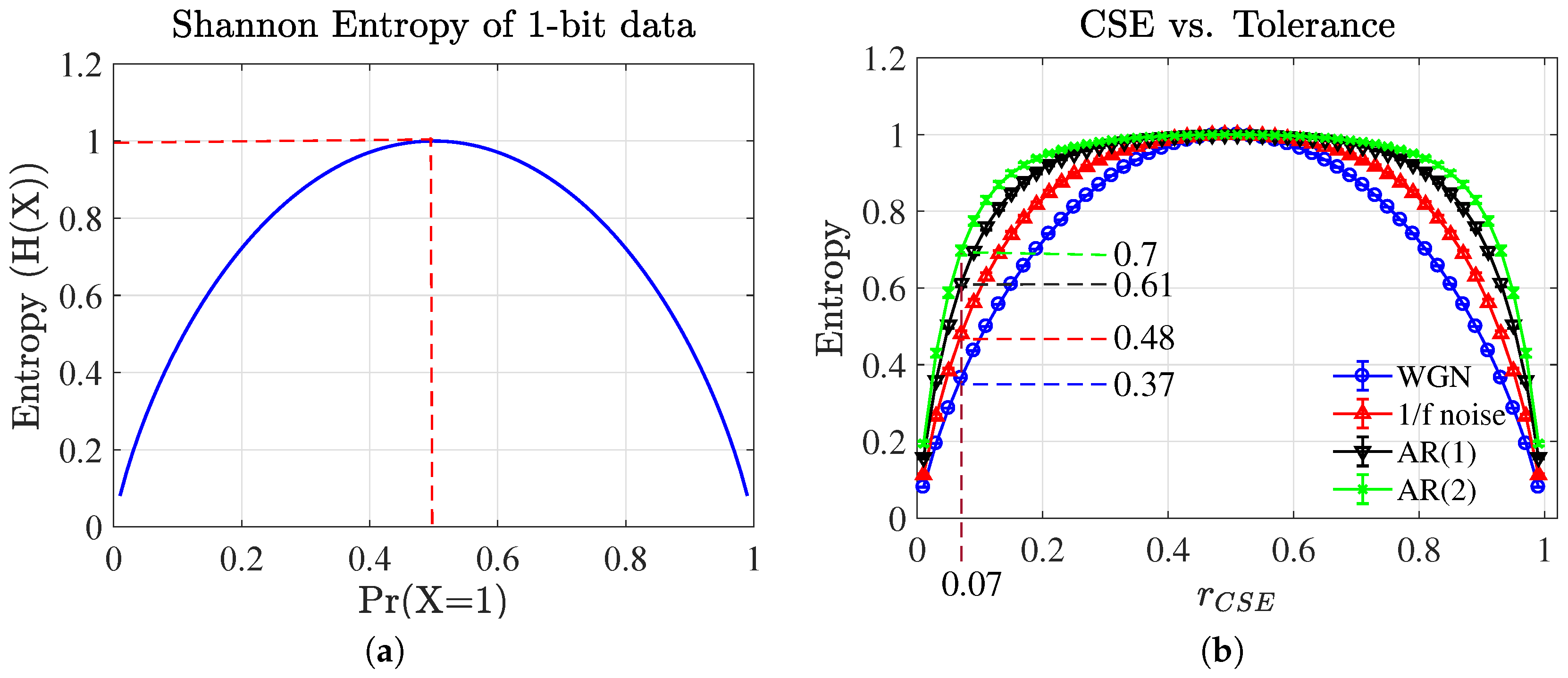
Selection and robustness of the parameter values of the proposed CSE approach is next demonstrated over several benchmark scenarios.

4.1. Selection of the Tolerance ( r C S E ) for CSE

In the SE and the FE approaches, the tolerance parameter is defined as a product of a given ratio value (r) and the standard deviation (SD) of a considered time series, that is, r S E = r F E = r × S D . The recommended tolerance level, r S E , for the SE, is between 0.1 and 0.25 [7,35]. The recommended tolerance level, r F E , for the FE is between 0.1 and 0.3 [11]. In our proposed CSE and MCSE algorithms, we examined how entropy changes as a function of r C S E on four synthesized signals: (i) White Gaussian Noise (WGN); (ii) 1 / f noise; (iii) the first order autoregressive model (AR(1)) generated from x ( t ) = 0.9 x ( t 1 ) + ε ( t ) and (iv) the second order autoregressive model (AR(2)) generated from x ( t ) = 0.85 x ( t 1 ) + 0.1 x ( t 2 ) + ε ( t ) , where ε ( t ) N ( 0 , 1 ) . We generated 20 independent realizations with 10,000 samples for each synthetic signal with the recommended m = 2 [2], τ = 1 [36], and varied r C S E from 0.01 to 0.99 with an incremental step of 0.02 (as the boundary values of the angular distance ranges from 0 to 1). Since Shannon entropy is employed in the proposed CSE algorithm, it is anticipated that the outcomes of the CSE versus r C S E are analogous to the properties of Shannon entropy versus probability of a selected event, P r ( X = 1 ) , when using 1-bit data, as shown in Figure 3a. Figure 3b illustrates the results of the CSE plotted as mean entropies with their SD against r C S E . Observe a rise of mean entropies in all the four CSE curves from low to high entropy with an increase in r C S E from 0.01 to 0.49, and a decrease in mean entropies in all the four curves with an increase of r C S E from 0.51 to 0.99. This means that, as anticipated, the characteristics of the CSE resemble the characteristics of the Shannon entropy, whereby the unique maximum entropy occurs at r C S E = 0.5 . We can thus approximately define an optimal range of the r C S E for which the mean entropies of the four synthetic signals are (visually and statistically) discernable to between 0.05 and 0.2 (the range of r C S E between 0.5 and 1 can also be used, but we considered the lower region of r C S E due to the fact that the smaller the tolerance the greater the similarity). For a comparison between the mean entropies among the four synthetic signals, we empirically selected r C S E = 0.07 , for which the corresponding mean entropies of the WGN, 1 / f noise, AR(1) and AR(2) were, respectively, 0.37, 0.48, 0.61 and 0.7.

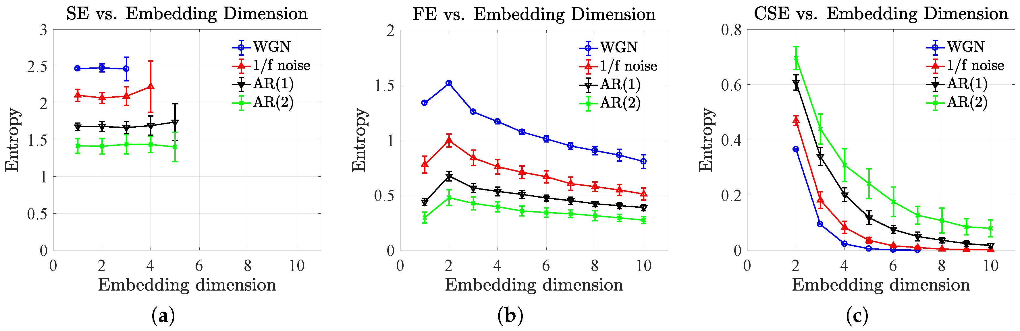
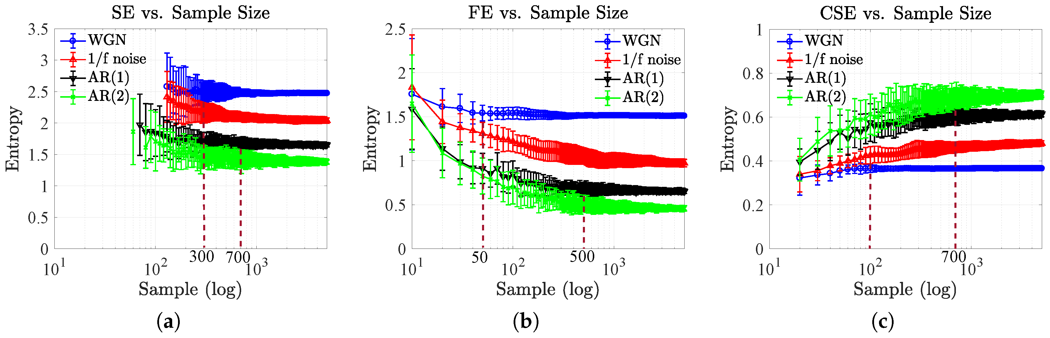
4.2. Effect of Sample Size and Embedding Dimension

The sample size, N, and embedding dimension, m, are important parameters which affect the outcomes of the SE and FE approaches (we do not consider varying the time lag, τ , parameter because this is analogous to a number of samples used in downsampling. Hence, we fix τ = 1 [36] for the structural preservation of the original data). In practical applications, it is acceptable to select a small embedding dimension such as m = 2 [2,11,37,38] for both approaches, while the rule of thumb for an appropriate N is as low as 10 m 30 m for the SE [7,35]; however, for the FE, the data length N can be selected to be as little as 50 samples [11]. We next tested the performances of the three entropy approaches (SE, FE and CSE) as a function of: (1) embedding dimension and (2) sample size. In the first test, we generated 30 realizations for each of the four synthetic signals; WGN, 1 / f noise, AR(1) and AR(2), as mentioned in Section 4.1, with the selection of N = 1000 , τ = 1 , r S E = r F E = 0.15 , r C S E = 0.07 and η = 2 (an order of the Gaussian membership function used in the FE [11]), while varying m from 1 to 10 (for the CSE, m was varied from 2 to 10 as mentioned in Section 3). In the second test, we generated 30 independent realizations for each of the four synthetic signals with the values of m = 2 , τ = 1 , r S E = r F E = 0.15 , r C S E = 0.07 and η = 2 , while varying N with three different step sizes: (i) for the sample sizes from 10 to 1000, the incremental step was 10 samples (N = 10:10:1000); (ii) for the sample sizes from 1020 to 2000, the incremental step was 20 samples (N = 1020:20:2000); and (iii) for the sample sizes from 2050 to 5000, the incremental step was 50 samples (N = 2050:50:5000). A performance comparison in terms of computational time used for the three entropy algorithms with different sample sizes of data is also examined and described in Appendix C.
Figure 4 shows the results of the first test (varied m) plotted as mean entropies with their SD against m. Figure 4a depicts the results of the SE where the mean entropies behaved consistently over different ranges of m for each synthetic signal: (i) WGN: m = [ 1 , 2 , 3 ] ; (ii) 1 / f noise: m = [ 1 , 2 , 3 , 4 ] ; (iii) AR(1) and AR(2): m = [ 1 , 2 , , 5 ] . However, for any m outside the ranges mentioned, the SE resulted in undefined entropy. Figure 4b illustrates the results of the FE in which the mean entropies of all synthetic signals showed a slow decline with an increase in m (from 2 to 10), and the mean entropies peaked at m = 2 . Figure 4c shows the results of the CSE in which the mean entropies decreased with an increase in m, and when m 6 , the mean entropies of the WGN and 1 / f noise approached zero. The CSE showed a characteristic loss in entropy values at large embedding dimensions that corresponds to the assumption in [3,39], which states that, when increasing m, the trajectory of the embedding vectors reconstructed from an observed time series become more and more predictable (for m the trajectory would become deterministic). In terms of predictability, this implies that for the CSE, the larger the embedding dimension, the lower the complexity (lower entropy), unlike the FE method that produced relatively stable mean entropies over all scale factors (including the SE method but with the valid mean entopies at the low embedding dimensions).
Remark 1.
From Figure 4, the CSE yields valid entropy values over a broad range of embedding dimensions ( m = [ 2 , 3 , , 10 ] ), while the SE gives valid entropy values only for a small m = [ 1 , 2 , 3 ] .
Figure 5 shows the results of the second test (varied N) plotted as mean entropies with their SD against N. Figure 5a depicts the results of the SE approach in which the entropy values of the WGN and 1 / f noise were valid for N 130 , for the AR(1), entropy was valid for N 70 , and, for the AR(2), entropy was valid for N 60 . By visually selecting any N at which the SD of the two mean entropies were non-overlapped, the separation of mean entropies between the WGN and the 1 / f noise was significant when N 300 , and for the AR(1) and the AR(2) the separation was achieved when N 700 . Figure 5b illustrates the results of the FE in which the entropy of all synthetic signals was valid over the whole range of the sample sizes. The separation of mean entropies between the WGN and the 1 / f noise was discernible when N 50 , and, for the AR(1) and the AR(2), the separation of mean entropies was pronounced when N 500 . Figure 5c shows the results of the CSE approach in which the entropy of all synthetic signals was valid even when the numbers of samples was as low as N = 20 . The separation of mean entropies between the WGN and the 1 / f noise was observed when N 100 , while for the AR(1) and AR(2), the separation of mean entropies was pronounced when N 700 . Notice that all approaches gave stable entropy values for the large sample sizes N 1000 , and, at N = 1000 , the CSE yielded the smallest SD, compared to other approaches as shown in Table 1.
Remark 2.
From Figure 5, for the separation of mean entropies between WGN and 1 / f noise, the CSE requires a smaller sample size ( N = 100 ) than the SE ( N = 300 ). The CSE also yields the smallest SD compared to other approaches; in other words, the CSE produces the smallest variation of entropy values.

5. A Comparison of Complexity Profiles Using MSE, MFE and MCSE

After having established the basic properties of the proposed CSE approach, we now evaluate the usefulness of its multiscale version, the multiscale CSE (MCSE), for the quantification of the structural complexity over the coarse-grained scales.

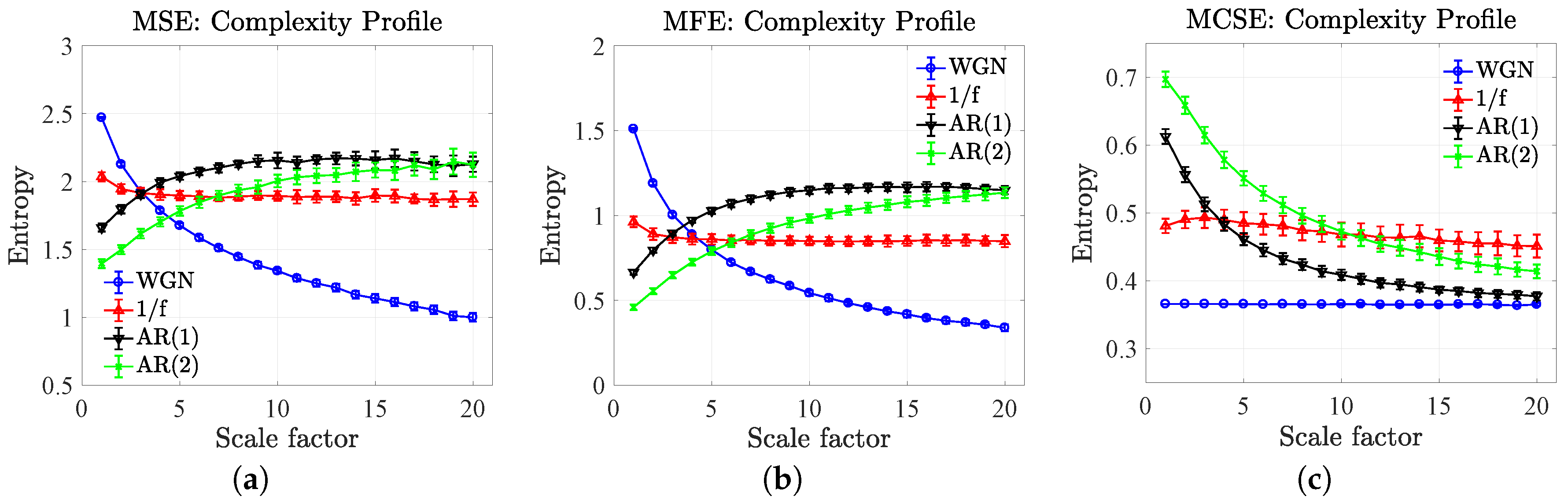
5.1. Complexity Profiles of Synthetic Noises

To examine the behaviors of the multiscale versions-MSE, MFE and MCSE-over the coarse-grained scales (complexity profiles [20]), we generated 20 independent realizations of 10,000 samples for each of the four synthetic signals; WGN, 1 / f noise, AR(1) and AR(2), as described in Section 4.1. For the three multiscale entropy approaches, we selected m = 2 [19], τ = 1 , r S E = r F E = 0.15 , r C S E = 0.07 , η = 2 and the scale factor, ϵ , from 1 to 20. Figure 6 illustrates the results of the three approaches plotted as mean entropies with their SD against the scale factors. Figure 6a depicts the results of the MSE from which distinctive profiles of the entropy curves can be observed. At ϵ = 1 , the order of the mean entropies from high to low corresponded to the WGN, 1 / f noise, AR(1) and AR(2), while, at a large scale, ϵ = 20 , both the AR(1) and AR(2) yielded the highest mean entropies, and the lower mean entropies were for the 1 / f noise followed by the WGN. The distinctive behaviors for the synthetic signals can be described as follows: (i) for the WGN, the entropy curve decreased as the scale increased; i.e., at ϵ = 1, the mean entropy was 2.5, and at ϵ = 20 , the mean entropy fell to 1.0; (ii) for the 1 / f noise, the entropy curve was relatively consistent over all scale factors (mean entropies varied between 1.87 and 2.04); (iii) for the AR(1) and AR(2), the entropy curves gradually ascended as the scale increased; i.e., at 1 ϵ 17 , the entropy curve of the AR(1) was above the entropy curve of the AR(2) while at ϵ 18 , the entropy curves of both the AR(1) and AR(2) converged and then overlapped at the mean entropy values of 2.12. Figure 6b shows the results of the MFE approach in which all the entropy curves were similar to the corresponding entropy curves of the MSE. The only difference was that the MFE produced lower mean entropies than the MSE. Figure 6c illustrates the results of the MCSE from which distinctive complexity profiles can be observed. At ϵ = 1 , the order of high to low mean entropies was the AR(2), AR(1), 1 / f noise and WGN, while, at ϵ = 20 , the order of high to low mean entropies was the 1 / f noise, AR(2), AR(1) and WGN, that is, the correct order of structural complexity. This can be explained as follows: (i) for the WGN, the mean entropy value of 0.37 was consistent over the whole range of the scale factors; (ii) for the 1 / f noise, the entropy curve either slowly decreased or was almost consistent, with small variation of mean entropies (between 0.45 and 0.49), and, as desired, the mean entropies of the 1 / f noise were higher than those of the WGN over all the scale factors; (iii) for the AR(1) and AR(2), the entropy curves gradually decayed as the scale factor increased, and, as desired, the entropy curves of the AR(1) were lower than those of the AR(2) for the whole range of the scale factors; i.e., at ϵ = 1 , mean entropies of the AR(1) and AR(2) had the values of 0.61 and 0.7, while at ϵ = 20 , the mean entropies the AR(1) and the AR(2) were 0.38 and 0.41.
Remark 3.
From Figure 6, at large scale factors, the MCSE provides a well defined separation of mean entropies among all the synthetic signals, WGN, 1 / f noise, AR(1) and AR(2), while the MSE and MFE only yield a good separation of mean entropies between the WGN and the 1 / f noise. In addition, unlike MSE and MFE, for the proposed MCSE, the complexity of the 1 / f noise was higher than that of the WGN for the whole range of the scale factors, thus completing the physical meaningless of the MFE and MSE.

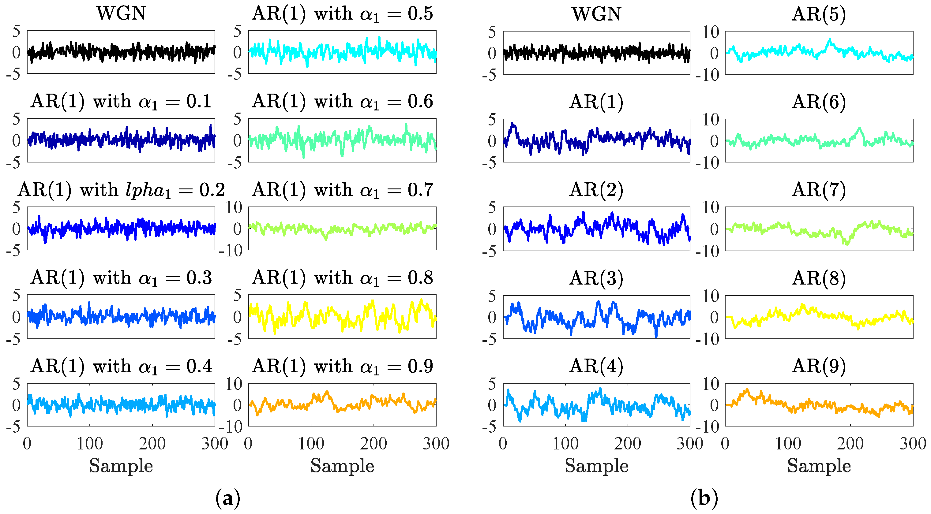
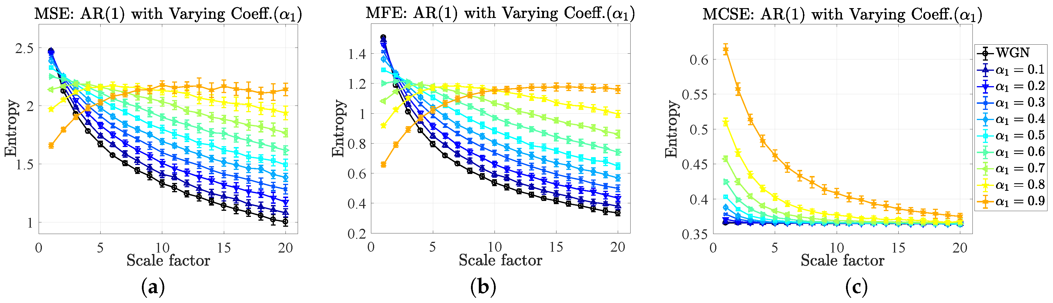
5.2. Complexity Profiles of Autoregressive Models

We next examined the complexity profiles of an ensemble of autoregressive processes (AR) over the coarse-grained scales, through the MSE, MFE and MCSE. To this end, we generated two groups of AR processes: (i) AR(1)s processes with nine different correlation coefficients ( α 1 , where α 1 = [ 0.1 , 0.2 , , 0.8 , 0.9 ] ) and (ii) AR(p) processes of nine different orders (p, where p = [ 1 , 2 , , 8 , 9 ] ) with the pre-defined correlation coefficients (more details of the processing for both groups of the AR are described in Appendix A). We generated 20 independent realizations of 10,000 samples for the WGN, which were also used as the driving noise for all nine of the AR(1)s and for all of the nine orders of the AR(p) processes. For the three multiscale entropy approaches, we selected m = 2 , τ = 1 , r S E = r F E = 0.15 , r C S E = 0.07 , η = 2 and ϵ from 1 to 20.
Remark 4.
Our hypothesis was that a consistent complexity estimator should give the same quantification of complexity order for all nine AR(1) processes over a range of scale factors, independent of the correlation coefficient, as all these AR(1) processes have only a single degree of freedom. Similarly, the complexity of the AR(p) processes, p = [ 1 , 2 , , 9 ] , should increase with the order p, independent of their correlation profile.
Figure 7 illustrates the results of the three approaches applied to the first group of the synthetic AR processes. The results are plotted as mean entropies with their SD against the scale factors. Figure 7a depicts the results of the MSE; at ϵ = 1 , the WGN yielded the highest mean entropy, and the lower mean entropies were ranked in a descending order corresponding to the low to high correlation coefficients of the AR(1) (i.e., α 1 = [ 0.1 , 0.2 , , 0.8 , 0.9 ] ). At ϵ = 20 , the mean entropies were ranked in a descending order corresponding to the high to low correlation coefficients of the AR(1) (i.e., α 1 = [ 0.9 , 0.8 , , 0.2 , 0.1 ] ), while the lowest mean entropy was that of the WGN. Figure 7b shows the results of the MFE where all the entropy curves were similar to the corresponding entropy curves of the MSE. The only difference was that the MFE produced lower mean entropies than those of the MSE. Figure 7c illustrates the results of the MCSE from which distinctive profiles of the entropy curves can be observed. At ϵ = 1 , the mean entropies were ranked in a descending order corresponding to the high to low correlation coefficients of the AR(1) (i.e., α 1 = [ 0.9 , 0.8 , , 0.2 , 0.1 ] ), while the lowest mean entropy belonged to the WGN, which was constantly 0.37 for the whole range of the scale factors. At a large scale, ϵ = 20 , the mean entropies were ranked in a descending order corresponding to the decreasing correlation coefficients of the AR(1). Notice that, as described, all the entropy curves asymptotically converged, indicating that all the AR(1) processes have the same structural complexity, that is, one degree of freedom.
Remark 5.
From Figure 7, for an ensemble of AR(1) processes with a varying correlation coefficients, the MCSE, unlike the other methods considered, provided robust, accurate and physically meaningful quantification of complexity of the system. In other words, only the MCSE was able to assess the correct complexity of the underlying signal-generation system, the AR(1).
Figure 8 illustrates the results of the three approaches applied to the second group of synthetic AR processes. The results are plotted as mean entropies with their SD against the scale factors. Figure 8a depicts the results of the MSE; at ϵ = 1 , WGN yielded the highest mean entropy, and remaining mean entropies were ranked in a descending order corresponding to the low to high orders of the AR(p) processes (i.e., p = [ 1 , 2 , , 9 ] ), while, at ϵ = 20 , the mean entropies were ranked in a descending order corresponding to the order AR(p) processes as AR(3), AR(4), both the AR(2) and AR(5) (overlapped), AR(6), AR(1), AR(7), AR(8), AR(9), and the lowest mean entropy belonged to WGN. Figure 8b shows the results of the MFE in which all the entropy curves were similar to the entropy curves of the MSE. The two differences were that: (i) the MFE produced lower mean entropies than those of the MSE; and (ii) at ϵ = 20 , the mean entropies of the AR(2) were higher than that of the AR(5) (not overlapped as the result of the MSE). Figure 8c illustrates the results of the MCSE, with the correct distinctive profiles of the entropy curves observed. At ϵ = 1 , the mean entropies were ranked in a descending order corresponding to the high to low orders of the AR(p) processes (i.e., p = [ 9 , 8 , , 1 ] ), and the lowest mean entropy was that of the WGN (no structure), with a constant value of 0.37 over the whole range of the scale factors. At a large scale, ϵ = 20 , the mean entropies of the AR(p)s were ranked in a descending order corresponding to the order of the AR(p)s as at ϵ = 1 . Notice that all the entropy curves exhibited a slight decrease in their mean entropies with an increase in the scale factor.
Remark 6.
From Figure 8, only the proposed MCSE complexity estimate was able to correctly distinguish between the structural complexities of the signal-generation systems, which ranged in an increasing order, from one degree of freedom (AR(1)) to nine degrees of freedom (AR(9)). Importantly, this was achieved independent of the correlation profile of the so generated signals.

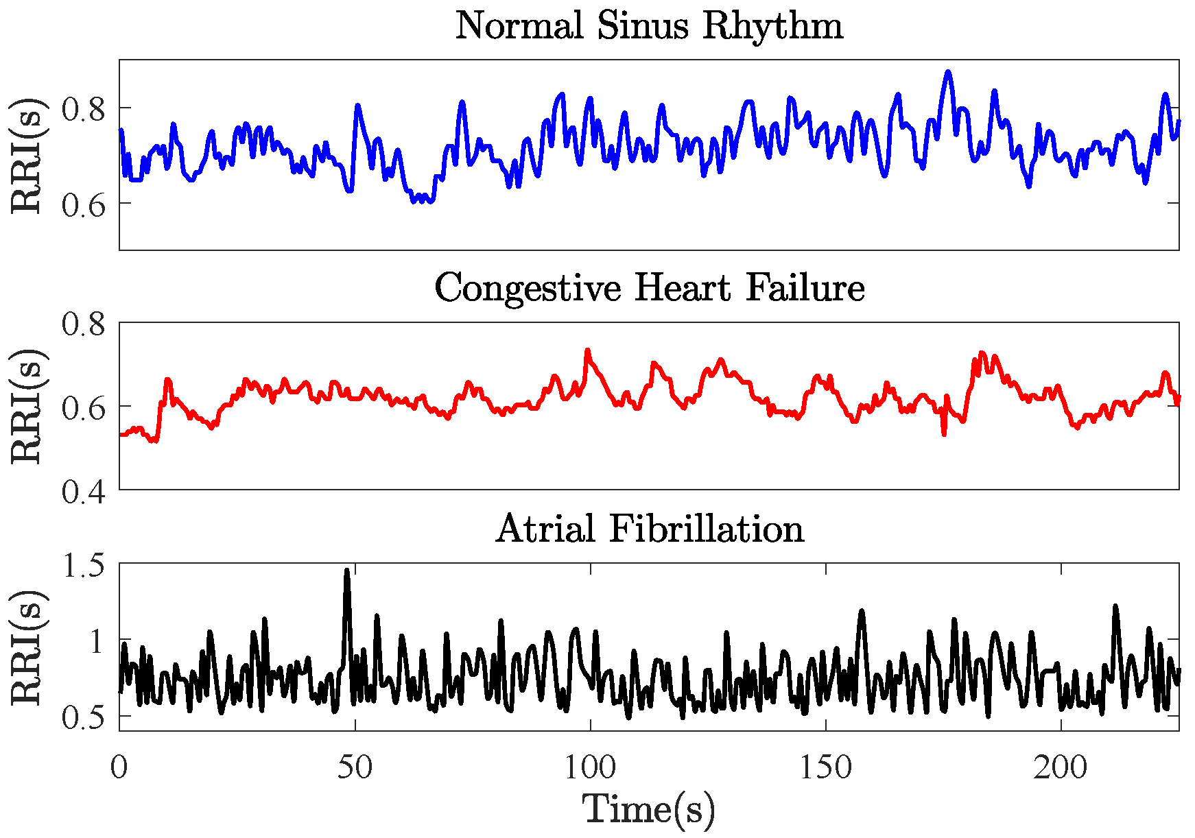
5.3. Complexity Profiles of Heart Rate Variability

We next examined the entropy behavior of heart rate variability (HRV) over the coarse-grained scales through the MSE, MFE and MCSE. Three cardiovascular pathologies of one-hour RR intervals: (i) Normal Sinus Rhythm (NSR, 18 subjects); (ii) Congestive Heart Failure (CHF, 20 subjects); and (iii) Atrial Fibrillation (AF, 20 subjects) were obtained from the Physionet database (for more details, see Appendix B). We estimated the HRV time series of the three cardiac conditions by re-sampling the obtained RR intervals at the frequency of 8 Hz using the shape-preserving piecewise cubic interpolation. The HRVs were segmented into trials of 10-min length. For the three multiscale approaches, we selected m = 2 , τ = 1 , r S E = r F E = 0.15 , r C S E = 0.07 , η = 2 and varied ϵ from 1 to 20.
Figure 9 illustrates the results of the three approaches plotted as mean entropies with their standard errors (se) against the scale factors. Figure 9a depicts the results of the MSE; at ϵ = 1 , AF and NSR yielded the highest mean entropies (the mean entropy of the AF (0.36) was slightly higher than the mean entropy of the NSR (0.31)), and the CHF yielded the lowest mean entropy (mean entropy was 0.2). At ϵ = 20 , the order of the mean entropies from high to low was the NSR, AF and CHF. Figure 9b shows the results of the MFE where all the entropy curves were similar to the entropy curves of the MSE. The only two differences were: (i) the MFE produced lower mean entropies than the MSE; (ii) at ϵ = 1 , the highest mean entropy was to the AF (0.17), followed by the mean entropies of both the CHF and NSR (overlapped at 0.08). Figure 9c illustrates the results of the MCSE; at ϵ = 1 , the order of the mean entropies from high to low was the NSR, CHF and AF (the mean entropy of the CHF (0.89) was slightly higher than the mean entropy of the AF (0.88)), while, at the ϵ = 20 , the order of the mean entropies from high to low was the CHF, NSR and AF.

6. Discussion and Conclusions

We have introduced the Cosine Similarity Entropy (CSE) and the Multiscale Cosine Similarity Entropy (MCSE) algorithms to robustly quantify the structural complexity of real-world data. This has been achieved based on the similarity of embedding vectors, evaluated through the angular distance, the Shannon entropy and the coarse-grained scale. We have examined the properties of the CSE by varying the tolerance level and have found the optimal range for the tolerance to be between 0.05–0.2. The effects of the parameters, including the embedding dimension and the sample size, on the three approaches, the Sample Entropy (SE), Fuzzy Entropy (FE) and CSE, have been initially evaluated over the four synthetic signals, the WGN, 1 / f noise, and an ensemble of AR(1) and AR(2) linear stochastic processes. The appropriate selection of m and N for the three approaches is summarized in Table 2 (the low embedding dimension, m = 2 [19], is recommended for the multiscale versions; MSE, MFE and MCSE, due to a decrease in the number of samples with an increase in the scale factor). The advantage of the CSE over the SE is shown to be that the CSE requires a small sample size for the separation of mean entropies between WGN and 1 / f noise (the CSE requires 100 samples while the SE requires 300 samples), a critical issue in real-world recordings. Events though the FE require the minimum sample size compared to the sample sizes required in the SE and CSE, and the CSE has been outperformed the SE and FE in terms of variations (SD) of mean entropies, as shown in Table 1.
The proposed CSE algorithm has been demonstrated to quantify degrees of self-correlation-based complexity in a time series rather than to quantify degrees of uncertainty-based complexity as in the SE and FE algorithms, and to be signal amplitude independent—a key obstacle for current nonparametric entropy measures. We have also determined how the entropy values of the four benchmark synthetic signals, WGN, 1 / f noise, AR(1) and AR(2), behave over the coarse-grained scale, so-called complexity profiles, through the corresponding multiscale versions, MSE, MFE and MCSE. The results of the MSE and MFE at the first scale factor have revealed that the degrees of the structural complexity (uncertainty-based) from high to low correspond to the WGN, 1 / f noise, AR(1) and AR(2), whereas the MCSE provides entropy values sorted based on the degrees of the structural complexity (self-correlation-based), from high to low, as AR(2), AR(1), 1 / f noise and WGN. In terms of self-correlation, as an uncorrelated signal, WGN has no structure, the 1 / f noise is a long-term correlated signal and hence with maximum structure, and the AR(1) and AR(2) processes exhibit different degrees of short-term correlation, whereby the AR(2) can be more correlated than the AR(1) owing to its higher order (more degrees of freedom or more correlated terms). Therefore, at a small scale factor (short-term), the degrees of the self-correlation-based complexity from high to low correspond to the AR(2), AR(1), 1 / f noise and WGN, while, at a large scale factor (long-term), the degrees of the self-correlation-based complexity ordered from high to low correspond to the correct order, 1 / f noise, AR(2), AR(1), and WGN. We have found that only the results from the MCSE have been able to correctly reveal this short- to long-term structural complexity order and to give physically meaningful entropy and complexity estimates. The results of the MCSE have also shown that the mean entropies of WGN have yielded the lowest complexity and were consistent over the whole range of the scale factors, meaning that the WGN has no correlation in the short- or long-term and can thus be used as a “reference complexity” (no structure in an uncorrelated signal).
We have also tested the three approaches over nine varying correlation coefficients of the AR(1) process, and nine increasing orders of the AR(p) process. We have hypothesized that the low to high degrees of complexity are in a direct relationship with the small to large values of the correlation coefficients of the AR(1), and the increasing orders of the AR(p) (degrees of freedom), and have found that the results of the three multiscale entropy estimates quantify relationships with these AR processes as follows:
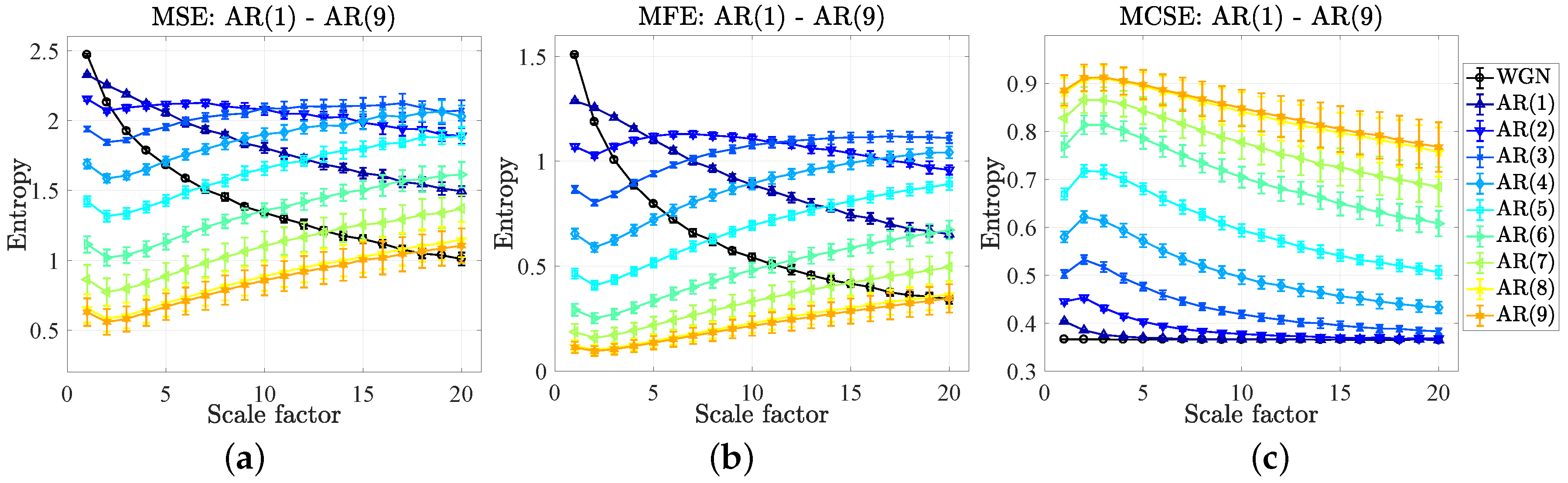
  • The results of the MSE and MFE have unveiled that the high to low mean entropies (complexity) were in agreement with the high to low values of the correlation coefficients of the AR(1) only at the large scale factor, while the results of the MCSE correctly indicate the corresponding orders of the mean entropies over all the scale factors, which is rather significant at the small scale factor.
  • The results of the MSE and MFE have showed that the values of mean entropies at the first scale factor (from high to low) correspond to the small to large orders of the AR(p), while the results of the MCSE have disclosed the correct corresponding orders of the mean entropies over all the scale factors, illustrating as the robust nature of the proposed algorithms.
This all indicates that the MCSE can be used to quantify degrees of complexity based on self-correlation in the short- and long-term, while the MSE and MFE estimates are physically meaningful only when considering entropy at a large scale factor, where these approaches tend to suffer from large variance and unreliable estimates. Indeed, at a large scale factor, the MSE and MFE yielded mixed orders of complexity of the synthetic AR(p), as described in Section 5.2, so that the interpretation of degrees of self-correlated complexity by using both of the MSE and MFE should be made with caution, as these metrics are not reliable when assessing the number of degrees of freedom of the underlying signal-generation process.
Finally, we have applied the three approaches to real-world HRVs obtained from the three cardiac pathologies, NSR, CHF and AF (with an unknown order of complexity), and have found that the three approaches resulted in different complexity profiles, which can be summarized as follows:
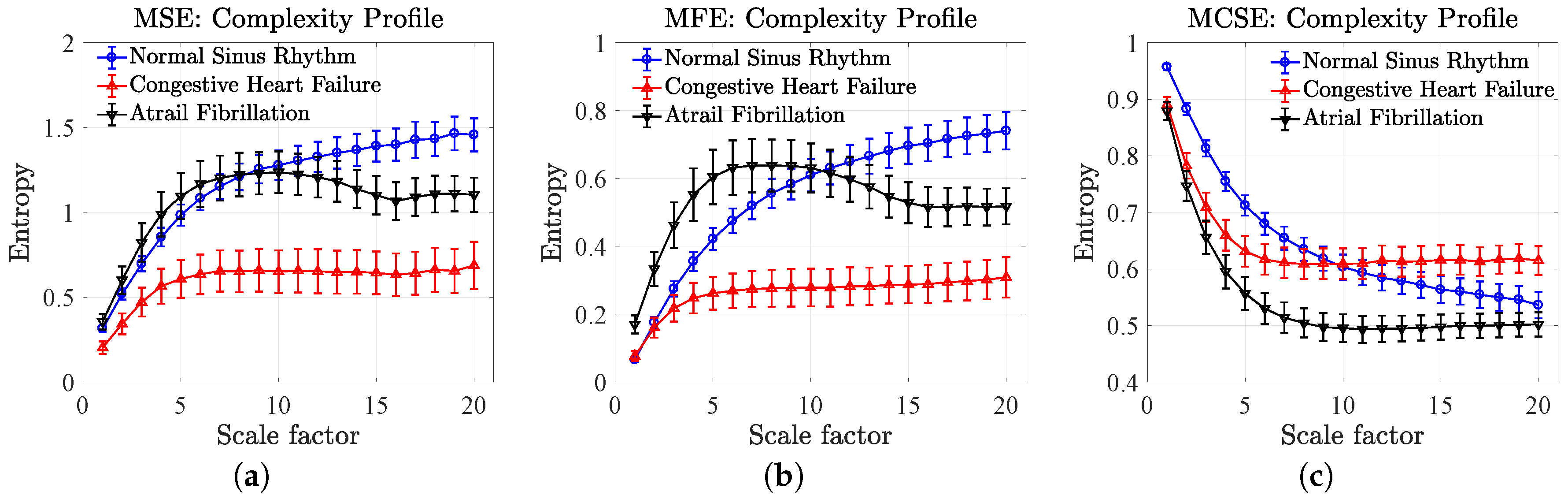
  • The MSE resulted in equal complexity (overlapped mean entropies) for the NSR and the AF, which were higher than the complexity of the CHF at the first scale factor. When increasing the scale factor, the complexity of the three HRVs increased toward the largest scale factor, where the order of degrees of complexity from high to low corresponds to the NSR, AF and CHF.
  • The MFE resulted in equal complexity (overlapped mean entropies) for both the NSR and CHF, which were higher than the complexity of the AF at the first scale factor. When increasing the scale factor, the complexity of the three HRVs increased toward the largest scale factor, where the degrees of complexity from high to low correspond to the NSR, AF and CHF, analogous to the results of the MSE.
  • The MCSE resulted in equal structural complexity measures for both the CHF and AF (overlapped mean entropies), which were higher than the complexity of the NRS at the first scale factor. When increasing the scale factor, the complexity of the three HRVs decreased, and, at the largest scale factor, the degrees of structural complexity from high to low correspond to the CHF, NRS and AF.
Based on the “Complexity Loss Theory”(CLT) [40], the highest degree of complexity is deemed to correspond to the NRS (normal healthy subjects), while the other health conditions are deemed to exhibit lower complexity (pathology or aging) [18,40]. However, this hypothesis is based on degrees of irregularity, whereas our proposed MCSE quantifies structural complexity based on degrees of self-correlation, for which the CHF exhibits highest self-correlated complexity (followed by the NRS and AF). Our proposed measures therefore still admits the interpretation within the concept of the CLT, but with a new definition “pathology exhibits loss in self-uncorrelated complexity”. In other words, pathology exhibits an increase in self-correlated complexity. Additionally, even though the MCSE yields results which are in contrast to the results from the MSE and MFE, we can still see the good separation of mean entropies among the three cardiac conditions in all approaches.
The future work on the CSE and the MCSE will be related to the issues of: (i) baseline wander of a time series; (ii) extending a limited range of entropy values, currently in [0,1]. Within the first issue, we can eliminate an offset of a time series by subtracting its median, as described in Algorithm 3; however, the baseline wander is likely to contain some non-stationary components usually found in real-world signals. This requires more advanced nonlinear techniques to remove such a baseline for the improvement of the calculation of the angular distance. Regarding the second issue, although the CSE and the MCSE result in entropy values between 0 to 1 that can be utilized as a standard range for the comparison of complexity among different signals, this may limit the ability to quantify more profound degrees of complexity of a variety of signals that exhibit high degrees of nonlinear chaos. This is in contrast with the SE, MSE, FE and MFE, which have no maximum bound on the value of estimated entropy. However, unlike the proposed CSE, these approaches are vulnerable to the undefined entropy values when applied to a short time series. In future work, we will also examine the robustness of the CSE and MCSE to spikes and erratic peaks, and will investigate the performances of the CSE and MCSE over a variety of real-world recordings, such as biomedical data and financial data.

Acknowledgments

The work of Danilo P. Mandic was supported by the Engineering and Physical Sciences Research Council (EPSRC), grant reference: EESB-I38012.

Author Contributions

Theerasak Chanwimalueang conceived the cosine similarity entropy algorithm, and Theerasak Chanwimalueang and Danilo P. Mandic designed the simulation tests and methods. Theerasak Chanwimalueang and Danilo P. Mandic analyzed the data. Both authors contributed to writing of the manuscript and commented on the manuscript at all stages. Both authors have read and approved the final manuscript.

Conflicts of Interest

The authors declare no conflict of interest.

Appendix A. Autoregressive Models

To evaluate the performances of the SE, FE and CSE approaches, we generated two groups of AR models: (i) AR(1) with nine varying correlation coefficients and (ii) nine orders of AR processes with the pre-defined correlation coefficients. For the first group, AR(1) models driven by random noise were synthesized using 20 independent realizations of 10,000 samples. Each realization consisted of nine varying coefficients of the AR(1) processes generated as
x ( t ) = α 1 x ( t 1 ) + ε ( t ) ,
where ε ( t ) N ( 0 , 1 ) and α 1 [ 0.1 , 0.2 , 0.3 , 0.4 , 0.5 , 0.6 , 0.7 , 0.8 , 0.9 ] .
For the second group, p-th order AR processes driven by random noise were synthesized using 20 independent realizations of 10,000 samples, given by
x ( t ) = i = 1 p α i x ( t i ) + ε ( t ) ,
where ε ( t ) N ( 0 , 1 ) , p is the AR order increasing from 1 to 9 and α i represents the pre-defined correlation coefficients of the i-th order as shown in Table A1.
Table A1. The pre-defined correlation coefficients used for the nine orders of the AR(p) processes.
Correlation Coefficient α 1 α 2 α 3 α 4 α 5 α 6 α 7 α 8 α 9
AR(1)0.5--------
AR(2)0.50.25-------
AR(3)0.50.250.125------
AR(4)0.50.250.1250.0625-----
AR(5)0.50.250.1250.06250.0313----
AR(6)0.50.250.1250.06250.03130.0156---
AR(7)0.50.250.1250.06250.03130.01560.0078--
AR(8)0.50.250.1250.06250.03130.01560.00780.0039-
AR(9)0.50.250.1250.06250.03130.01560.00780.00390.0019
Note that, with the selected correlation coefficients, both groups of the generated AR models were stable and stationary, which can be seen in Figure A1.
Figure A1. Two groups of synthetic AR processes used for evaluating the performances of the SE, FE and CSE approaches. (a) the first 300 samples from AR(1) processes with nine varying coefficients of correlation ( α 1 ) and the driving WGN input; (b) the first 300 samples of the AR(1)–AR(9) processes with the pre-defined correlation coefficients and the driving WGN input, giving signals with the degrees of freedom of the underlying generation system ranging from 1 to 9.
Entropy 19 00652 g0a1

Appendix B. Heart Rate Variability Database

One-hour RR intervals of the three cardiac pathologies; normal sinus rhythm (NSR), congestive heart failure (CHF) and atrial fibrillation (AF), were extracted from the Physiobank database [41]. The beat annotations (RR intervals) of the NSR and CHF database were obtained by the automated detector with manual review and correction, while the beat annotations of the AF database were only obtained by automated detector. For the NSR database, we obtained 18 RR intervals of subjects who had no significant arrhythmia. The subjects included 5 men, aged 26 to 45, and 13 women, aged 20 to 50. For the CHF database, we selected the first 20 RR intervals from the total of 29 subjects with congestive heart failure (New York Heart Association (NYHA) classes I, II, and III), who aged from 34 to 79. The subjects included eight men and two women; the gender is not known for the remaining 21 subjects. For the AF database, we obtained 20 RR intervals from the total of 25 subjects, with no information about the age and gender [42]. An example of the RR intervals of the three cardiac conditions within 225 s is shown in Figure A2.
Figure A2. Example of the RR intervals (RRI) of the three cardiac conditions over 225 s duration. Top: RRI of the normal sinus rhythm database (in blue); Middle: RRI of the congestive heart failure database (in red); Bottom: graph represents the atrial fibrillation (in black). Observe the highest degrees of correlation (fewer random components) can be observed from the RRI of the CHF, while the lowest degrees of correlation (more random components) can be observed from the RRI of the AF.
Entropy 19 00652 g0a2

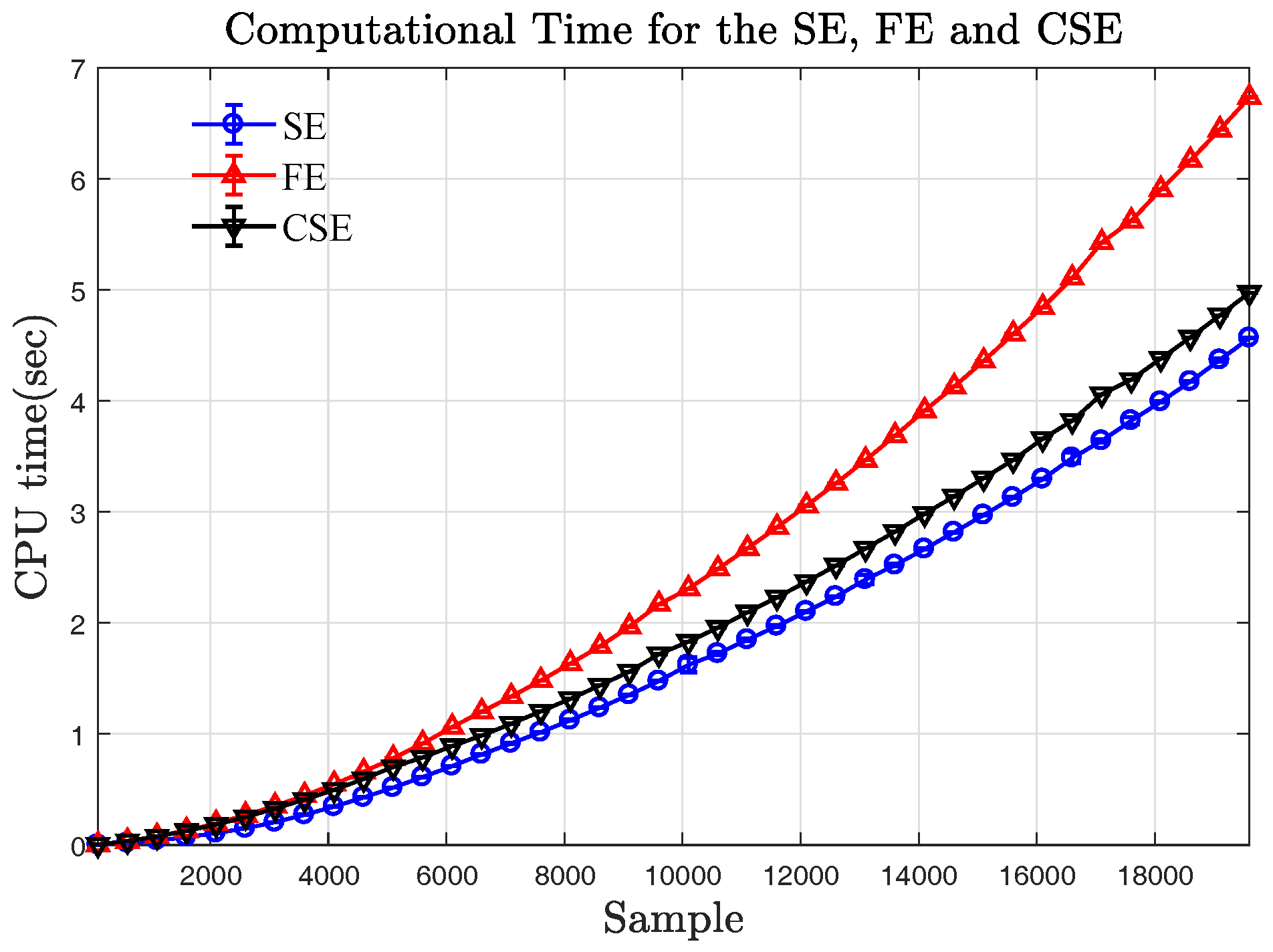
Appendix C. Computational Time

The SE, FE and CSE algorithms were implemented using Matlab 2017b (MathWorks, Inc., Natick, MA, USA) for comparing their performance in terms of computational time (CPU time). We generated 10 independent realizations of 40 incremental sample sizes (100:500:20,000) for WGN to evaluate the three entropy algorithms with the following selected parameters: m = 2 , τ = 1 , r S E = r F E = 0.15 , r C S E = 0.07 and η = 2 . We ran the Matlab codes of the three entropy algorithms under the 64-bit Windows 7 platform (Microsoft Corporation, Redmond, WA, USA) on a personal computer with the Intel 3.40-GHz Intel(R) Core(TM) i7-3370 CPU (Intel Corporation, Santa Clara, CA, USA) and 24-GB RAM. Figure A3 shows mean CPU times (with their SD) used by the three entropy approaches. Observe that for small sample sizes of data, from 100 to 6000 samples, the three approaches used similar mean CPU times (similar performance), while for large sample sizes of data, from 8000 to 20,000 samples, mean CPU times used for the FE approach were higher than the other two entropy approaches, and the SE performed slightly faster than the CSE (at data size of 19,600 samples, the mean CPU times used for the FE, MCE and SE were 6.733, 4.973 and 4.565 s). The slow operation of the FE is due to the CPU task of reserving a large memory size in the step of declaring a float vector variable for the fuzzy similarities (see Step 3 of Algorithm 2), whereas the SE and CSE require only a small size of memory for declaring a Boolean vector variable obtained from the compared distances with a selected tolerance value (see Step 3 of Algorithm 1 and Step 4 of Algorithm 3).
Figure A3. Computational time for the SE, FE and CSE algorithms. The 10 independent realizations of 40 incremental sample sizes (100:500:20,000) for WGN are used to evaluate computational time (CPU time) of the three entropy algorithms. Observe that mean CPU times used for the SE and CSE are relatively similar (the SE performs slightly faster than the CSE), while, at the large sample sizes, mean CPU times used for the FE approach are much higher than for the other entropy approaches (the larger the sample size, the slower the computation of the FE approach).
Entropy 19 00652 g0a3

References

  1. Pincus, S.M. Approximate entropy as a measure of system complexity. Proc. Natl. Acad. Sci. USA 1991, 88, 2297–2301. [Google Scholar] [CrossRef] [PubMed]
  2. Pincus, S.M. Assessing serial irregularity and its implications for health. Ann. N. Y. Acad. Sci. 2001, 954, 245–267. [Google Scholar] [CrossRef] [PubMed]
  3. Takens, F. Detecting Strange Attractors in Turbulence. In Dynamical Systems and Turbulence; Rand, D., Young, L.S., Eds.; Springer: Berlin/Heidelberg, Germany, 1981; pp. 366–381. [Google Scholar]
  4. Packard, N.H.; Crutchfield, J.P.; Farmer, J.D.; Shaw, R.S. Geometry from a time series. Phys. Rev. Lett. 1980, 45, 52–56. [Google Scholar] [CrossRef]
  5. Gautama, T.; Mandic, D.P.; Van Hulle, M.M. The delay vector variance method for detecting determinism and nonlinearity in time series. Phys. D 2004, 190, 167–176. [Google Scholar] [CrossRef]
  6. Richman, J.S.; Moorman, J.R. Physiological time-series analysis using approximate entropy and sample entropy. Am. J. Physiol. 2000, 278, H2039–H2049. [Google Scholar]
  7. Alcaraz, R.; Abásolo, D.; Hornero, R.; Rieta, J. Study of sample entropy ideal computational parameters in the estimation of atrial fibrillation organization from the ECG. Comput. Cardiol. 2010, 37, 1027–1030. [Google Scholar]
  8. Wu, S.D.; Wu, C.W.; Lin, S.G.; Wang, C.C.; Lee, K.Y. Time series analysis using composite multiscale entropy. Entropy 2013, 15, 1069–1084. [Google Scholar] [CrossRef]
  9. Molina-Picó, A.; Cuesta-Frau, D.; Aboy, M.; Crespo, C.; Miró-Martínez, P.; Oltra-Crespo, S. Comparative study of approximate entropy and sample entropy robustness to spikes. Artif. Intell. Med. 2011, 53, 97–106. [Google Scholar] [CrossRef] [PubMed]
  10. Lake, D.E.; Richman, J.S.; Griffin, M.P.; Moorman, J.R. Sample entropy analysis of neonatal heart rate variability. Am. J. Physiol. 2002, 283, R789–R797. [Google Scholar] [CrossRef] [PubMed]
  11. Chen, W.; Wang, Z.; Xie, H.; Yu, W.; Chen, W.; Wang, Z.; Xie, H.; Yu, W. Characterization of surface EMG signal based on fuzzy entropy. IEEE Trans. Neural Syst. Rehabil. Eng. 2007, 15, 266–272. [Google Scholar] [CrossRef] [PubMed]
  12. Xie, H.B.; He, W.X.; Liu, H. Measuring time series regularity using nonlinear similarity-based sample entropy. Phys. Lett. A 2008, 372, 7140–7146. [Google Scholar] [CrossRef]
  13. Chen, W.; Zhuang, J.; Yu, W.; Wang, Z. Measuring complexity using FuzzyEn, ApEn, and SampEn. Med. Eng. Phys. 2009, 31, 61–68. [Google Scholar] [CrossRef] [PubMed]
  14. Xie, H.B.; Guo, J.Y.; Zheng, Y.P. Using the modified sample entropy to detect determinism. Phys. Lett. A 2010, 374, 3926–3931. [Google Scholar] [CrossRef]
  15. Liang, Z.; Wang, Y.; Sun, X.; Li, D.; Voss, L.J.; Sleigh, J.W.; Hagihira, S.; Li, X. EEG entropy measures in anesthesia. Front. Comput. Neurosci. 2015, 9, 16. [Google Scholar] [CrossRef] [PubMed]
  16. Gan, C.; Learmonth, G. Comparing entropy with tests for randomness as a measure of complexity in time series. arXiv, 2015; arXiv:stat.ME/1512.00725. [Google Scholar]
  17. Trifonov, M. The structure function as new integral measure of spatial and temporal properties of multichannel EEG. Brain Inform. 2016, 3, 211–220. [Google Scholar] [CrossRef] [PubMed]
  18. Costa, M.; Goldberger, A.L.; Peng, C. Multiscale entropy analysis of complex physiologic time series. Phys. Rev. Lett. 2002, 89, 6–9. [Google Scholar] [CrossRef] [PubMed]
  19. Costa, M.; Peng, C.K.; Goldberger, A.L.; HauSDorff, J.M. Multiscale entropy analysis of human gait dynamics. Phys. A 2003, 330, 53–60. [Google Scholar] [CrossRef]
  20. Costa, M.; Goldberger, A.L.; Peng, C.K. Multiscale entropy analysis of biological signals. Phys. Rev. E 2005, 71, 21906. [Google Scholar] [CrossRef] [PubMed]
  21. Costa, M.; Ghiran, I.; Peng, C.K.; Nicholson-Weller, A.; Goldberger, A.L. Complex dynamics of human red blood cell flickering: Alterations with in vivo aging. Phys. Rev. E 2008, 78, 20901. [Google Scholar] [CrossRef] [PubMed]
  22. Carter, T. An Introduction to Information Theory and Entropy. Available online: http://astarte.csustan.edu/~tom/SFI-CSSS/info-theory/info-lec.pdf (accessed on 30 September 2017).
  23. Steele, M.J. The Cauchy-Schwarz Master Class: An Introduction to the Art of Mathematical Inequalities; The Mathematical Association of America: Washington, DC, USA, 2004. [Google Scholar]
  24. Deza, E.; Deza, M.M. Encyclopedia of Distances; Springer: Berlin/Heidelberg, Germany, 2009. [Google Scholar]
  25. Kryszkiewicz, M. The Triangle Inequality Versus Projection onto a Dimension in Determining Cosine Similarity Neighborhoods of Non-negative Vectors. In Rough Sets and Current Trends in Computing; Yao, J., Yang, Y., Słowiński, R., Greco, S., Li, H., Mitra, S., Polkowski, L., Eds.; Springer: Berlin/Heidelberg, Germany, 2012; pp. 229–236. [Google Scholar]
  26. Kryszkiewicz, M. The Cosine Similarity in Terms of the Euclidean Distance. In Encyclopedia of Business Analytics and Optimization; IGI Global: Hershey, PA, USA, 2014; pp. 2498–2508. [Google Scholar]
  27. Abbad, A.; Abbad, K.; Tairi, H. Face Recognition Based on City-block and Mahalanobis Cosine Distance. In Proceedings of the International Conference on Computer Graphics, Imaging and Visualization (CGiV), Beni Mellal, Morocco, 29 March–1 April 2016; pp. 112–114. [Google Scholar]
  28. Senoussaoui, M.; Kenny, P.; Stafylakis, T.; Dumouchel, P. A Study of the cosine distance-based mean shift for telephone speech diarization. IEEE/ACM Trans. Audio Speech Lang. Process. 2014, 22, 217–227. [Google Scholar] [CrossRef]
  29. Sahu, L.; Mohan, B.R. An Improved K-means Algorithm Using Modified Cosine Distance Measure for Document Clustering Using Mahout with Hadoop. In Proceedings of the International Conference on Industrial and Information Systems (ICIIS), Gwalior, India, 15–17 December 2014; pp. 1–5. [Google Scholar]
  30. Ji, J.; Li, J.; Tian, Q.; Yan, S.; Zhang, B. Angular-similarity-preserving binary signatures for linear subspaces. IEEE Trans. Image Process. 2015, 24, 4372–4380. [Google Scholar] [CrossRef] [PubMed]
  31. Pearson, K. Note on regression and inheritance in the case of two parents. Proc. R. Soc. Lond. 1985, 58, 240–242. [Google Scholar] [CrossRef]
  32. Stigler, S.M. Francis Galton’s account of the invention of correlation. Stat. Sci. 1989, 4, 73–79. [Google Scholar] [CrossRef]
  33. Székely, G.J.; Rizzo, M.L.; Bakirov, N.K. Measuring and testing dependence by correlation of distances. Ann. Stat. 2007, 35, 2769–2794. [Google Scholar] [CrossRef]
  34. Josh Patterson, A.G. Deep Learning a Practitioner’s Approach, 1st ed.; O’Reilly Media: Sevastopol, CA, USA, 2015; p. 536. [Google Scholar]
  35. Pincus, S.M.; Goldberger, A.L. Physiological time-series analysis: What does regularity quantify? Am. J. Physiol. 1994, 266, H1643–H1656. [Google Scholar] [PubMed]
  36. Kaffashi, F.; Foglyano, R.; Wilson, C.G.; Loparo, K.A.; Kenneth, A.L. The effect of time delay on approximate & sample Entropy calculations. Phys. D 2008, 237, 3069–3074. [Google Scholar]
  37. Richman, J.S.; Lake, D.E.; Moorman, J. Sample entropy. Methods Enzymol. 2004, 384, 172–184. [Google Scholar] [PubMed]
  38. Gautama, T.; Mandic, D.P.; Van Hulle, M.M. A Differential Entropy Based Method for Determining the Optimal Embedding Parameters of a Signal. In Proceedings of the IEEE International Conference on Acoustics, Speech, and Signal Processing, Hong Kong, China, 6–10 April 2003; Volume 6, pp. 29–32. [Google Scholar]
  39. Shalizi, C.R. Methods and Techniques of Complex Systems Science: An Overview. In Complex Systems Science in Biomedicine; Deisboeck, T.S., Kresh, J.Y., Eds.; Springer: Boston, MA, USA, 2006; pp. 33–114. [Google Scholar]
  40. Lipsitz, L.A.; Goldberger, A.L. Loss of complexity and aging. Potential applications of fractals and chaos theory to senescence. J. Am. Med. Assoc. 1992, 267, 1806–1809. [Google Scholar] [CrossRef]
  41. Goldberger, A.L.; Amaral, L.A.; Glass, L.; HauSDorff, J.M.; Ivanov, P.C.; Mark, R.G.; Mietus, J.E.; Moody, G.B.; Peng, C.K.K.; Stanley, H.E. PhysioBank, PhysioToolkit, and PhysioNet: Components of a new research resource for complex physiologic signals. Circulation 2000, 101, E215–E220. [Google Scholar] [CrossRef] [PubMed]
  42. Moody, G.B.; Mark, R.G. A new method for detecting atrial fibrillation using RR intervals. In Proceedings of the International Conference on Computers in Cardiology, Aachen, Germany, 4–7 October 1983; pp. 227–230. [Google Scholar]
Figure 1. Geometric interpretation of the Chebyshev and angular distances in Cartesian coordinates. (a) Chebyshev distance of two embedding vectors x 1 ( m ) and x 2 ( m ) , with embedding dimensions m = 2 and m = 3 . The Chebyshev distance represents the coordinate-wise maximum amplitude difference of the two embedding vectors; (b) the angular distance of embedding vectors x 1 ( m ) and x 2 ( m ) with m = 2 and m = 3 ; the angles α 1 , 2 ( m ) and the angular distance between the two embedding vectors are calculated using Equations (6) and (7).
Entropy 19 00652 g001
Figure 2. Geometric interpretation of similar patterns in three-dimensional phase space reconstruction. The embedding vector, x ( 3 ) is reconstructed from an Electrocardiogram (ECG) time series using m = 3 and τ = 1 . (a) normalized raw ECG time series; (b) Chebyshev distance; similar patterns are located inside the red sphere spanned by the radius (tolerance), r S E , from a particular embedding vector x i ( 3 ) located at the center; (c) angular distance; similar patterns are captured inside the cone beam projected from the origin to a particular embedding vector x i ( 3 ) , where the angle of the cone beam is equal to the angular distance (tolerance), r C S E . Observe that the area of the similarity derived from the angular distance method is independent of amplitude levels, unlike the Chebyshev distance method. This means that the angular distance can detect similar structural patterns even though the amplitudes of the elements of a particular embedding vector are scaled.
Entropy 19 00652 g002
Figure 3. Selection of the tolerance parameter for the Cosine Similarity Entropy (CSE) algorithm. (a) standard Shannon entropy curve as a function of the probability of a selected event ( P r ( X = 1 ) ) when using 1-bit data; (b) Four CSE curves for White Gaussian Noise (WGN), 1 / f noise, autoregressive processes AR(1) and AR(2), when varying r C S E from 0.01 to 0.99.
Entropy 19 00652 g003
Figure 4. Comparison of the entropy curves over a varying embedding dimension, m, using the Sample Entropy (SE), the fuzzy entropy (FE) and CSE approaches. The 30 independent realizations with 1000 samples were generated for each of the four synthetic signals; WGN, 1 / f noise, AR(1) and AR(2). The mean entropies with their standard deviations are plotted against the embedding dimension. (a) results of the SE; (b) results of the FE; and (c) results of the CSE.
Entropy 19 00652 g004
Figure 5. Comparison of the entropy curves over varying sample sizes using the SE, FE and CSE approaches. The 30 independent realizations, with sample sizes ranging from 10 to 5000 samples, were generated for each of the four synthetic signals; WGN, 1 / f noise, AR(1) and AR(2). The mean entropies with their standard deviations are plotted against data length N. (a) results of the SE; (b) results of the FE; (c) results of the CSE. Observe that, at the sample size of 1000, the CSE yielded the smallest SD of mean entropies of all synthetic signals (see Table 1).
Entropy 19 00652 g005
Figure 6. Comparison of the complexity profiles of the four synthetic signals, WGN, 1 / f noise, AR(1) and AR(2), using the Multiscale Sample Entropy (MSE), the multiscale fuzzy entropy (MFE) and Multiscale Cosine Similarity Entropy (MCSE) approaches. The 20 independent realizations with 10,000 samples were generated for each of the four synthetic signals. The mean entropies with their standard deviations are plotted against the coarse-grained scales. (a) results of the MSE; (b) results of the MFE; (c) results of the MCSE. Observe that the MCSE produces very consistent and correct behaviors in terms of the degrees of structural complexity, especially for large scales where the 1 / f noise exhibits correctly the highest complexity (long-term correlation), unlike the MSE and MFE in plots (a,b).
Entropy 19 00652 g006
Figure 7. Comparison of the complexity profiles of AR(1) processes with a varying (correlation) coefficient α 1 , using the MSE, MFE and MCSE approaches. The 20 independent realizations with 10,000 samples of WGN were generated as a driving noise for each of the nine AR(1) with a varying correlation coefficient α 1 ( α 1 = [ 0.1 , 0.2 , , 0.8 , 0.9 ] (see more detail in Appendix A). The mean entropies with their standard deviations are plotted against the coarse-grained scales. (a) results of the MSE; (b) results of the MFE; (c) results of the MCSE. Observe that the complexity order of all AR(1) processes estimated from the MCSE is consistent over all scale factors, while the MSE and MFE produced different and inconsistent complexity values ordered from small to large AR(1) coefficients. The AR(1) processes exhibit a single degree of freedom in their structural complexity, and only the proposed MCSE was able to reveal physical insight.
Entropy 19 00652 g007
Figure 8. Comparison of the complexity profiles of AR(p) processes, where p is the AR order ranging from 1 to 9, using the MSE, MFE and MCSE approaches. The 20 independent realizations with 10,000 samples of WGN were generated as a driving noise for each of the nine AR(p) processes with pre-defined correlation coefficients (for details see Appendix A). The mean entropies with their standard deviations are plotted against the coarse-grained scales. (a) results of the MSE; (b) results of the MFE and (c) results of the MCSE. Observe the complexity order of all AR(1) processes estimated from the MCSE is consistent over all scale factors, while the MSE and MFE produce mixed complexity order from small ( ϵ > 4 ) to large scale factors.
Entropy 19 00652 g008
Figure 9. Comparison of the complexity profiles of heart rate variability using the MSE, MFE and MCSE approaches. Three conditions of heart rate variability were considered: (i) normal sinus rhythm; (ii) congestive heart failure and (iii) atrial fibrillation, which were obtained from the Physionet database (for more details, see Appendix B). Mean entropies and their standard errors are plotted against the coarse-grained scales. (a) results of the MSE; (b) results of the MFE; (c) results of the MCSE. Notice that the MCSE yields highest long-term correlation for the Congestive Heart Failure (CHF) and lower degrees of long-term correlation for the Normal Sinus Rhythm (NSR) and Atrial Fibrillation (AF). These correct highest degrees of correlation (fewer random components) can also be observed from the raw signals of the CHF as shown in Figure A2, while the lowest degrees of correlation (more random components) can be observed from the raw signals of the AF.
Entropy 19 00652 g009
Table 1. Standard deviation (SD) of entropy values of WGN, 1 / f noise, AR(1) and AR(2) with a sample sizes of N = 1000 . SD of entropy values of WGN, 1 / f noise, AR(1) and AR(2) with a sample sizes of N = 1000 . The entropy values were estimated using the SE, FE and CSE approaches for a comparison of the variation of the entropy values.
Approach/Type of SignalSE
(SD of Entropies)
FE
(SD of Entropies)
CSE
(SD of Entropies)
WGN0.05860.01460.0011
1 / f noise0.09750.08800.0287
AR(1)0.06560.05050.0267
AR(2)0.09820.05800.0401
Table 2. Recommended parameters ranges for the SE, FE and CSE algorithms.
Parameter/ApproachSEFECSE
Tolerance (r)0.1–0.25 [7]0.1–0.3 [11]0.05–0.2
Embedding dimension (m)1–31–102–5
Min. sample size (N) for WGN & 1 / f noise30050100
Min. sample size (N) for AR(1) & AR(2)700500700

