


Abstract
We consider the problem of learning a Bayesian network structure given n examples and the prior probability based on maximizing the posterior probability. We propose an algorithm that runs in time and that addresses continuous variables and discrete variables without assuming any class of distribution. We prove that the decision is strongly consistent, i.e., correct with probability one as . To date, consistency has only been obtained for discrete variables for this class of problem, and many authors have attempted to prove consistency when continuous variables are present. Furthermore, we prove that the “” term that appears in the penalty term of the description length can be replaced by to obtain strong consistency, where is arbitrary, which implies that the Hannan–Quinn proposition holds.
1. Introduction
In this paper, we address the problem of learning a Bayesian network structure from examples.
For sets of random variables, we say that A and B are conditionally independent given C if the conditional probability of A and B given C is the product of the conditional probabilities of A given C and B given C. A Bayesian network (BN) is a graphical model that expresses conditional independence (CI) relations among the prepared variables using a directed acyclic graph (DAG). We define a BN by the DAG with vertexes and directed edges , where edge directs from j to k, via minimal parent sets , , such that the distribution is factorized by:
First, suppose that we wish to know whether two random binary variables X and Y are independent (hereafter, we write ). If we have n pairs of actually emitted examples and know the prior probability p of , then it would be reasonable to maximize the posterior probability of given and . If we assume that the probabilities and are parameterized by , and and that the prior probabilities and over the probabilities and of , and are available, respectively, then we can construct the quantities:
In this setting, maximizing the posterior probability of given examples w.r.t. the prior probability p is equivalent to deciding if and only if:
The decision based on (1) is strongly consistent, i.e., it is correct with probability one as [1] (see Section 3.1 for the proof). We say that a model selection procedure satisfies weak consistency if the probability of choosing the correct model goes to unity as n grows (probability convergence) and that it satisfies strong consistency if the probability one is assigned to the set of infinite example sequences that choose the correct model, except for at most finite times (almost sure convergence). In general, strong consistency implies weak consistency, but the converse is not true [2]. In any model selection, in particular for large n, the correct answer is required. If continuous variables are present, the BN structure learning is not easy, and strong consistency is hard to obtain.
The same scenario is applied to the case in which X and Y take values from finite sets A and B rather than .
Next, suppose that we wish to know the factorization of three random binary variables : , , , , , , , , and . If we have n triples of actually emitted examples and know the prior probabilities over the eleven factorizations, then it would be reasonable to choose the one that maximizes:
to maximize the posterior probability of the factorization given , and . For example, between the last two distributions, we choose the last if and only if:
In fact, for example, we can check that the factorizations:
in Figure 1a–c share the same form , and we say that they share the same Markov-equivalent class. On the other hand, the factorization
in Figure 1d has nothing to share with the same Markov equivalent class, except itself. In the case of three variables, there are 25 DAGs, but they reduce to the eleven Markov equivalent classes.
Figure 1.
Markov-equivalent classes (a–d).

The method that maximizes the posterior probability is strongly consistent [1] (see Section 3.1 for the proof), and a scenario with two and three variables as above can be extended to cases with N variables in a straightforward manner, if the variables are discrete.
In this paper, we consider the case when continuous variables are present. The idea is to construct measures , and over , and for continuous ranges X and Y to make the decision whether based on:
The main problem is whether the decision is strongly consistent. Many authors have attempted to address continuous variables. For example, Nir Friedman [3] experimentally demonstrated the construction of a genetic network based on expression data using the E-Malgorithm. However, the variables were assumed to be linearly related and included Gaussian noise, and the dataset was not sufficiently fit to the model. Imoto et al. [4] improved the model such that the relation is expressed by B-spline curves rather than lines. However, all of the authors, including Friedman and Imoto, failed to maximize the posterior probability, and thus, the decision is not consistent. This paper proves that the decision based on (2) and its extension for general is strongly consistent.
In any Bayesian approach of BN structure learning, whether continuous variables are present or not, the procedure consists of two stages:
- (1)
- Compute the local scores for the nonempty subsets of ; for example, if , the seven quantities are obtained; and
- (2)
- Find a BN structure that maximizes the global scores among the candidate BN structures; there are at most DAGs in the case of N variables; for example, if , the eleven quantities are computed and a structure with the largest is chosen.
Note that the second stage does not care about whether each variable is continuous or not. In this paper, we mainly discuss about the performance of the first stage. The number of local scores to be computed can be saved, although it is generally exponential with N. We consider the problem inSection 3.3.
On the other hand, Zhang, Peters, Janzing and Scholkopf [5] proposed a BN structure learning method using conditional independence (CI) tests based on kernel statistics. However, for the CI test that is close to the Hilbert–Schmidt information criterion (HSIC), it is very hard to simulate the null distribution. They only proposed to approximate it by a Gamma distribution, but no consistency, is obtained because the threshold of the statistical test is not correct in practice. Furthermore, for the independence test approach, it often results in conflicting assertions of independence for finite samples. In particular, for small samples, the obtained DAG sometimes contain a directed loop. The Bayesian approach we consider in this paper does not suffer from the inconvenience, because we seek a structure that maximizes the global score [6].
Another contribution of this paper is identifying the border between consistency and non-consistency in learning Bayesian networks. For discrete X, maximizing is equivalent to minimizing the description length [1]:
where is the empirical entropy of (we write when is bounded by a constant) and α is the cardinality of set X. The problem at hand is whether the term is the minimum function of n for ensuring strong consistency. If is replaced by two (AIC), we cannot obtain consistency. We prove that with is the minimum for strong consistency based on the law of iterated logarithms. The same property is known as the Hannan–Quinn principle [7], and similar results have been obtained for autoregression, linear regression [8] and classification [9], among others. The derivation in this paper does not depend on these previous results. The Hannan–Quinn principle will also be applied to continuous variables.
This paper is organized as follows. Section 2.1 introduces the general concept of learning Bayesian network structures based on maximizing the posterior probability, and Section 2.2 discusses the concept of density functions developed by Boris Ryabko [10] and extended by Suzuki [11]. Section 3 presents our contributions: Section 3.1 proves the Hannan–Quinn property in the current problem, andSection 3.2 proves consistency when continuous variables are present. Section 4 concludes the paper by summarizing the results and states the paper's significance in the field of model selection.
2. Preliminaries
2.1. Learning the Bayesian Structure for Discrete Variables and Its Consistency
We choose , such that and by , where X is the set from which X takes its values. Let , and let be the frequency of in , . It is known that the following quantities satisfies (3) [12]:
where Γ is the Gamma function, and Stirling's formula has been applied. Thus, for , from the law of large numbers, converges to with probability one as , such that:
with probability one as .
Moreover, from the law of large numbers, with probability one as ,
(Shannon–McMillan–Breiman [13]). This proves that there exists a (universal measure), such that for any probability P over the finite set X,
with probability one as , where we write . The same property holds for:
and:
where , and are the empirical entropies of and , and and are the numbers of occurrences of and in and , respectively.
Thus, we have:
with probability one as . However, if and only if . Hence, if , the value of is positive with probability one as . However, how can we detect when ? cannot be exactly zero with probability one as .
However, when X and Y are discrete, the estimation based on is consistent: if , the value of is not greater than zero with probability one as . For example, the decision based on (1) is strongly consistent because the values of and are negligible for large n, and asymptotically, (1) is equivalent to .
In Section 3.1, we provide a stronger result of consistency and a more intuitive and elegant proof.
In general, if N variables exist (), we must consider two cases: and, where and P are the probabilities based on the correct and estimated factorizations and denotes the Kullback–Leibler divergence between and P. If , then:
if and only if in and in P.
The same property holds for three variables ():
with probability one as , and if and only if . Then, we can show if and only if , with probability one as (see Section 3.1). For example, between the seventh and eleventh factorizations, if and , then we choose the seventh and eleventh, respectively. In fact,
for large n, because diminishes.
Then, the decision is correct with probability one as . Similarly, we calculate:
and:
where . In general, for N variables, given P and , we have all of the CI statements for each of them, and if and only if the CI statements in P imply those in ; in other words, P induces an I-map, which is not necessarily minimal.
Note that for any subsets of , we can construct the estimation , with , and obtain consistency, i.e., we will have the correct CI statements, where c may be empty.
Table 1 depicts whether or for each and P. For example, if the factorizations of and P are the fourth and sixth, then from the table. In general, if and only if is realized using the factorization and an appropriate parameterset for P.
Table 1.
Three-variable case: or : “+” and “0” denote and , respectively.
2.2. Universal Measures for Continuous Variables
In this section, we primarily address continuous variables.
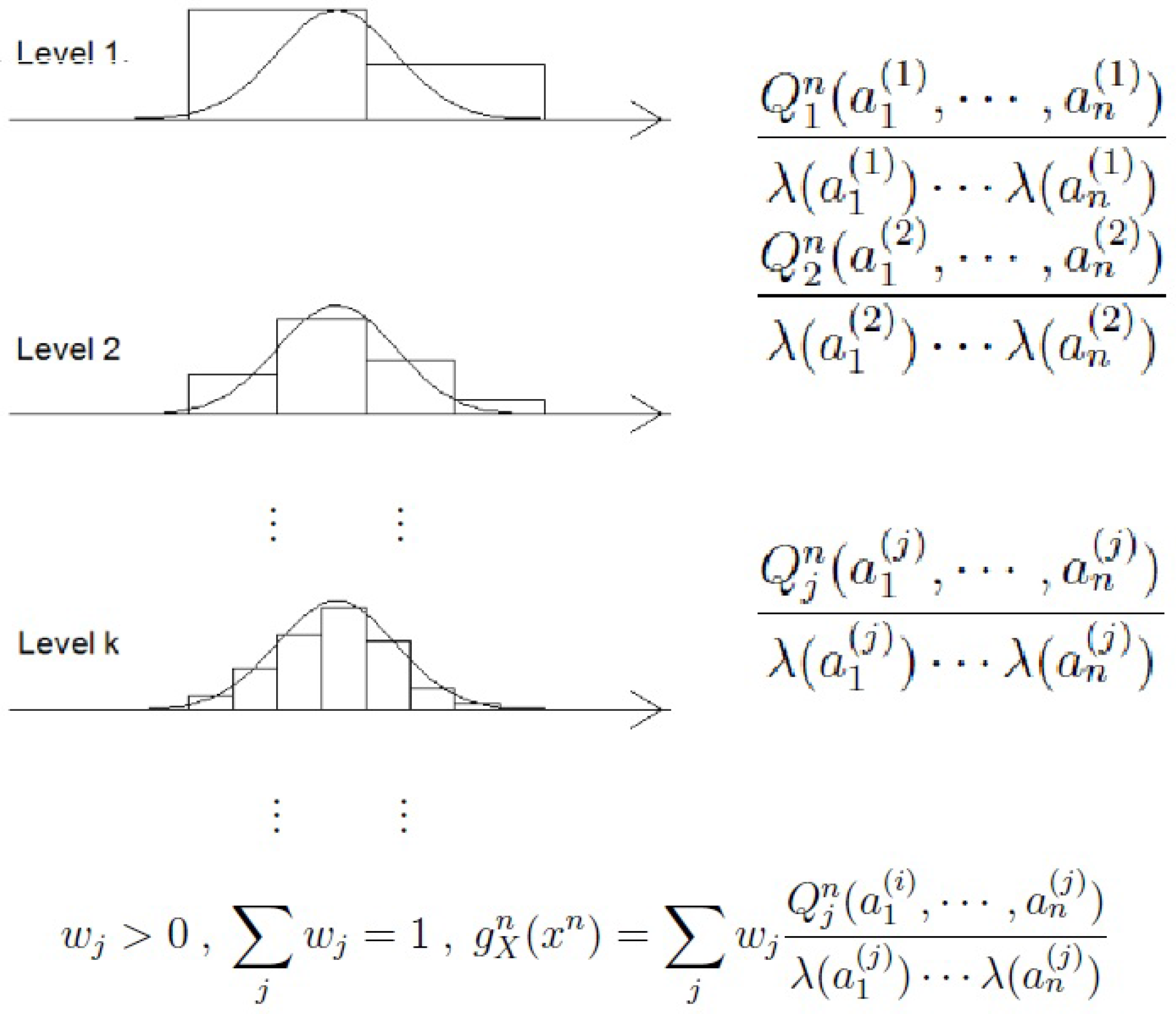
Let be such that , and let be a refinement of . For example, suppose that the random variable X takes values in , and we generate a sequence as follows:
For each j, we quantize each into the , such that . For example, for , is quantized into . Let λ be the Lebesgue measure (width of the interval). For example, and .
Note that each is a finite set. Therefore, we can construct a universal measure w.r.t. a finite set for each j. Given , we obtain a quantized sequence for each j and use it to compute the quantity:
for each j. If we prepare a sequence of positive reals , such that and , we can compute the quantity:
Moreover, let be the true density function and for and if . We may consider to be an approximated density function assuming the quantization sequence (Figure 2). For the given , we define and .
Figure 2.
Quantization at level k:
Thus, we have the following proposition, which is a continuous version of the universality (4) that was proven in Section 2.1.
Proposition 1 ([10]). For any density function f, such that as ,
as with probability one, where is the Kullback–Leibler divergence between and .
The same concept is applied to the case where no density function exists [11] in the usual sense (w.r.t. the Lebesgue measure λ). For example, suppose that we wish to estimate a distribution over the positive integers N. Apparently, N is not a finite set and has no density function. We consider the quantization sequence : , , , ..., , ....
For each k, we quantize each into a , such that . For example, for , is quantized into . Let η be a measure, such that:
The measure for closed interval a gives:
if and are the minimum and maximum integers in a, and evaluates each bin width in a nonstandard way. For example, and . For multiple variables, we compute the measure by:
Note that each is a finite set, and we construct a universal measure w.r.t. a finite set for each k. Given , we obtain a quantized sequence for each k, such that we can compute the quantity:
for each k. If we prepare a sequence of positive reals , such that and , we can compute the quantity . In this case, for ( with may take any arbitrary value) is considered to be a generalized density function (w.r.t. the measure η).
In general, if implies for the Borel sets (the Borel sets w.r.t. R being the set consisting of the sets generated via a countable number of union, intersection and set difference from the closed intervals of R [2]), we state that P is absolutely continuous w.r.t. η and that there exists a density function w.r.t. η (Radon–Nikodym [2]).
The following proposition addresses generalized densities and eliminates the condition as in Proposition 1.
Proposition 2 ([11]). For any generalized density function ,
as with probability one.
Proposition 1 assumes a specific quantization sequence, such as . The universality holds for the densities that satisfy as [10]. However, in the proof of Proposition 2, a universal quantization, such that as for any density , was constructed [11].
3. Contributions
3.1. The Hannan and Quinn Principle
We know that is at most with probability one as when because the decision based on (1) is strongly consistent.
In this section, we prove a stronger result: let:
We show that the quantity is at most rather than, when :
Theorem 1. If :
with probability one as for any .
In order to show the claim, we approximate by with , where , , are mutually independent random variables with mean zero and variance , such that:
Then, from the law of iterated logarithms below (Lemma 1) [2], it will be proven that is almost surely upper-bounded by for any and each , which implies Theorem 1 because:
(see the Appendix for the details of the derivation).
Lemma 1 ([2]). Let be random variables that obey an identical distribution with zero mean and unit variance, and . Then, with probability one,
Theorem 1 implies the strong consistency of the decision based on (1). However, a stronger statement can be obtained:
Theorem 2. We define , , and by:
and:
Then, the decision based on:
is strongly consistent.
Proof. We note two properties:
- is equivalent to (7); and
If , then from Theorem 1 and the first property, we have almost surely. If almost surely holds, then the value in the second property should be no greater than zero, which means that . This completes the proof. ☐
Theorem 2 is related to the Hannan and Quinn theorem [7] for model selection. To obtain strong consistency, they proved that rather than is sufficient for the penalty terms of autoregressive model selection. Recently, several authors have proven this in other settings, such as classification [9] and linear regression [8].
3.2. Consistency for Continuous Variables
Suppose that we wish to estimate the distribution over in Section 2.2. The set is not a finite set and has no density function.
Because is a finite set, we can construct a universal measure for :
If we prepare the sequence such that , , we obtain the quantity:
In this case, the (generalized) density function is obtained via:
where ( takes arbitrary values for and ), where is the conditional distribution function of X given .
In general, we have the following result:
Proposition 3 For any generalized density function f:
as with probability one.
The measures and are computed using (A) and (B) of Algorithm 1, where the value of K is the number of quantizations, and and denote the approximated scores using finite quantization of level K.
| Algorithm 1 Calculating gn. | |
| (A) Input xn ∈ An, Output | |
| 1. | For each , |
| 2. | For each and each , |
| 3. | For each , |
| (a) , | |
| (b) for each | |
| i. Find from | |
| ii. | |
| iii. | |
| 4. | |
| (B) Input and , Output | |
| 1. | For each , |
| 2. | For each and each and , |
| 3. | For each |
| (a) , , , | |
| (b) for each | |
| i. Find and from and | |
| ii. | |
| iii. | |
| 4. | |
Propositions 1–3 are obtained for large K. However, we can prepare only a finite number of quantizations. Furthermore, if n is small, then the number of examples that each bin contains is small, and we cannot estimate the histogram well. Therefore, given n, K must be moderately sized, and we recommend to set because the number of examples contained in a bin decreases exponentially with increasing depth, where m is the number of variables in the local score. For example, and for (A) and (B), respectively. Algorithm 1 (A)(B) of do not guarantee anything for the theoretical property assured in Proposition 3 and Theorems 3–5 for finite K, however, as K grows, consistency holds.
In Step 3(a) of Algorithm 1(A)(B), we calculate from and not from , which means that the computational time required to obtain from is . Thus, the total computation times of Algorithm 1 (A)(B) are at most .
In Step 3(b) of Algorithm 1(A), we compute for and :
if is quantized into , .
For the memory requirements, we require exponential orders of K. However, because we set , the computational time and memory requirements are at most and for Algorithm 1(A)(B).
Based on the same notion, we can construct , , , from examples , and , and Propositions 2 and 3 hold for three variables.
Theorem 3. With probability one as :
Proof. From Propositions 2 and 3 for two and three variables and the law of large numbers, we have:
with probability one, which completes the proof. ☐
From the discussion in Section 2.1, even when more than two variables are present, if , we can choose rather than P with probability one as .
Now, we prove that the continuous counterpart of the decision based on (1) is strongly consistent:
Theorem 4. With probability one as :
where p is the prior probability of .
Proof: Suppose that . Then, the conditional mutual information between X and Y given Z is positive, and from Theorem 3, the estimator converges to a positive value with probability one as ; thus, holds almost surely. Suppose that . The discrete variables X and Y are conditionally independent given Z if and only if:
with probability one as for any constant , even if c does not coincide with the prior probability p. If and Z are continuous, we quantize , and into , and . Thus, for each and l, we have:
with probability one as . Thus, if we divide both sides by:
and take summations of both sides over , we have:
with probability one, where we have assumed because of , which completes the proof.
Note that even if either X or Y is discrete, the same conclusion will be obtained. The generalized density functions cover the discrete distributions as a special case.
From the discussion in Section 2.1, even when more than two variables are present, if , we can choose rather than P with probability one as .
Let ,, and take the same values of , , and , except that the terms in , , and are replaced by , respectively, where is arbitrary. Then, we obtain the final result:
Theorem 5. With probability one as :
This paper focuses on the theoretical aspects of the BN structure learning, in particular for consistency when continuous variables are present. For the details of the practical matters we deal with in this section, see the conference paper [14].
3.3. The Number of Local Scores to be Computed
We refer the conditional independence (CF) score w.r.t. X and Y given Z to the left of (8). Suppose we follow the fastest Bayesian network structure learning due to [6]: let be the optimal parent set of contained in for and its local score. Then, we can obtain:
For each , the sinks:
and the parent sets:
For each fixed pair (, maximizing the local score and maximizing the CF score w.r.t. and , given W are equivalent. In other words,
for .
On the other hand, from [15,16], we know that the relationship between the complexity term and the likelihood term gives tight bounds on the maximum number of parents in the optimal BN for any given dataset. In particular, the number of elements in each parent set is at most for and . Hence, the number for computing the CF scores is much less than exponentialwith N.
4. Concluding Remarks
In this paper, we considered the problem of learning a Bayesian network structure from examples and provided two contributions.
First, we found that the terms in the penalty terms of the description length can be replaced by to obtain strong consistency, where the derivation is based on the law of iterated logarithms. We claim that the Hannan and Quinn principle [7] is applicable to this problem.
Second, we constructed an extended version of the score function for finding a Bayesian network structure with the maximum posterior probability and proved that the decision is strongly consistent even when continuous variables are present. Thus far, consistency has been obtained only for discrete variables, and many authors have been seeking consistency when continuous variables are present.
Consistency has been proven in many model selection methods that maximize the posterior probability or, equivalently, minimize the description length [1]. However, almost all such methods assume that the variables are either discrete or that the variables obey Gaussian distributions. This paper proposed an extended version of the MDL/Bayesian principle without assuming such constraints and proved its strong consistency in a precise manner, which we believe provides a substantial contribution to the statistics and machine learning communities.
Appendix: Proof of Theorem 1
Hereafter, we write P(X = x|Z = z) and P(Y = y|Z = z) simply as P(x|z) and P(y|z) respectively, for x ∈ X, y ∈ Y and z ∈ Z. We find that the empirical mutual information:
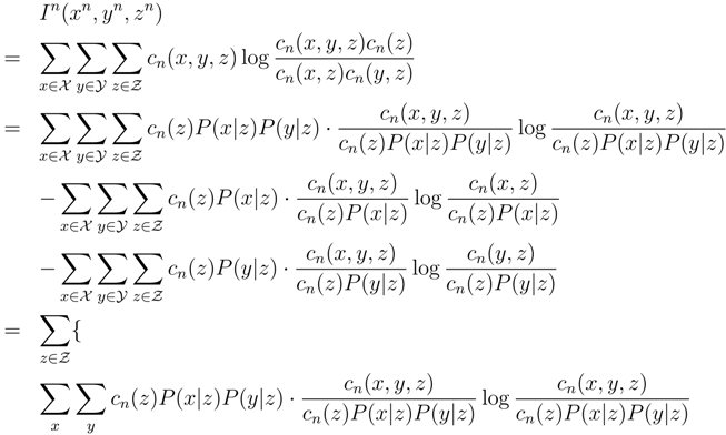

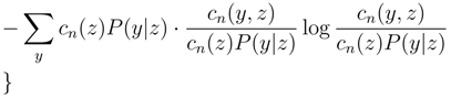 is approximated by
  with:
with:
 where the difference between them is zero with probability one as n → ∞, and (1 + t)log(1 + t) = t + t2/2 − t3/{6[1 + δ(t)t]2} with 0 < δ(t) < 1 and:
 has been applied for (11), (12) and (13), respectively. Furthermore, we derive:
 where V = (Vxy)x ∈ X, and y ∈ Y with
  and u and v are the column vectors
 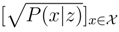 and
and 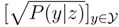 , respectively. Hereafter, we arbitrarily fix z ∈ Z. Let U = (u[0], u[1], …, u[α − 1]), with u[0] = u and W = (w[0], w[1], …, w[β − 1], with w[0] = w being eigenvectors of
  and
and  , where Em is the identity matrix of dimension m.
with:
and u and v are the column vectors and , respectively. Hereafter, we arbitrarily fix z ∈ Z. Let U = (u[0], u[1], …, u[α − 1]), with u[0] = u and W = (w[0], w[1], …, w[β − 1], with w[0] = w being eigenvectors of and , where Em is the identity matrix of dimension m.Then, tuVw = 0, and for = (u[1], …, u[α − 1] and = (w[1], …, w[β − 1], we have:
 and:
and:
 If we note that UtU = tUU = Eα and WtW = tWW = Eβ, we obtain:
 and find that (14) becomes:
 with rij := tu[i]Vw[j]. Then, we can see:
 and that the (α − 1) × (β − 1) matrix consists of mutually independent elements rij with i = 1, …, α − 1 and j = 1, …, β − 1: E[rij] = 0, and:
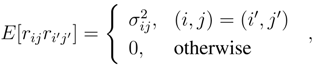 where is the variance of rij and the expectation of , so that (15) implies:
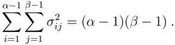
If we define for each x ∈ X and y ∈ Y and for i = 1, …, n:
 where u[i] = (u[i,x])x ∈ X and w[j] = (w[y,j])y ∈ Y, then we can check E[Zi,j,k] = 0 and V[Zi,j,k] = 1, where expectation E and variance V are with respect to the examples Xn = xn and Yn = yn, and I(A) takes one if the event A is true and zero otherwise. We can easily check:
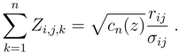
We consider applying the obtained derivation to Lemma 1. From (17), we obtain:
 which means that (14) is upper bounded by(1 + ϵ)(α − 1)(β − 1)log log n with probability one as n → ∞ for any ϵ > 0, from (16). This completes the proof of Theorem 1.
References
- Rissanen, J. Modeling by shortest data description. Automatica 1978, 14, 465–471. [Google Scholar] [CrossRef]
- Billingsley, P. Probability & Measure, 3rd ed.; Wiley: New York, NY, USA, 1995. [Google Scholar]
- Friedman, N.; Linial, M.; Nachman, I.; Pe'er, D. Using Bayesian networks to analyze expression data. J. Comput. Biol. 2000, 7, 601–620. [Google Scholar] [CrossRef] [PubMed]
- Imoto, S.; Kim, S.; Goto, T.; Aburatani, S.; Tashiro, K.; Kuhara, S.; Miyano, S. Bayesian network and nonparametric heteroscedastic regression for nonlinear modeling of genetic network. J. Bioinform. Comput. Biol. 2003, 1, 231–252. [Google Scholar] [CrossRef] [PubMed]
- Zhang, K.; Peters, J.; Janzing, D.; Scholkopf, B. Kernel-based Conditional Independence Test and Application in Causal Discovery. In Proceedings of the 2011 Uncertainty in Artificial Intelligence Conference, Barcelona, Spain, 14–17 July 2011; pp. 804–813.
- Silander, T.; Myllymaki, P. A simple approach for finding the globally optimal Bayesian network structure. In Proceedings of the 22nd Conference on Uncertainty in Artificial Intelligence, Arlington, Virginia, 13–16 July 2006; pp. 445–452.
- Hannan, E.J.; Quinn, B.G. The Determination of the Order of an Autoregression. J. R. Stat. Soc. B 1979, 41, 190–195. [Google Scholar]
- Suzuki, J. The Hannan–Quinn Proposition for Linear Regression, Int. J. Stat. Probab. 2012, 1, 2. [Google Scholar]
- Suzuki, J. On Strong Consistency of Model Selection in Classification. IEEE Trans. Inf. Theory 2006, 52, 4767–4774. [Google Scholar] [CrossRef]
- Ryabko, B. Compression-based Methods for Nonparametric Prediction and Estimation of Some Characteristics of Time Series, IEEE Trans. Inform. Theory 2009, 55, 4309–4315. [Google Scholar] [CrossRef]
- Suzuki, J. Universal Bayesian Measures. In Proceedings of the 2013 IEEE International Symposium on Information Theory, Istanbul, Turkey, 7–12 July 2013; pp. 644–648.
- Krichevsky, R.E.; Trofimov, V.K. The Performance of Universal Encoding. IEEE Trans. Inf. Theory 1981, 27, 199–207. [Google Scholar] [CrossRef]
- Cover, T.M.; Thomas, J.A. Elements of Information Theory, 2nd ed.; Wiley: New York, NY, USA, 1995. [Google Scholar]
- Suzuki, J. Learning Bayesian Network Structures When Discrete and Continuous Variables Are Present. In Proceedings of the 2014 Workshop on Probabilistic Graphical Models, 17–19 September 2014; Springer Lecture Notes on Artificial Intelligence. Volume 8754, pp. 471–486.
- Suzuki, J. Learning Bayesian belief networks based on the minimum description length principle: An efficient algorithm using the B&B technique. In Proceedings of the 13th International Conference on Machine Learning (ICML'96), Bari, Italy, 3–6 July 1996; pp. 462–470.
- De Campos, C.P.; Ji, Q. Efficient Structure Learning of Bayesian Networks using Constraints. JMLR 2011, 12, 663–689. [Google Scholar]
- Akaike, H. A new look at the statistical model identification. IEEE Trans. Autom. Control 1974, 19, 716–723. [Google Scholar] [CrossRef]
- Judea, P. Probabilistic Reasoning in Intelligent Systems: Networks of Plausible Inference; Morgan-Kaufmann: San Mateo, CA, USA, 1988. [Google Scholar]
© 2015 by the authors; licensee MDPI, Basel, Switzerland. This article is an open access article distributed under the terms and conditions of the Creative Commons Attribution license (http://creativecommons.org/licenses/by/4.0/).