A Community-Based Approach to Identifying Influential Spreaders

Abstract

Identifying influential spreaders in complex networks has a significant impact on understanding and control of spreading process in networks. In this paper, we introduce a new centrality index to identify influential spreaders in a network based on the community structure of the network. The community-based centrality (CbC) considers both the number and sizes of communities that are directly linked by a node. We discuss correlations between CbC and other classical centrality indices. Based on simulations of the single source of infection with the Susceptible-Infected-Recovered (SIR) model, we find that CbC can help to identify some critical influential nodes that other indices cannot find. We also investigate the stability of CbC.

1. Introduction

Fast and accurate identification of influential spreaders in a network is essential to the acceleration of information diffusion, inhibition of gossip and spread of a virus. During the two decades from the emergence of network science to its current dramatic developments [1–5], the measurement of node importance has been the key concern of researchers, and many indicators that are used to describe node importance have been successively proposed [6].

Previously, node importance ranking measurement indexes based on the structure of the network were determined from local and global properties of the network, the position of the network and random walks [7]. Various recent studies have shown that the methods for ranking the importance of nodes based on community structure characteristics are also of realistic significance, and more interesting “singular nodes” can be excavated from the ranking result of influence via the spreading process.

An index based on the local properties of a network that is represented by the degree of the node basically considers the information of the node and its neighbors. The index calculation is simple, and it can be used for large-scale networks. Degree is the most intuitive; a node with greater degree can impact more neighbors. Meanwhile, as a node in a susceptible state, it is at a higher risk of infection by its neighbors [8–10]. Chen et al. [11] considered the degree information of the nearest neighbors and the second nearest neighbors, and they also defined the importance ranking of local centrality to the network nodes. Centola studied the behavior spreading process of online social networks and found that the behavior spreads farther and faster across clustered-lattice networks than across corresponding random networks. An influential spreader is associated with the clustering of the nodes [12]; it was found by Ugander et al. from the evolution characteristics of friends’ relation networks on Facebook that the absolute number of neighbors was not the determinant influencing the importance of a node; rather, the determinant was the number of connected components between neighbors [13].

A node importance ranking index based on global network properties basically considers the global information of the network. The accuracy of this type of index is generally higher, but the time complexity of computation is also higher. For example, betweenness is defined as the number of shortest paths that pass through the node, so the betweenness of the node represents the “busyness” of the node [14]. To some extent, betweenness of the node can reflect the importance of information in the spreading process [15]. Closeness [16] is used to measure the capability of nodes in the network to influence other nodes through the network. It can also be calculated by the average distance from a given starting node to all other nodes in the network. Consequently, it can be considered as a measure of how long it will take to spread information from a given node to other reachable nodes in the network. Eigenvector [17,18] is an important index evaluating the importance of a node. Eigenvector considers the prestige of a single node as the combination of the prestige of all other nodes from the perspectives of the position or prestige of nodes in the network.

In 2010, Kitsak and others [19] studied the application of K-core decomposition in identifying the influential spreaders of the network. K-core is the connected component formed by nodes whose degree is not less than k in the network. All of the nodes that belong to K-core but do not belong to (K + 1)-core are the nodes in K-shell. Therefore, all of the nodes in the network use the index K-shell Ks to describe their importance in the spreading process. Obviously, the degree of a node contained in the Ks-shell inevitably satisfies k ≥ Ks. The use of Ks to measure the influence of a node on the spreading process is now widely recognized as a measurement method [20]. In recent years, many scholars have extended and improved K-core. For example, Zeng et al. [21] considered the information of the Ks degree of removed nodes after Ks decomposition, and they proposed the mixed degree decomposition method (MMD). Garas et al. [22] developed Ks decomposition for weighted networks. Liu et al. [23] comprehensively considered the target node K-shell and its distance from the largest K-core of the network, which overcomes the defect that it was unable to accurately measure the importance of a node as a result of having the same value of Ks for such a large number of nodes in the network after K-shell decomposition. In addition, Hou et al. [24] considered the impact of three different indicators, including degree, betweenness and K-core, on the importance of nodes, and they used the Euler distance formula to calculate the combined action of these three different indicators.

The importance ranking method based on random walks is basically based on the PageRank technology of link relations between webpages. As the link relationship between webpages can be explained as the correlation and support between webpages, so too can the importance of the webpage be judged. Typical methods include the Hypertext-Induced Topic Search (HITS) algorithm [25] proposed by Kleinberg, the PageRank algorithm [26] used by Google and LeaderRank [27] proposed recently by Lv Linyuan et al. Then in 2014, Weighted LeaderRank [28] as an improvement method was presented by Li et al. Current research on identifying influential spreaders, many interesting conclusions were successively put forward, such as the role of clustering [29] by Chen D-B et al. who also proposed to improve the identification of influential spreaders by the path diversity [30].

As the actual network usually has a community structure, nodes in each community connect with each other closely, while the connection between the communities is relatively scattered [31]. Therefore, the community property of a node can be used for the ranking of importance. For example, Hu et al. [32] proposed an improved index based on the centrality of K-shell and the community structure and also validated it on the SIR Model. The number of communities that can be linked by a node (V-community) is defined as the measurement index of the “variety of neighbors” for the node [33].

Obviously, only considering the number of communities that are directly linked by the node (V-community) is not comprehensive enough. There are two deficient aspects. First, the importance measurement method based on the network community structure completely depends on the result of community division, while different community division algorithms have different results, especially for large-scale networks. Second, the size of each community in the network is significantly different, and this is not taken into consideration by V-community. This paper improves on these deficiencies and proposes another index, Community-based Centrality (CbC), which is used to identify the influential spreaders based on the network community structure.

2. A Community-Based Centrality Index

Most natural networks are found and divided naturally into communities or modules [34]. Moreover, one of the more intriguing issues prevailing throughout the last decade of network science is how to research the topological community structure. The inspiration for considering the importance of nodes within the community structure was the theory of “the strength of weak ties” by Mark Granovetter in 1973 [35]. He surprisingly found that, more often than not, weak connections lead to strong interactions. This means a long-range connection may lead to a stronger interaction between two nodes than will short connections of neighboring nodes. Interesting enough, this paper turned out to be one of the most important papers with the highest impact in the field of social science today [36]. From the view of network science, the network can be presented by a set V of nodes and a set E of edges, connected together as a graph denoted by G = (V, E), where the total number of nodes is N = |V| and that of edges is M = |E|. Each edge e ∈ E is connected to one pair of nodes, one at each end. Clearly, (i, j) indicates an edge between two connected nodes i and j. Thus, an adjacency matrix with N nodes and M edges is described by A = (a_ij)_{N × N}.

2.1. Community-Based Centrality

We can assume that each node has two different types of links: strong links and weak links. A strong link is defined as an edge between nodes that are in the same community, and a weak link is defined as an edge that links two nodes belonging to different communities. Because the connections are much stronger in a certain community than the ones between different communities, the importance of nodes can be calculated by both characteristics of edges and the sizes of communities. For example, in a social network, if a person has many friends in different fields, we can assume that he plays an important role in his social circle. Furthermore, on one hand, he can gain a variety of information from his friends more conveniently, and, on the other hand, he can diffuse information around his circle much more quickly. As a side note here, the number of different fields indicates the variety of friends; however, the amount of friends in each fields cannot be ignored as well. Thus, an index named community-based centrality (CbC) is proposed to calculate the importance of node i via the following formula:

$$Cb{C}_i={\displaystyle \sum _{w=1}^c{d}_{iw}\frac{S_w}{N}}$$

(1)

where c is the number of communities in the network, d_iw is the number of links between node i and other nodes in community w, S_w is the number of nodes in community w (the size of community w). Clearly, we have ${\displaystyle \sum _{w=1}^c{d}_{iw}}=d_i$, where d_i is the degree of node i.

The proposed CbC can be viewed as a generalization of the classical degree centrality. In fact, if the whole network is viewed as a single community, then the CbC of a node reduces to its degree, i.e., CbC_i = d_i. On the other hand, if we view every single node as a community in the network, then the CbC of a node reduces to its normalized degree, i.e., CbC_i = d_i/N.

In recent years, a variety of community discovery algorithms have been proposed [37–41]. Modularity is a commonly used standard to measure the community division quality [41]. A common algorithm based on modularity optimization, the CNM algorithm [42] proposed by Clauset, Newman and Moore, is adopted in this paper. As an illustration example, we consider a network with 21 nodes and 32 edges (Figure 1).

Table 1. Centrality indices of nodes in a simple network.

ID	mc	S	d	Betweenness	Closeness	Eigenvector Centrality	K-shell	CbC
1	1	3	2	0	2.4	0	2	0.428571
2	1	3	6	110.1667	1.75	0.019043	2	1.52381
3	2	4	4	51	2.4	0.069846	3	0.714286
4	2	4	3	0	3.25	0.13232	3	0.571429
5	2	4	3	0	3.25	0.310387	3	0.571429
6	2	4	3	0	3.25	0.67766	3	0.571429
7	3	8	5	37.41667	2.15	0.380233	2	1.666667
8	3	8	1	0	3.1	0.490072	1	0.380952
9	3	8	2	1	2.9	0.490072	2	0.761905
10	3	8	6	58.41667	2	0.069846	2	1.952381
11	3	8	3	2	2.7	0.13232	2	1.142857
12	3	8	4	19.5	2.7	0.310387	2	1.52381
13	3	8	1	0	3.65	0.367273	1	0.380952
14	3	8	3	3.333333	2.75	1	2	1.142857
15	4	6	3	2.083333	2.75	0.162483	2	0.857143
16	4	6	7	63.25	2.15	0.079368	2	1.714286
17	4	6	2	0	3.05	0.386868	2	0.571429
18	4	6	1	0	3.1	0.162483	1	0.285714
19	4	6	1	0	3.1	0.162483	1	0.285714
20	4	6	3	16.83333	2.4	0.519188	2	0.952381
21	1	3	1	0	2.7	0	1	0.142857

lists the CbC and some other centrality indices of nodes in the simple network. The network is divided via CNM algorithm into four communities (c = 4).

Through calculation, the average degree (denoted as <k>) of the network is 3.048, while the degree of node 16 is the maximum, which is 7. The maximum betweenness is shown for node 2, which is 110.1667; node 10 has the maximum CbC, CbC(10) = 1.952381. It can be seen that the nodes with the maximum CbC, degree or betweenness are not the same.

2.2. Experimental Datasets

The experimental data in this paper is conventional datasets [43,44], specific parameters of the networks and sources are presented in

Table 2. Specific statistical parameters for the dataset networks.

Network	N	M	<k>	L	Φ	ρ	Q	c	CC
Facebook	324	2218	13.691	3.054	7	0.042	0.597	27	0.466
Metabolic	453	2025	8.94	2.664	7	0.02	0.416	10	0.655
Email	1133	5451	9.622	3.606	8	0.009	0.521	68	0.220
Power	4941	6594	2.669	18.989	46	0.001	0.932	38	0.107
Router	5022	6258	2.492	6.449	15	0	0.897	62	0.033
Blogcatalog	10312	333983	64.776	2.382	5	0.006	0.238	6	0.463

.

Among them, <k> refers to the average degree of the network, L refers to the average path length, Φ refers to the network diameter, ρ refers to the network density, Q refers to the modularity of the current community division, c refers to the number of communities obtained from the community division of the network through the CNM algorithm proposed in the literature [40], and CC refers to the average clustering coefficient of the network. The topological structures of the dataset networks are presented in Figure 2, in which communities are described by different colors and the CbC of nodes are indicated by the sizes of the individuals.

As schematized in the six subfigures of Figure 2, the large nodes (high CbC) are quite rare in the networks, which are almost decentralized into different communities. Thus, the high CbC nodes can be considered as the community leaders in a sense. Furthermore, in comparison with the other figures above, because the topological structure is clearer, we chose the Facebook network topology for the spreading results presented in the following sections.

To evaluate the effects by different algorithms of community detection methods, some of the common algorithms were used in the supported experiment. It is no doubt that the results of the modularity by each algorithm are basically different even though the numbers of communities are similar. (

Table 3. The modularity (Q), the number of communities (c) by different algorithms of community detection methods proposed in the literatures [40,42,46–50]. The Pearson Correlation Coefficient (r) between spreading capabilities (in the same spreading probability β = 0.05) and CbCs calculated by different algorithms of community detection methods.

Algorithm	Facebook			Metabolic			Email
	Q	c	r	Q	c	r	Q	c	r
CNM1[42]	0.597	27	0.967438	0.416	10	0.824310	0.521	68	0.720225
CNM2	0.530	6	0.869004	0.409	10	0.840384	0.529	8	0.889797
Walk Trap [46]	0.601	25	0.947099	0.349	35	0.869187	0.531	49	0.827893
Multi-level [47]	0.6292197	8	0.841616	0.437	11	0.833422	0.569	11	0.638531
Spin-glass [48,49]	0.6292835	10	0.436205	0.443	13	0.839240	0.581	13	0.895838
LabelPropagation 1 [50]	0.575	11	0.7872296	0.334	5	0.836569	0.528	11	0.770258
LabelPropagation 2	0.607	13	0.945307	0.313	7	0.830448	0.330	8	0.851228
LabelPropagation 3	0.598	11	0.820159	0.340	9	0.844415	0.481	16	0.842951

). In this paper, the Pearson correlation coefficient, the most familiar measure of dependence between two quantities, commonly called simply “the correlation coefficient” [45], was used to measure the correlations between the influence of nodes and the indexes including the CbCs. The Pearson correlation coefficient (denoted r) is a measure of the linear correlation (dependence) between two variables X and Y, giving a value between +1 and −1 inclusive, where 1 is total positive correlation, 0 is no correlation, and −1 is total negative correlation. Thus r is used to measure the degree of correlation between two variables. Where |r| > 0.8, it means extremely strong correlation; Where |r| between 0.6 and 0.8, means strong correlation; Where |r| between 0.4 and 0.6, means moderately related.

In which, CNM algorithm, or the Fast Greedy algorithm, tries to find dense subgraph, also called communities in graphs via directly optimizing a modularity score. The Walk Trap function tries to find densely connected subgraphs, namely communities in a graph via random walks. The algorithm is that short random walks tending into the same community. The Multi-level algorithm implements the multi-level modularity optimization algorithm based on the modularity measure and a hierarchical approach for finding community structure. The Spin-glass algorithm tries to detect communities in graphs by simulated annealing via a spin-glass model. Though the Label Propagation algorithm is fast, even nearly linear time, but the results of detecting were not the same by each time the algorithm was executed independently. The algorithm works by (1) labeling the vertices with unique labels; and (2) updating the labels by majority voting in the neighborhood of the vertex.

Furthermore, in order to present the structures by these methods visually, some representative graphs are drawn (Figure 3).

Based on the community structures by each algorithm, a series CbCs of each nodes in the network can be calculated. Obviously, each set of CbCs would be barely similar to the other set with the basically difference between results by community detection algorithms. However, it is unexpected that the Pearson correlation coefficient r between those sets of CbCs were extraordinary (

Table 4. The analyses of correlations by different algorithms of community detection methods.

Varieties of Pearson correlation coefficient	Facebook	Metabolic	Email
CNM1 and CNM2	0.896228	0.986156	0.866306
CNM1 and Walk Trap	0.972730	0.967388	0.657566
LabelPropagation1 and LabelPropagation3	0.990029	0.998585	0.755279
Multi-level and LabelPropagation1	0.964390	0.984780	0.852465
CNM2 and LabelPropagation2	0.929233	0.961293	0.891828

), namely, the significance of nodes measured by CbC rarely depended on community detection methods. Furthermore, with comparing the Pearson correlation coefficient between CbCs of Facebook network by CNM1 (c = 27) and CNM2 (c = 6), r = 0.896; Metabolic network by LabelPropagation1 (c = 5) and LabelPropagation3 (c = 9), r = 0.999, namely, the number of communities is not the indispensable factor in CbC calculating especially by the same algorithm.

By comparing the experimental results of datasets in Table 3 and Table 4, the qualities of community structures on metabolic network by different community detection algorithms, are rarely better than the ones on email network. Fortunately, the correlations of CbCs are all extremely strong. Thus it can be considered that there is little serious effect by quality of community structure in CbC.

Above all, beyond expectation, different community detection methods can hardly change the overall ranking sorts by CbC. However, as a whole, the results on Facebook network and metabolic network are more significant than on Email network. As a suspect, the accuracy for ranking the influence of nodes would be limited by the topological structure of the network itself.

3. The Correlations Between CbC and Other Indices

3.1. Evaluation With The SIR Model

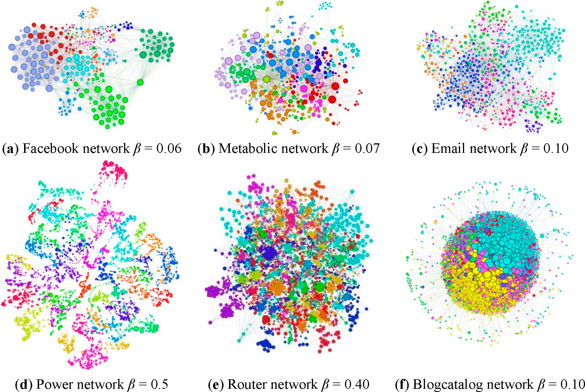
For the investigation of the spreading experiment on the actual network, node i, which is used as the source of infection, can infect the scale of the other nodes to measure the impact of node i. When comparing the impact scale of the node as the initial infection source to other nodes in the network, the greater the number of nodes impacted, the greater the impact of the source node.

We adopt the SIR (Susceptible-Infected-Removed) model for the spreading experiment, i.e., a node infects its neighbors with the probability β, and it is assumed that each infected individual is changed to the “removed” status at a fixed rate γ. In this paper, it is assumed that γ = 1, i.e., in the process of each round of spreading, each infected node only has one chance to infect its neighbors with the probability β, and then the node is “removed”. The initial infection method is monophyletic, and the infection threshold β is set as small as possible; the purpose of this is to make the infection speed slow, and it can also make the selection of the infection source more meaningful. In addition, the number from the experimental result is the expectation value. Even when given two sets of identical conditions, the numbers of infected individuals from two groups of experiment are not the same as a result of the randomness and the small value of the infection probability β. Therefore, we need to regard each node as the initial infection source and take the arithmetic average of 100 independent experiments.

For the experiment, select different values of β according to the scale of different datasets; the selection is based on making the average infected network scale less than 20% and the maximal influence less than 50%. The infection threshold values of networks are provided in

Table 5. The infection threshold values of networks.

Network	Facebook	Metabolic	Email	Power	Router	Blogcatalog
Infection Threshold (β)	0.06	0.07	0.10	–	0.40	0.10
Average Influence	7.7437%	6.2507%	14.9706%	–	10.6013%	7.2571%
Maximal Influence	25.6173%	25.6071%	41.8358%	–	33.8112%	27.4631%

. Because the power network is quite sparse and the average path length (18.989) is much longer than 6, the results of spreading are not as significant as others.

As shown in Figure 4, the influence of every individual is presented by the size of the corresponding node in these topological graphs.

Take the spreading capability of the source node as a measurement standard of the node importance, and compare the importance index between the CbC and other nodes. The results of the experiment are described in a temperature figure in Section 3.2; the temperature’s corresponding value is the number of other nodes infected by the source node.

3.2. Experimental Analysis

With comparing the Pearson correlation coefficient between CbCs (by CNM, Walk trap and Label Propagation) and other classic indexes (

Table 6. The Pearson Correlation Coefficient (r) between CbCs and other classic indexes.

Index	Facebook			Metabolic			Email
	CNM	WT	LP	CNM	WT	LP	CNM	WT	LP
Degree	0.9583	0.9239	0.9404	0.9863	0.9718	0.9962	0.9704	0.8751	0.8809
Betweenness	0.4316	0.4436	0.5000	0.8369	0.8144	0.8566	0.8531	0.7957	0.7920
Closeness	−0.719	−0.727	−0.752	−0.412	−0.442	−0.416	−0.758	−0.736	−0.702
Eigenvector	0.9849	0.9482	0.9466	0.9290	0.9538	0.9409	0.9106	0.8553	0.8801
Ks	0.8622	0.7902	0.8087	0.5992	0.6178	0.5942	0.7940	0.7105	0.6918

), it is clearly reflected that the correlations between CbCs and degree are the extremely strong correlations, so as to eigenvector. Meanwhile, the correlations between CbCs and Ks are strong ones.

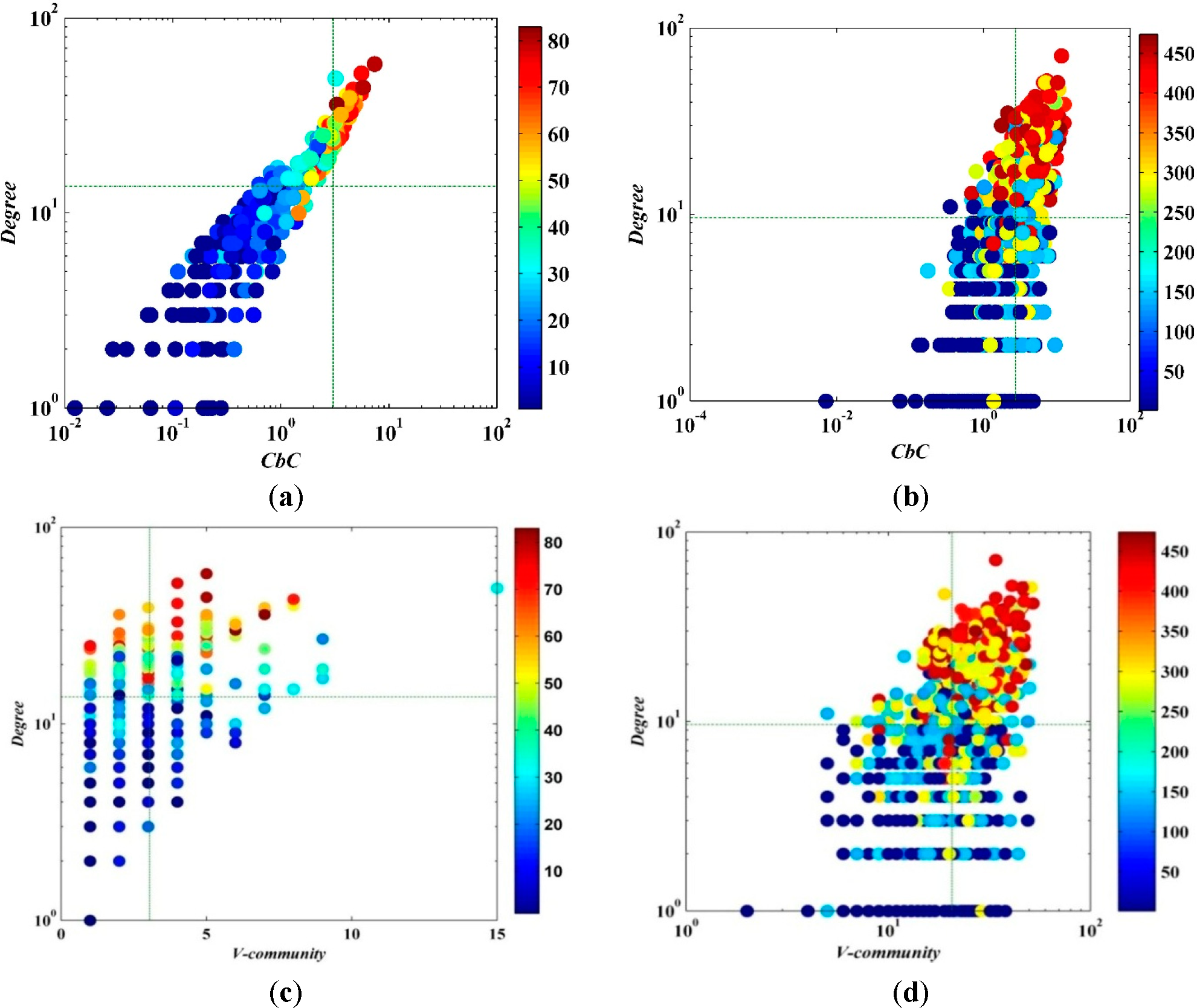
The relation between the CbC and degree of the node illustrated in Figure 5 indicates their obviously positive correlation. The node with the larger degree has a higher CbC. In the Email network, there are quite a number of nodes (as shown in the fourth quadrant of Figure 5b) with high CbC, but its degree is not large. It can be seen from the temperature that a node with large degree and high CbC has strong spreading capability (e.g., the first quadrant). Compare the spreading capability of a node with the same quadrant; it can be seen that, when the degree of the node is close, the node with the high CbC has strong spreading capability. Meanwhile, the insufficiency of using degree to measure the importance can also be seen; some nodes do not have large degrees but do have strong spreading capability, which is clearly shown in Figure 5b. Because calculating CbC (i) requires traversing node i’s neighborhood, the computational complexity of our algorithm is O(n<k>), which grows linearly with the size of a sparse network. Compared with degree centrality (O(n), where n is the number of nodes in the network), CbC can better quantify the influence of nodes, but it has higher computational complexity.

Compared with V-community ((c) and (d) of Figure 5 through Figure 9 at the following part in this paper) presented by the reference [33] in which the graphs in black and white were in the numbers from 6 to 10, the new measurement demonstrates a more statistically significant result.

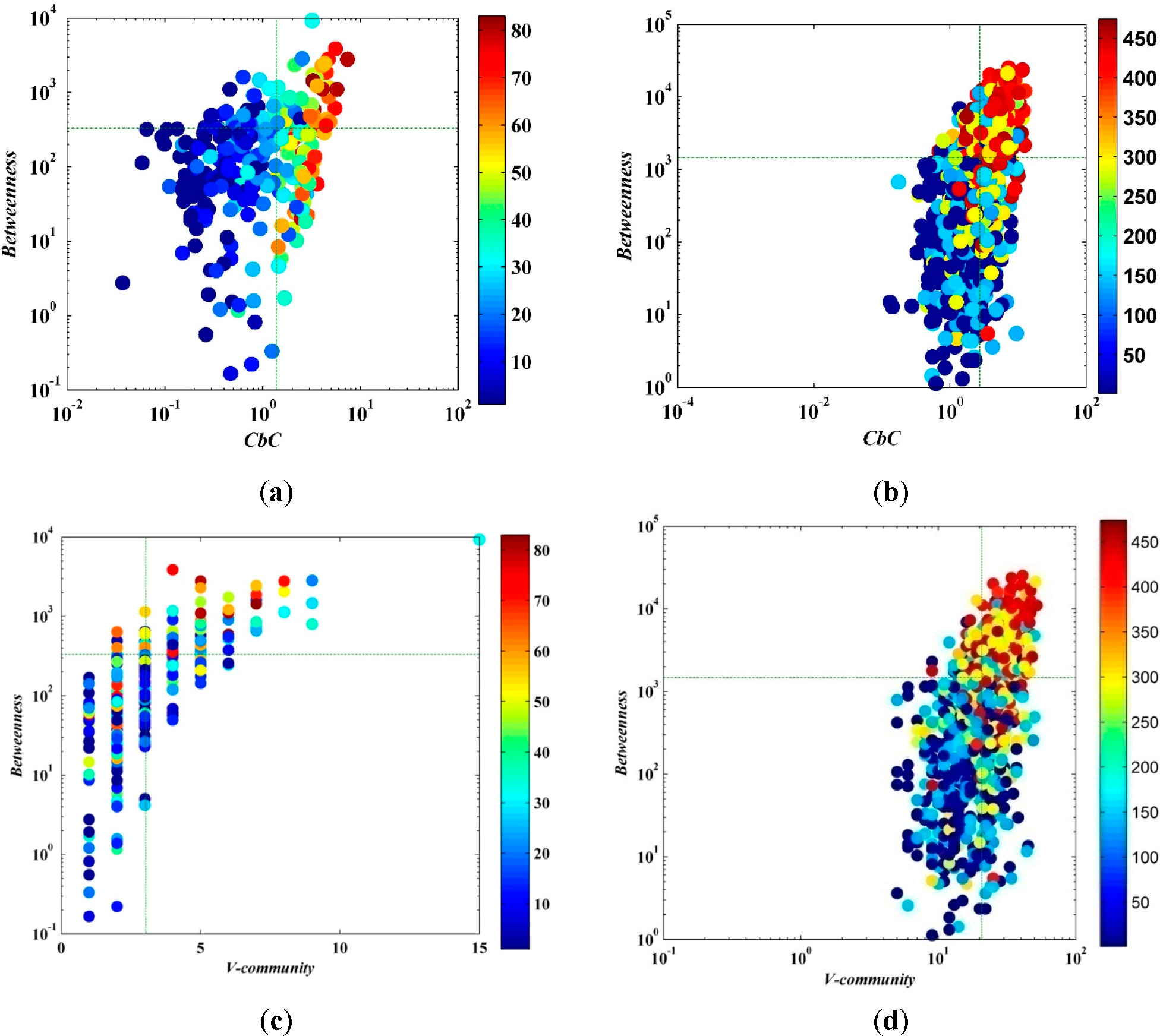
Betweenness is a measure of the centrality of a node in a network and is normally calculated as the fraction of the shortest paths between node pairs that pass through the node of interest. As shown in Figure 6, it can be described from the trend that the CbC and betweenness have a positive correlation. It can be seen from the figure that the node with larger betweenness and higher CbC has stronger spreading capability. Moreover, CbC can better measure the importance of a node compared to betweenness. When the node with higher CbC (e.g., the first and the fourth quadrant), even if the betweenness is small (e.g., the fourth quadrant), the node can still have a spectacular range of influence. However, on the contrary, when the node has large betweenness but lower CbC (e.g., the second quadrant), the number of nodes with strong spreading capability is significantly smaller. In addition, the computational complexity degree of CbC is much lower than that of betweenness (calculating the shortest paths between all pairs of nodes in a network has the complexity O(n³) when using Floyd’s algorithm [51]; for unweighted networks, calculating betweenness centrality requires O(nm) = O(n²<k>) using Brandes’ algorithm [52]).

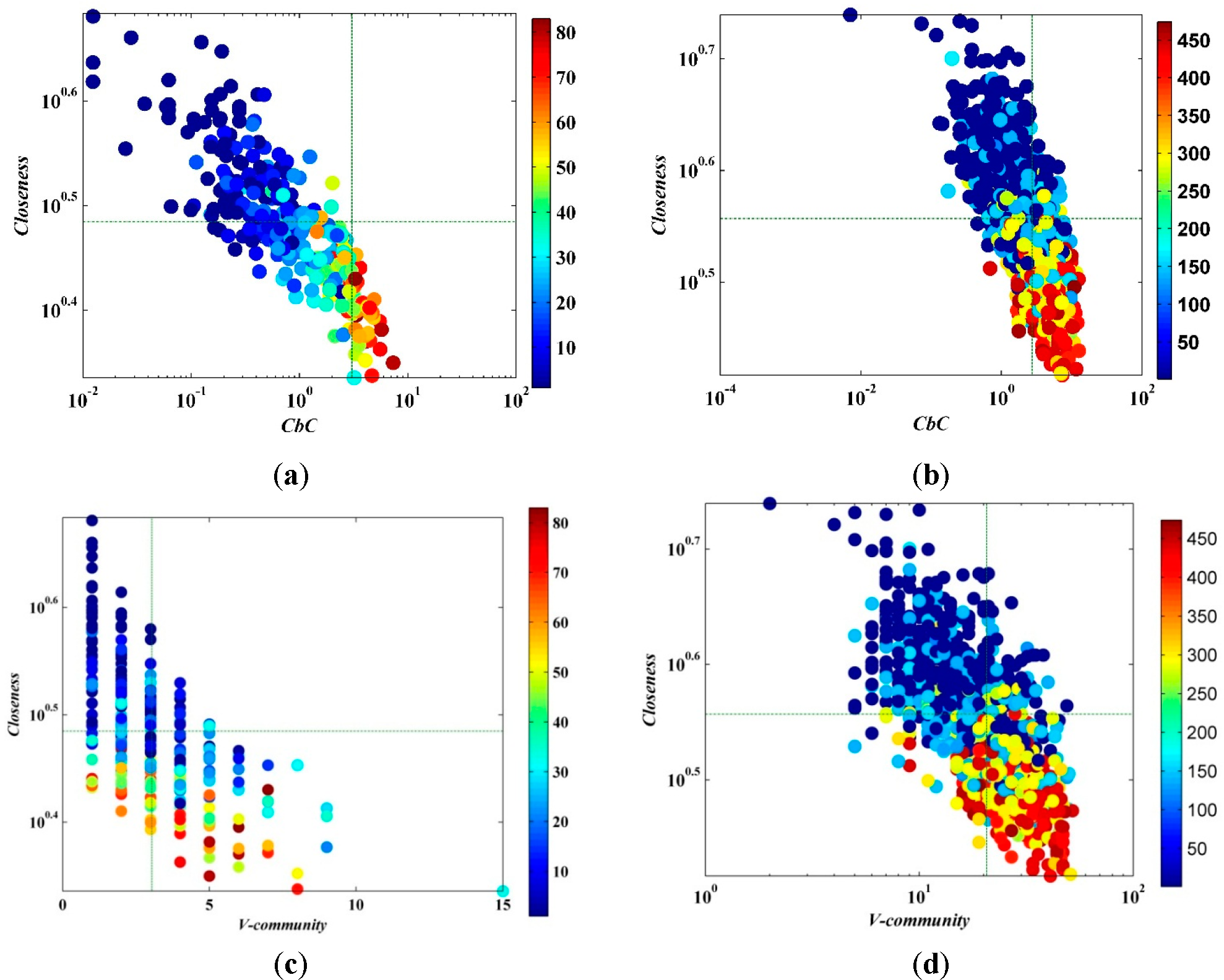
The value of closeness in the manuscript was calculated by Gephi0.8 and the formula was not the reciprocal of the sum on the geodesic distances on all other nodes in the network, but was calculated by the average distance from a given starting node to all other nodes in the network. Consequently, it can be considered as a measure of how long it will take to spread information from a given node to other reachable nodes in the network. The plots of CbC and the closeness of nodes are given in Figure 7; CbC and closeness have a significantly negative correlation. Therefore, the closeness of neighbors with high CbC is far less than for a node with low CbC, i.e., the node with high CbC is mostly situated at the “bridge” of the communities, but it is not located in the central area of the community. It can be seen from the comparison of the spreading capacity of nodes that the node with higher CbC has stronger spreading capability. The same as for betweenness centrality, calculating closeness centrality has a complexity of O(n³).

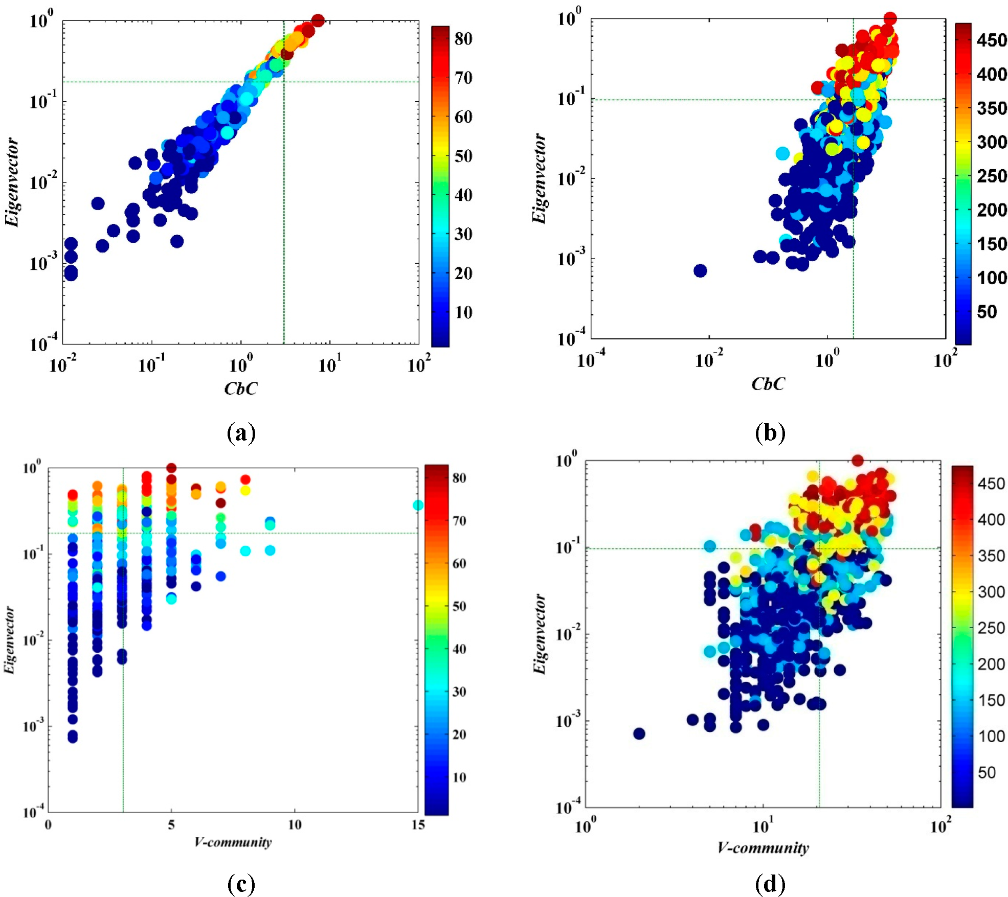
Based on the idea that an actor is more central if it has a relation to actors that are themselves central, it can be argued that the centrality of a node does not only depend on its number of adjacent nodes but also on their value of centrality. For example, Bonacichin [53] defined the centrality of a node as positive multiple of the sum of adjacent centralities. Figure 8 schematizes the correlation between CbC and eigenvector centricity of a node in the network; CbC and eigenvector centricity have significant positive correlation, i.e., the node with higher CbC has larger eigenvector centricity, and vice versa. The computational complexity of eigenvector is O(n²), which is less than betweenness and closeness centrality but still larger than the algorithm we have proposed.

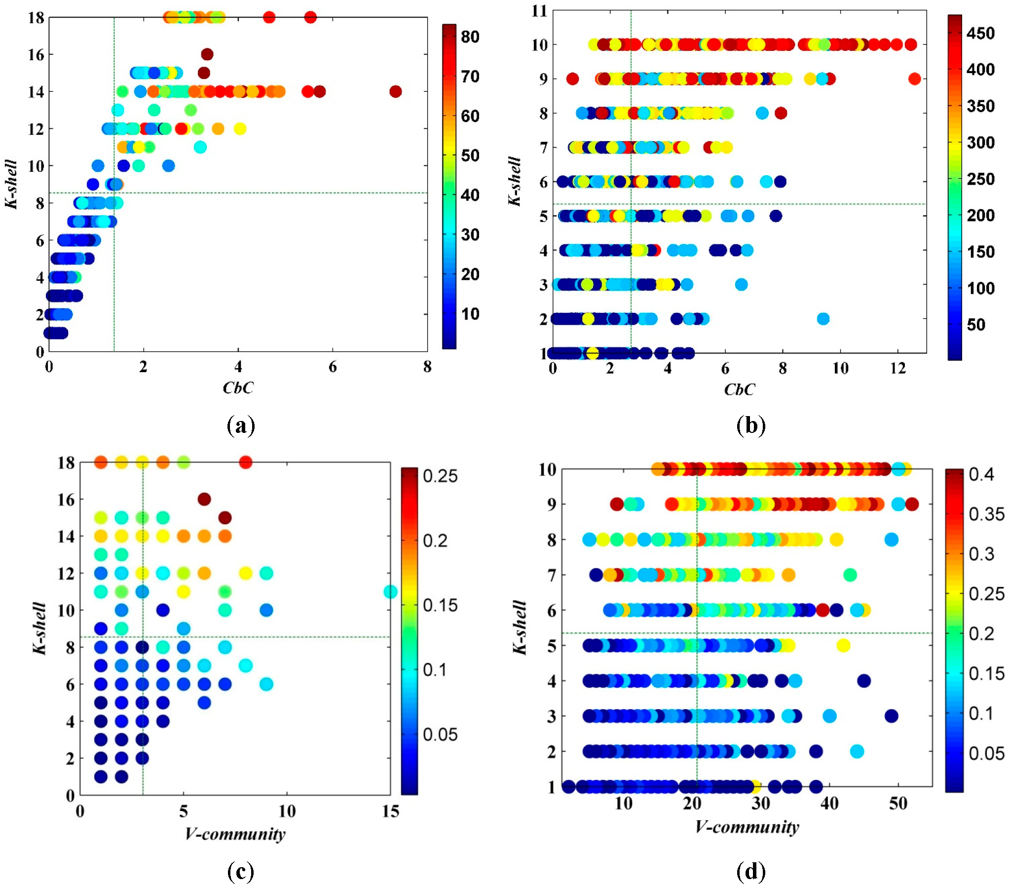
In contrast to common belief, there are plausible circumstances where the best spreaders do not correspond to the most highly connected or the most central people. Thus, [19] suggested that the position of the node relative to the organization of the network determines its spreading influence more than a local property of a node and defined K-shell. The relation between CbC and K-shell value Ks is presented in Figure 9. As Ks in the network is distributed centrally, the positive correlation of CbC and Ks is not very obvious. However, as the Ks values of a large number of nodes in the network are the same, it is deficient to use as an index to measure the importance of nodes. The experiment conducted in this paper will correct to “0.0001” for the CbC of a node. Therefore, it can avoid repetition to the greatest extent. Through the spreading capability of a node, Figure 9 shows that, if the Ks values of the nodes are the same, the node with the higher CbC has the stronger spreading capability.

Furthermore, compared with V-community in Figure 9c,d, the measurement we presented is no longer a discrete variable. Precisely because of the continuity, the ranking of importance can be described by CbC more appropriately in a sense. The details of its advantages will be provided in the next section.

3.3. The Advantage of CbC

Firstly, we compared the Pearson correlation coefficient (r) between spreading capabilities (in the same spreading probability β = 0.05) and CbCs calculated by CNM, Walk Trap and Label Propagation, and further compared the Pearson correlation coefficient (r) between spreading capabilities of nodes and other classical centrality indicators (

Table 7. The Pearson Correlation Coefficient (r) between spreading capabilities and indexes including the classic ones and CbCs calculated by CNM (CbC_CNM), Walk Trap (CbC_WalkTrap) and Label Propagation (CbC_{LabelPropagation}).

Index	Facebook	Metabolic	Email
Degree	0.918997	0.825063	0.913485
Betweenness	0.395862	0.57502	0.748359
Closeness	−0.73634	−0.60029	−0.7392
Eigenvector	0.971692	0.940558	0.951065
Ks	0.867811	0.82172	0.783794
CbCCNM	0.967438	0.840384	0.889797
CbCWalkTrap	0.947099245	0.869187	0.827893
CbCLabelPropagation	0.945307078	0.844415	0.851228

).

By comparing the experimental results in Table 7, the correlations between CbCs and spreading capabilities are all the extremely strong correlations. Furthermore, the results show that the Pearson Correlation Coefficient (r) for CbC is almost larger than that for other centrality measures except the eigenvector. The values of Pearson correlation coefficient on eigenvector centralities are consistently higher than others. Furthermore, in our current research on effects of spreading capability depending on diverse probabilities of propagation, the fascinating results shows that the Pearson correlation coefficient on eigenvector centrality in Email network is declining with the increase of propagation probability. However, the value of the Coefficients are no lower than 0.8, namely, the correlations are all extremely strong ones between eigenvector and those influence ranking results by varying propagation probabilities.

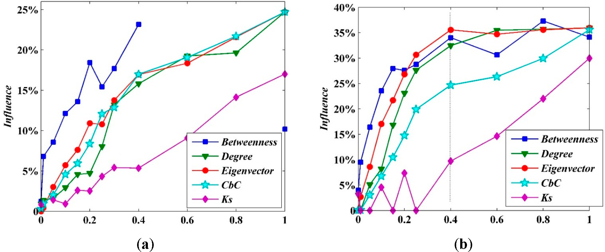
For convenience in computation, one may normalize the variables above by dividing them by N (the number of nodes), and, in doing so, they also have the meaning of “ranking”. The normalization of the indicators (betweenness, degree, eigenvector, CbC and K-shell) is shown in Figure 10. The ordinate axis is the average influence of the infection source. According to the curves, the spreading capability of the sources and the ranking of selected indicators almost have positive correlations. Totally depending on the experimental data results without considering the possible error bars for points, the CbC is the only index that the influence of the source is monotone increasing. Meanwhile, the competitors, degree and eigenvector, both exist in fluctuation; the average influence of larger indexes is lower than that of smaller ones, especially when the indicator has a high level (ranking results of more than 0.4). Nevertheless, the differentials are not significant enough to support such a definitive conclusion, even worse, they are probably caused by possible error. Furthermore, Figure 10b represents that the influence measured by CbC is increasing at a much slower pace. Accordingly, the influence of the source can be ranked by CbC more steadily and homogeneously. Comparing between Figure 10a and Figure 10b, it can be seen clearly that, the larger the network, the more obvious this performance.

In Figure 10, the average influence of sources with level = 0.4 as ranked by CbC is 24%, compared to 35% for those ranked by eigenvector. It is interesting to note that, when the indicators (betweenness and degree) are at a lower level (<0.4), the average influence decreases by approximately 30% to 35%. Some nodes with ordinary index values have distinguished spreading capability. In other words, these “critical influential spreaders” would be neglected by ranking with betweenness, degree or eigenvector. Identifying the influential spreaders, especially these “critical nodes”, is the very advantage of the CbC method.

The influences of the top 1% of nodes are listed in

Table 8. The influence of the top 1% of nodes as ranked by the chosen indicators of the Facebook Network.

Rank	CbC		Degree		Betweenness		Eigenvector		Ks
	ID	Influence	ID	Influence	ID	Influence	ID	Influence	ID	Influence
1	263	0.246914	263	0.246914	186	0.101852	263	0.246914	78	0.231481
2	2	0.246914	78	0.231481	78	0.231481	78	0.231481	33	0.219136
3	78	0.231481	186	0.101852	153	0.064815	2	0.246914	265	0.169753
4	211	0.222222	2	0.246914	33	0.219136	33	0.219136	42	0.145062

(the top four nodes in the Facebook network with 324 nodes) and

Table 9. The influence of the top 1% of nodes as ranked by the chosen indicators of the Email network.

Rank	CbC		Degree		Betweenness		Eigenvector		Ks
	ID	Influence	ID	Influence	ID	Influence	ID	Influence	ID	Influence
1	134	0.350397	105	0.379523	333	0.378641	105	0.379523	389	0.37158
2	205	0.379523	333	0.378641	105	0.379523	16	0.387467	726	0.392763
3	204	0.359223	42	0.377758	23	0.265666	42	0.377758	552	0.383054
4	105	0.379523	23	0.265666	578	0.37158	196	0.27361	299	0.389232
5	219	0.252427	16	0.387467	76	0.383936	333	0.378641	434	0.406002
6	206	0.372462	41	0.38835	233	0.383936	23	0.265666	571	0.262136
7	198	0.416593	196	0.27361	135	0.352162	3	0.381289	788	0.130627
8	196	0.27361	233	0.383936	41	0.38835	41	0.38835	888	0.272727
9	210	0.398941	76	0.383936	355	0.359223	204	0.359223	756	0.37158
10	201	0.377758	21	0.376876	42	0.377758	49	0.227714	887	0.251545
11	140	0.396293	24	0.39188	378	0.35128	21	0.376876	886	0.130627
12	16	0.387467	355	0.359223	429	0.369815	56	0.377758	885	0.139453

(the top 12 nodes in the Email network with 1133 nodes).

Table 8 illustrates that node 211 was identified only by CbC and was neglected by the other indicators. However, the average influence of node 211 is more than 22%, which is much larger than the average value of the entire network (0.077437, as discussed in Section 3.1 above). It is definitely an influential spreader and is 14th when ranked by influential capability. Meanwhile, when ranking by degree or betweenness, node 186 is in the top 1%, but it is in 105th place for influential capability, with only a 10% influential range. Even worse, node 153 is third highest ranking by betweenness but has no more than a 6.5% influential result, even less than the average influence of this network. In addition, the influence of node 33 is marginally lower than that of node 211. Actually, although node 33 is not in the top 1%, it is ranked 8th place by CbC. As expected, with the increase of the network size, the advantages of identifying critical influential spreaders by CbC are more obvious. The results of the Email network are shown in Table 9.

These data depict that nodes 134, 205, 219, 206, 198, 201 and 140 are in the top 1% level ranking by CbC but are ignored by all other indicators. However, the influences of these seven nodes are all significantly greater than the average of the entire network (0.149706), and the influence of node 198 is third highest of all 1133 nodes in the Email network.

Furthermore, as shown in Table 8 and Table 9, the very top 1% nodes ranking by eigenvector centrality, unfortunately, more or less miss some “critical nodes”, which can be explored by CbC. It seems that, although the ranking result by eigenvector centrality of entirety is satisfied, at the top level it is not precise.

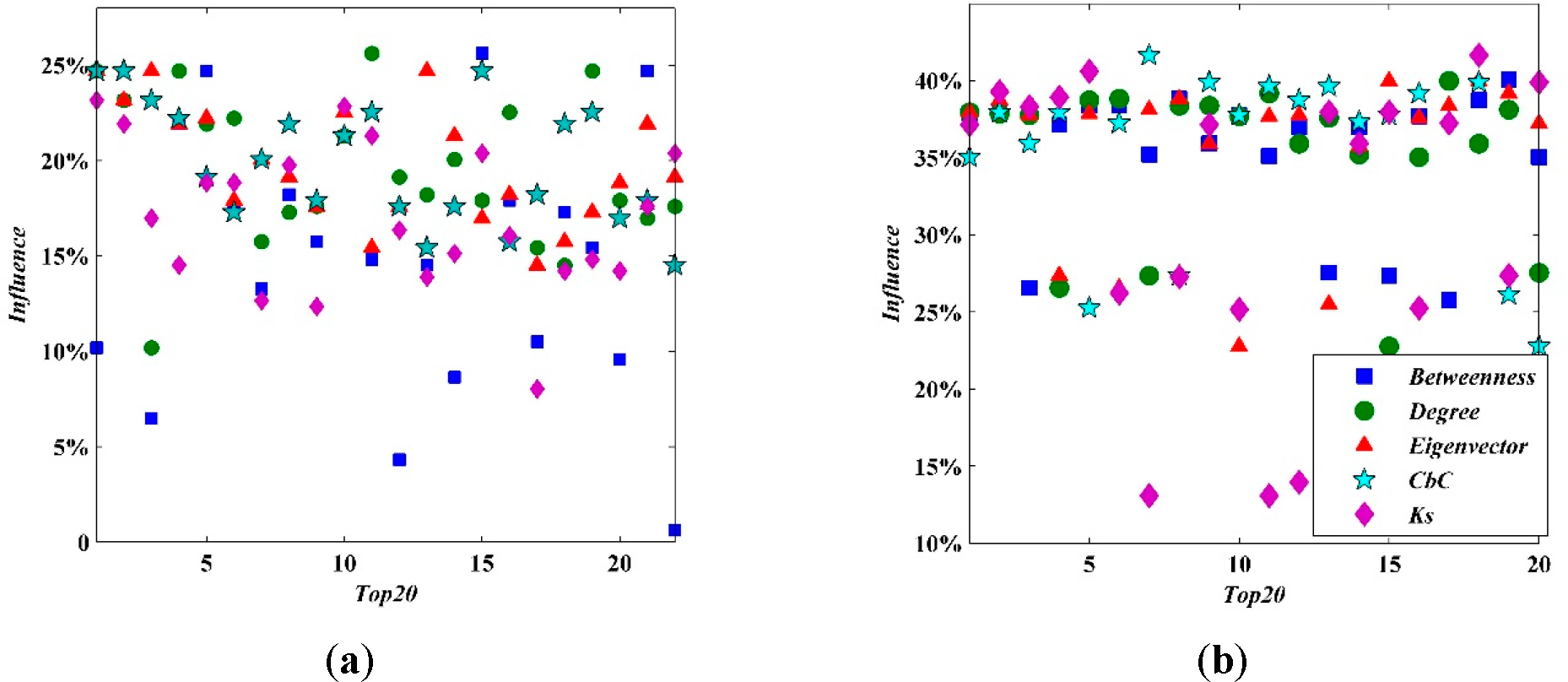
Above all, CbC plays an important role in identifying the critical influential spreaders. However, the influence of source cannot be strictly ranked by any ordered indicators. Given are two scatter diagrams plotting out the influence of the top 20 nodes as ranked by the chosen indicators (Figure 11). Even more, the first and second spreaders are not found by the indicators above. In the Facebook network, the two most influential spreaders are node 16 and node 219 (influences of 0.256173 and 0.253086, respectively). In the Email network, the most influential spreaders are node 396 and node 358 (both have influences of 0.418358). Our research indicates that CbC can help to identify critical spreaders; however, in order to strictly rank these spreaders, further research is needed, which is exactly what we plan to focus on for future work.

4. Stability Analysis of CbC

SIR spreading experiments in different networks are conducted in this chapter. In the Facebook network and Email network, the infection threshold value β should be taken as 0.01~0.10, 0.15, 0.20, 0.25, 0.30, 0.35, 0.40, 0.45 and 0.50. By comparing the infection scale for different infection threshold values in different networks, the stability of the node importance measurement CbC is analyzed.

4.1. The Impact of CbC on the Spreading Influence

First, the average infection rate in the Facebook network when the infection threshold value is 0.03, 0.05, 0.06, 0.10 and 0.50 is investigated (i.e., the arithmetic average of the infection rate obtained from all 324 nodes, which are taken as infection sources, separately, in the network). This is presented in Figure 12 as the curves Facebook0.03, Facebook0.05, Facebook0.06, Facebook0.10 and Facebook0.50.

It can be seen that, with the increase of the infection threshold value β, the average infection rate in the network increases steadily. If a node with higher CbC value is taken as the infection source, the average infection rate of the network is larger until the average infection rate of the network is close to 90%, after which the difference of taking nodes with different CbC values as infection sources is lower. This indicates that, in the Facebook network, the CbC value can be taken as an index to measure the importance of a node, and it is stable enough. The same conclusion remains valid in the Email network. In Figure 12, the curves Email0.05, Email0.10, Email0.25 and Email0.5 are the average infection rates of the Email network when the threshold value is 0.05, 0.10, 0.25 and 0.5, respectively. The spreading capabilities are indicated by the sizes of individuals in Figure 13.

By comparing the curves, Facebook0.05 and Email0.05, Facebook0.10 and Email0.10, and Facebook0.5 and Email0.5, it can be found that the description of node importance by CbC is similar under different networks, and it further proves the stability of using CbC to measure the importance of nodes.

4.2. The Stability of CbC by the Influence Threshold

By comparing the impacts of nodes with different CbC values as infection sources on the entire network using different threshold values in the network, it can be concluded that nodes with higher CbC values as infection sources have a more significant impact on the network. Therefore, CbC value can be used to measure the importance of nodes. Because the CbC values of nodes in the network are different, in order to facilitate comparison, CbC is taken to be an integer in this experiment, and the results are presented in Figure 14.

Figure 14a illustrates that, in the Facebook network, the CbC value interval is 7, namely from 0 to 6, which corresponds to the seven curves in the figure, respectively. Figure 14b illustrates that, in the Email network, the CbC value interval is 13, namely from 0 to 12, which correspond to the 13 curves of the figure, respectively. By contrast, it can be seen that, in the two networks, the node with higher CbC as the infection source has a larger range of network infection, i.e., the node with higher CbC is of greater importance.

5. Conclusions

A node spreading impact measurement method based on CbC structure is proposed in this paper, and the result of key node excavation is compared using traditional measurements (degree, betweenness, closeness, eigenvector and K-shell). Based on the ranking of the importance of existing nodes, the method proposed in this paper can genuinely identify the nodes that are important to the spreading process in the network:

• When other conditions are the same, the node with higher CbC has greater impact on spreading compared with a node with large degree but small CbC.
• CbC can better measure the importance of nodes than betweenness and eigenvector, and its computational complexity is much lower.
• The CbC of a node in the network is correct to 0.0001, thus avoiding repetition to the greatest extent. Therefore, it can avoid causing the same Ks of a large number of nodes in the network like K-shell, which makes it difficult to compare importance. When the Ks values of nodes are the same, the node with a higher CbC value generally has stronger spreading capability.
• With the increase of the infection threshold value, the average infection rate of the network increases stably; when the node with higher CbC is taken as the infection source, the average infection rate of the network is larger until the average infection rate of the network is close to 90%, at which point the difference due to nodes with different I-communities being taken as infection sources is not high. This shows that CbC can be taken as an index to measure the importance of nodes and that it is stable.
• If the node with a higher CbC value is taken as the infection source, the scale of the network infection is larger, i.e., the node with higher CbC value is of greater importance.

References

1. Milgram, S. The small world problem. Psychol. Today. 1967, 1, 60–67. [Google Scholar]
2. Watts, D.J.; Strogatz, S.H. Collective dynamics of ‘small-world’ network. Nature 1998, 393, 440–442. [Google Scholar]
3. Backstrom, L.; Boldi, P.; Rosa, M.; Ugander, J.; Vigna, S. Four degrees of separation 2011, arXiv, 1111.4570v1.
4. Christakis, N.A.; Fowler, J.H. Connected: The Surprising Power of Our Social Networks and How They Shape Our Lives—How Your Friends’ Friends’ Friends Affect Everything You Feel, Think, and Do; Back Bay Books: New York, NY, USA, 2011. [Google Scholar]
5. Barabási, A.-L.; Albert, R. Emergence of scaling in random networks. Science 1999, 286, 509–512. [Google Scholar]
6. Wang, X.-F.; Li, X.; Chen, G.-R. Network Science: An Introduction; Higher Education Press: Beijing, China, 2012; in Chinese. [Google Scholar]
7. Liu, J.-G.; Ren, Z.-M.; Guo, Q.; Wang, B.-H. Node importance ranking of complex networks. Acta Physica Sin. 2013, 62, 178901, in Chinese. [Google Scholar]
8. Albert, R.; Jeong, H.; Barabási, A.-L. Error and attack tolerance of complex networks. Nature 2000, 406, 378–482. [Google Scholar]
9. Pastor-Satorras, R.; Vespignani, A. Epidemic spreading in scale-free networks. Phys. Rev. Lett. 2001, 86, 3200–3203. [Google Scholar]
10. Cohen, R.; Erez, K.; ben-Avraham, D.; Havlin, S. Breakdown of the Internet under intentional attack. Phys. Rev. Lett. 2001, 86, 3682–3685. [Google Scholar]
11. Chen, D.; Lv, L.; Shang, M.; Zhang, Y.; Zhou, T. Identifying influential nodes in complex networks. Physica A 2012, 391, 1777–1787. [Google Scholar]
12. Centola, D. The spread of behavior in an online social network experiment. Science 2010, 329, 1194–1197. [Google Scholar]
13. Ugander, J.; Backstrom, L.; Marlow, C.; Kleinberg, J. Structural diversity in social contagion. Proc. Natl. Acad. Sci. USA 2012, 109, 5962–5966. [Google Scholar]
14. Freeman, L.C. A set of measures of centrality based on betweenness. Sociometry 1977, 40, 35–41. [Google Scholar]
15. Friedkin, N.E. Theoretical foundations for centrality measures. Am. J. Sociol. 1991, 96, 1478–1504. [Google Scholar]
16. Sabidussi, G. The centrality index of a graph. Psyehometrika 1966, 31, 581–603. [Google Scholar]
17. Stephenson, K.; Zelen, M. Rethinking centrality: Methods and examples. Soc. Netw. 1989, 11, 1–37. [Google Scholar]
18. Borgatti, S. Centrality and network flow. Soc. Netw. 2005, 27, 55–71. [Google Scholar]
19. Kitsak, M.; Gallos, L.K.; Havlin, S.; Liljeros, F.; Muchnik, L.; Stanley, H.E.; Makse, H.A. Identifying influential spreaders in complex networks. Nat. Phys. 2010, 6, 888–893. [Google Scholar]
20. Carmi, S.; Havlin, S.; Kirkpatrick, S.; Shavitt, Y.; Shir, E. A model of Internet topology using k-shell decomposition. Proc. Natl. Acad. Sci. USA 2007, 104, 11150–11154. [Google Scholar]
21. Zeng, A.; Zhang, C. Ranking spreaders by decomposing complex networks. Phys. Rev. Lett. 2013, 377, 1031–1035. [Google Scholar]
22. Garas, A.; Schweitzer, F.; Havlin, S. A K-shell decomposition method for weighted networks. New J. Phys. 2012, 14, 083030. [Google Scholar]
23. Liu, J.; Ren, Z.; Guo, Q. Ranking the spreading influence in complex networks. Physica A 2013, 392, 4154–4159. [Google Scholar]
24. Hou, B.; Yao, Y.; Liao, D. Identifying all-around nodes for spreading dynamics in complex networks. Physica A 2012, 391, 4012–4017. [Google Scholar]
25. Kleinberg, J. Authoritative sources in a hyperlinked environment. J. ACM 1999, 46, 604–632. [Google Scholar]
26. Bryan, K.; Leise, T. The $25,000,000,000 eigenvector: The linear algebra behind Google. SIAM Rev. 2006, 48, 569–581. [Google Scholar]
27. Lv, L.; Zhang, Y.; Yeung, C.; Zhou, T. Leaders in social networks, the delicious case. PLoS One 2011, 6, e21202. [Google Scholar]
28. Li, Q.; Zhou, T.; Lu, L.; Chen, D. Identifying influential spreaders by weighted leaderrank. Physica A 2014, 404, 47–55. [Google Scholar]
29. Chen, D.-B.; Gao, H.; Lu, L.; Zhou, T. Identifying influential nodes in large-scale directed networks: The role of clustering. PLoS One 2013, 8, e77455. [Google Scholar]
30. Chen, D.-B.; Xiao, R.; Zeng, A.; Zhang, Y.-C. Path diversity improves the identification of influential spreaders. Europhys. Lett. 2014, 104. [Google Scholar] [CrossRef]
31. Girvan, M.; Newman, M.E.J. Community structure in social and biological networks. Proc. Natl. Acad. Sci. USA 2001, 99, 7821–7826. [Google Scholar]
32. Hu, Q.; Gao, Y.; Ma, P.; Yin, Y.; Zhang, Y.; Xing, C. A New Approach to Identify Influential Spreaders in Complex Networks. In Web-Age Information Management; Lecture Notes in Computer Science, Volume 7923; Springer: Berlin/Heidelberg, Germany, 2013; pp. 99–104. [Google Scholar]
33. Zhao, Z.-Y.; Yu, H.; Zhu, Z.-L.; Wang, X.-F. Identifying influential spreaders based on network community structure. Chin. J. Comput. 2014, 37, 753–766, in Chinese. [Google Scholar]
34. Newman, M.E.J.; Barabási, A.-L.; Watts, D.J. The Structure and Dynamics of Networks; Princeton University Press: New York, NY, USA, 2003. [Google Scholar]
35. Granovetter, M. The strength of weak ties. Am. J. Sociol. 1973, 78, 1360–1380. [Google Scholar]
36. Chen, G.; Wang, X.; Li, X. Introduction to Complex Networks: Models, Structures and Dynamics; Higher Education Press: Beijing, China, 2012. [Google Scholar]
37. Boccaletti, S.; Latora, V.; Moreno, Y.; Chavez, M.; Hwang, D.-U. Complex networks: Structure and dynamics. Phys. Rep. 2006, 424, 175–308. [Google Scholar]
38. Radicchi, F.; Castellano, C.; Cecconi, F.; Loreto, V.; Parisi, D. Defining and identifying communities in networks. Proc. Natl. Acad. Sci. USA 2004, 101, 2658–2663. [Google Scholar]
39. Fortunato, S. Community detection in graphs. Phys. Rep. 2010, 486, 75–174. [Google Scholar]
40. Duch, J.; Arenas, A. Community detection in complex networks using extreme optimization. Phys. Rev. E 2005, 72, 027104. [Google Scholar]
41. Newman, M.E.J.; Girvan, M. Finding and evaluating community structure in networks. Phys. Rev. E 2004, 69, 026113. [Google Scholar]
42. Clauset, A.; Newman, M.E.J.; Moore, C. Finding community structure in very large networks. Phys. Rev. E 2004, 70, 066111. [Google Scholar]
43. Blagus, N.; Šubelj, L.; Bajec, M. Self-similar scaling of density in complex real-world networks. Physica A 2012, 391, 2794–2802. [Google Scholar]
44. Tang, L.; Liu, H. Relational learning via latent social dimensions, Proceedings of the 15th ACM SIGKDD International Conference on Knowledge Discovery and Data Mining, Paris, France, 28 June–1 July 2009; pp. 817–826.
45. Karl, P. Notes on regression and inheritance in the case of two parents. Proc. R. Soc. Lond. 1895, 58, 240–242. [Google Scholar]
46. Pascal, P.; Matthieu, L. Computing communities in large networks using random walks 2005, arXiv, physics/0512106.
47. Blondel, V.D.; Guillaume, J.L.; Lambiotte, R.; Lefebvre, E. Fast unfolding of communities in large networks 2008, arXiv, 0803.0476.
48. Reichardt, J.; Bornholdt, S. Statistical Mechanics of Community Detection. Phys. Rev. E 2006, 74, 016110. [Google Scholar]
49. Traag, V.A.; Bruggeman, J. Community detection in networks with positive and negative links 2008, arXiv, 0811.2329.
50. Raghavan, U.N.; Albert, R.; Kumara, S. Near linear time algorithm to detect community structures in large-scale networks. Phys. Rev. E 2007, 76, 036106. [Google Scholar]
51. Floyd, R.W. Algorithm 97: Shortest path. Commun. ACM 1962, 5, 345–345. [Google Scholar]
52. Brandes, U. A faster algorithm for betweenness centrality. J. Math. Sociol. 2001, 25, 163–177. [Google Scholar]
53. Bonacich, P. Factoring and weighting approaches to status scores and clique identification. J. Math. Sociol. 1972, 2, 113–120. [Google Scholar]
Figure 1. Community structure and CbC indices of a simple network.
Entropy 17 02228f1
Figure 2. Community structure (colors) and CbC (size of individuals) of nodes in the (a) Facebook network, (b) Metabolic network, (c) Email network, (d) Power network, (e) Router network, and (f) Blogcatalog network.
Entropy 17 02228f2
Figure 3. The community structures divided by different algorithms of community detection methods.
Entropy 17 02228f3
Figure 4. Influence capability (size of individuals) of nodes in the (a) Facebook network, (b) Metabolic network, (c) Email network, (d) Power network, (e) Router network, and (f) Blogcatalog network.
Entropy 17 02228f4
Figure 5. The correlation between Degree centrality and CbC in the (a) Facebook network and (b) Email network; compared with V-community in the (c) Facebook network and (d) Email network.
Entropy 17 02228f5
Figure 6. The correlation between Betweenness centrality and CbC in the (a) Facebook network and (b) Email network; compared with V-community in the (c) Facebook network and (d) Email network.
Entropy 17 02228f6
Figure 7. The correlation between Closeness centrality and CbC in the (a) Facebook network and (b) Email network; compared with V-community in the (c) Facebook network and (d) Email network.
Entropy 17 02228f7
Figure 8. The correlation between Eigenvector centrality and CbC in the (a) Facebook network and (b) Email network; compared with V-community in the (c) Facebook network and (d) Email network.
Entropy 17 02228f8
Figure 9. The correlation between K-shell and CbC in the (a) Facebook network and (b) Email network; compared with V-community in the (c) Facebook network and (d) Email network.
Entropy 17 02228f9
Figure 10. The curves of the influence result growing by ranking of the indicators in (a) the Facebook and (b) Email networks.
Entropy 17 02228f10
Figure 11. Plots of the influence results of the top 20 nodes in (a) the Facebook and (b) Email networks.
Entropy 17 02228f11
Figure 12. The Impact of CbC on the Spreading Influence.
Entropy 17 02228f12
Figure 13. The spreading capability of all of the individuals by different infection thresholds β in the Facebook network ((a), (b) and (c)) and Email network ((d), (e) and (f)).
Entropy 17 02228f13
Figure 14. The Stability Analysis of CbC in (a) the Facebook network and (b) Email network.
Entropy 17 02228f14