A Bayesian Decision-Theoretic Approach to Logically-Consistent Hypothesis Testing

Abstract

This work addresses an important issue regarding the performance of simultaneous test procedures: the construction of multiple tests that at the same time are optimal from a statistical perspective and that also yield logically-consistent results that are easy to communicate to practitioners of statistical methods. For instance, if hypothesis A implies hypothesis B, is it possible to create optimal testing procedures that reject A whenever they reject B? Unfortunately, several standard testing procedures fail in having such logical consistency. Although this has been deeply investigated under a frequentist perspective, the literature lacks analyses under a Bayesian paradigm. In this work, we contribute to the discussion by investigating three rational relationships under a Bayesian decision-theoretic standpoint: coherence, invertibility and union consonance. We characterize and illustrate through simple examples optimal Bayes tests that fulfill each of these requisites separately. We also explore how far one can go by putting these requirements together. We show that although fairly intuitive tests satisfy both coherence and invertibility, no Bayesian testing scheme meets the desiderata as a whole, strengthening the understanding that logical consistency cannot be combined with statistical optimality in general. Finally, we associate Bayesian hypothesis testing with Bayes point estimation procedures. We prove the performance of logically-consistent hypothesis testing by means of a Bayes point estimator to be optimal only under very restrictive conditions.

1. Introduction

One could (...) argue that ‘power is not everything’. In particular for multiple test procedures one can formulate additional requirements, such as, for example, that the decision patterns should be logical, conceivable to other persons, and, as far as possible, simple to communicate to non-statisticians.

—G. Hommel and F. Bretz [1]

Multiple hypothesis testing, a formal quantitative method that consists of testing several hypotheses simultaneously [2], has gained considerable ground in the last few decades with the aim of drawing conclusions from data in scientific experiments regarding unknown quantities of interest. Most of the development of multiple hypothesis testing has been focused on the construction of test procedures satisfying statistical optimality criteria, such as the minimization of posterior expected loss functions or the control of various error rates. These advances are detailed, for instance, in [2], [3] (p. 7), [4] and the references therein. However, another important issue concerning multiple hypothesis testing, namely the construction of simultaneous tests that yield coherent results easier to communicate to practitioners of statistical methods, has not been so deeply investigated yet, especially under the Bayesian paradigm. As a matter of fact, most traditional multiple hypothesis testing schemes do not combine statistical optimality with logical consistency. For example, [5] (p. 250) presents a situation regarding the parameter, θ, of a single exponential random variable, X, in which uniformly most powerful (UMP) tests of level 0.05 for the one-sided hypothesis $H_0^{\left(1\right)}:\theta \le 1$ and the two-sided hypothesis $H_0^{\left(2\right)}:\theta \le 1\cup \theta \ge 2$, say ${\phi }_1$ and ${\phi }_2$, respectively, lead to puzzling decisions. In fact, for the sample outcome $X=0.7$, the test ${\phi }_2$ rejects $H_0^{\left(2\right)}$, and because $H_0^{\left(1\right)}$ implies $H_0^{\left(2\right)}$, one may decide to reject $H_0^{\left(1\right)}$, as well. On the other hand, the test ${\phi }_1$ does not reject $H_0^{\left(1\right)}$, a fact that makes a practitioner confused given these conflicting results. In this example, an inconsistency related to nested hypotheses named coherence [6] takes place. Frequently, other logical relationships one may expect from the conclusions drawn from multiple hypothesis testing, such as consonance [6] and compatibility [7], are not met either.

Although several of these properties have been deeply investigated under a frequentist hypothesis-testing framework, Bayesian literature lacks such analyses. In this work, we contribute to this discussion by examining three rational requirements in simultaneous tests under a Bayesian decision-theoretic perspective. In short, we characterize the families of loss functions that induce multiple Bayesian tests that satisfy partially such desiderata. In Section 2, we review and illustrate the concept of a testing scheme (TS), a mathematical object that assigns to each statistical hypothesis of interest a test function. In Section 3, we formalize three consistency relations one may find important to hold in simultaneous tests: coherence, union consonance and invertibility. In Section 4, we provide necessary and sufficient conditions on loss functions to ensure Bayesian tests to meet each desideratum separately, whatsoever the prior distribution for the relevant parameters is. In Section 5, we prove, under quite general conditions, the impossibility of creating multiple tests under a Bayesian decision-theoretic framework that fulfill the triplet of requisites simultaneously with respect to all prior distributions. We also explore the connection between logically-consistent Bayes tests and Bayes point estimation procedures. Final remarks and suggestions for future inquiries are presented in Section 6. All theorems are proven in the Appendix.

2. Testing Schemes

We start by formulating the mathematical setup for multiple Bayesian tests. For the remainder of the manuscript, the parameter space is denoted by Θ and the sample space by $\mathcal{X}$. Furthermore, $\sigma (\Theta )$ and $\sigma \left(\mathcal{X}\right)$ represent σ-fields of subsets of Θ and $\mathcal{X}$, respectively. We consider the Bayesian statistical model $(\mathcal{X}\times \Theta ,\sigma (\mathcal{X}\times \Theta ),\mathrm{I}\mathrm{P})$. The $\mathrm{I}\mathrm{P}$-marginal distribution of θ, namely the prior distribution for θ, is denoted by π, while ${\pi }_x(.)$ represents the posterior distribution for θ given $X=x$, $x\in \mathcal{X}$. Moreover, $P(.|\theta )$ stands for the conditional distribution of the observable X given θ, and $L_x(\theta )$ represents the likelihood function at the point $\theta \in \Theta$ generated by the sample observation $x\in \mathcal{X}$. Finally, let Ψ be the set of all test functions, that is the set of all $\{0,1\}$-valued measurable functions defined on $\mathcal{X}$. As usual, “1” denotes the decision of rejecting the null hypothesis and “0” the decision of not rejecting or accepting it.

Next, we review the definition of a TS, a mathematical device that formally describes the idea that to each hypothesis of interest it is assigned a test function. Although the specification of the hypotheses of interest most of the times depends on the scientific problem under consideration, here, we assume that a decision-maker has to assign a test to each element of $\sigma (\Theta )$. This assumption not only enables us to precisely define the relevant consistency properties, but it also allows multiple Bayesian testing based on posterior probabilities of the hypotheses (a deeper discussion on this issue may be found in [3] (p. 5) and [8]).

Definition 1. (Testing scheme (TS)) Let the σ-field of subsets of the parameter space $\sigma (\Theta )$ be the set of hypotheses to be tested. Moreover, let Ψ be the set of all test functions defined on $\mathcal{X}$. A TS is a function $\phi :\sigma (\Theta )\to \Psi$ that assigns to each hypothesis $A\in \sigma (\Theta )$ the test ${\phi }_A\in \Psi$ for testing A.

Thus, for $A\in \sigma (\Theta )$ and $x\in \mathcal{X}$, ${\phi }_A\left(x\right)=1$ represents the decision of rejecting the hypothesis A when the datum x is observed. Similarly, ${\phi }_A\left(x\right)=0$ represents the decision of not rejecting A. We now present examples of testing schemes.

Example 1. (Tests based on posterior probabilities) Assume $\Theta ={\mathbb{R}}^d$ and $\sigma (\Theta )=\mathcal{B}\left({\mathbb{R}}^d\right)$, the Borelians of ${\mathbb{R}}^d$. Let π be the prior probability distribution for θ. For each $A\in \sigma (\Theta )$, let ${\phi }_A:\mathcal{X}\to \{0,1\}$ be defined by:

$${\phi }_A\left(x\right)=\mathbb{I}\left({\pi }_x\left(A\right)<\frac{1}{2}\right),$$

where ${\pi }_x(.)$ is the posterior distribution of θ, given x. This is the TS that assigns to each hypothesis $A\in \mathcal{B}\left({\mathbb{R}}^d\right)$ the test that rejects it when its posterior probability is smaller than $1/2.$

Recall that, under a Bayesian decision-theoretic perspective, a hypothesis testing for the hypothesis ${\Theta }_0\subseteq \Theta$ [5] (p. 214) is a decision problem in which the action space is $\{0,1\}$ and the loss function $L:\{0,1\}\times \Theta \to \mathbb{R}$ satisfies:

$$\begin{array}{c}\hfill L(1,\theta )\ge L(0,\theta )\text{for}\theta \in {\Theta }_0\text{and}L(1,\theta )\le L(0,\theta )\text{for}\theta \in {\Theta }_0^c,\end{array}$$

(1)

that is, L is such that the wrong decision ought to be assigned a loss at least as large as that assigned to a correct decision (many authors consider strict inequalities in Equation (1)). We call such a loss function a (strict) hypothesis testing loss function.

A solution of this decision problem, named a Bayes test, is a test function ${\phi }^{*}\in \Psi$ derived, for each sample point $x\in \mathcal{X}$, by minimizing the expectation of the loss function L over $\{0,1\}$ with respect to the posterior distribution. That is, for each $x\in \mathcal{X}$,

$$\begin{array}{c}\hfill {\phi }^{*}\left(x\right)=1\iff \mathbb{E}\left[L(1,\theta )\right|X=x]<\mathbb{E}\left[L(0,\theta )\right|X=x],\end{array}$$

where $\mathbb{E}\left[L(d,\theta )\right|X=x]={\int }_{\Theta }L(d,\theta )\mathrm{d}{\pi }_x(\theta )$, $d\in \{0,1\}$. In the case of the equality of the posterior expectations, both zero and one are optimal decisions, and either of them can be chosen as ${\phi }^{*}\left(x\right)$.

When dealing with multiple tests, one can use the above procedure for each hypothesis of interest. Hence, one can derive a Bayes test for each null hypothesis $A\in \sigma (\Theta )$ considering a specified loss function $L_A:\{0,1\}\times \Theta \to \mathbb{R}$ satisfying Equation (1). This is formally described in the following definition.

Definition 2. (TS generated by a family of loss functions) Let $(\mathcal{X}\times \Theta ,\sigma (\mathcal{X}\times \Theta ),\mathrm{I}\mathrm{P})$ be a Bayesian statistical model. Let ${\left(L_A\right)}_{A\in \sigma (\Theta )}$ be a family of hypothesis testing loss functions, where $L_A:\{0,1\}\times \Theta \to \mathbb{R}$ is the loss function for testing $A\in \sigma (\Theta )$. A TS generated by the family of loss functions ${\left(L_A\right)}_{A\in \sigma (\Theta )}$ is any TS φ defined over $\sigma (\Theta )$, such that, $\forall A\in \sigma (\Theta )$, ${\phi }_A$ is a Bayes test for hypothesis A with respect to π considering the loss $L_A$.

The following example illustrates this concept.

Example 2. (Tests based on posterior probabilities) Assume the same scenario as Example 1 and that ${\left(L_A\right)}_{A\in \sigma (\Theta )}$ is a family of loss functions, such that $\forall A\in \sigma (\Theta )$ and $\forall \theta \in \Theta$,

$$L_A(0,\theta )=\mathbb{I}(\theta \notin A)and{L}_A(1,\theta )=\mathbb{I}(\theta \in A),$$

that is, $L_A$ is the 0–1 loss for A ([5] (p. 215)). The testing scheme introduced in Example 1 is a TS generated by the family of 0–1 loss functions.

The next example shows a TS of Bayesian tests motivated by different epistemological considerations (see [9,10] for details), the full Bayesian significance tests (FBST).

Example 3. (FBST testing scheme) Let $\Theta ={\mathbb{R}}^d$, $\sigma (\Theta )=\mathcal{B}\left({\mathbb{R}}^d\right)$ and $f(.)$ be the prior probability density function (pdf) for θ. Suppose that, for each $x\in \mathcal{X}$, there exists $f(.|x)$, the pdf of the posterior distribution of θ, given x. For each hypothesis $A\in \sigma (\Theta )$, let:

$$T_x^A=\left\{\theta \in \Theta :f(\theta |x)>\underset{\theta \in A}{sup}f(\theta |x)\right\}$$

be the set tangent to the null hypothesis, and let $e{v}_x\left(A\right)=1-{\pi }_x\left(T_x^A\right)$ be the Pereira–Stern evidence value for A (see [11] for a geometric motivation). One can define a TS φ by:

$${\phi }_A\left(x\right)=\mathbb{I}\left(e{v}_x\left(A\right)\le c\right),\forall A\in \sigma (\Theta ) and \forall x\in \mathcal{X},$$

in which $c\in [0,1]$ is fixed. In other words, one does not reject the null hypothesis when its evidence is larger than c.

We end this section by defining a TS generated by a point estimation procedure, an intuitive concept that plays an important role in characterizing logically-consistent simultaneous tests.

Definition 3. (TS generated by a point estimation procedure) Let $\delta :\mathcal{X}⟶\Theta$ be a point estimator for θ ([5] (p. 296)). The TS generated by δ is defined by:

$${\phi }_A\left(x\right)=\mathbb{I}(\delta \left(x\right)\notin A).$$

Hence, the TS generated by the point estimator δ rejects hypothesis A after observing x if, and only if, the point estimate for θ, $\delta \left(x\right)$, is not in A.

Example 4. (TS generated by a point estimation procedure) Let $\Theta =\mathbb{R}$, $\sigma (\Theta )=\mathcal{P}(\Theta )$ and $X_1\dots ,X_n|\theta$ i.i.d. $N(\theta ,1)$. The TS generated by the sample mean, X, rejects $A\in \sigma (\Theta )$ when x is observed if $x\notin A$.

3. The Desiderata

In this section, we review three properties one may expect from simultaneous test procedures: coherence, invertibility and union consonance.

3.1. Coherence

When a hypothesis is tested by a significance test and is not rejected, it is generally agreed that all hypotheses implied by that hypothesis (its “components”) must also be considered as non-rejected.

—K. R. Gabriel [6]

The first property concerns nested hypotheses and was originally defined by [6]. It states that if hypothesis $H_0^{\left(1\right)}$ implies hypothesis $H_0^{\left(2\right)}$, that is $H_0^{\left(1\right)}\subseteq H_0^{\left(2\right)}$, then the rejection of $H_0^{\left(2\right)}$ implies the rejection of $H_0^{\left(1\right)}$. In the context of TSs, we have the following definition.

Definition 4. (Coherence) A testing scheme φ is coherent if:

$$\forall A, B\in \sigma (\Theta ), A\subseteq B\Rightarrow {\phi }_A\ge {\phi }_B, i.e., \forall x\in \mathcal{X}, {\phi }_A\left(x\right)\ge {\phi }_B\left(x\right).$$

In other words, if after observing x, a hypothesis is rejected, any hypothesis that implies it has to be rejected, as well.

The testing schemes introduced in Examples 1, 3 and 4 are coherent. Indeed, in Example 1, coherence is a consequence of the monotonicity of probability measures, while in Example 3, it follows from the fact that if $A\subseteq B$, then $T_x^B\subseteq T_x^A$ and, therefore, $e{v}_x\left(A\right)\le e{v}_x\left(B\right)$. In Example 4, coherence is immediate. On the other hand, testing schemes based on UMP tests or generalized likelihood ratio tests with a common fixed level of significance are not coherent in general. Neither are TSs generated by some families of loss functions (see Section 4). Next, we illustrate that even test procedures based on p-values or Bayes factors may be incoherent.

Example 5. Suppose that in a case-control study, one measures the genotype in a certain locus for each individual of a sample. Results are shown in Table 1. These numbers were taken from a study presented by [12] that had the aim of verifying the hypothesis that subunits of the gene $GAB{A}_A$ contribute to a condition known as methamphetamine use disorder. Here, the set of all possible genotypes is $\mathbb{G}=\{AA,AB,BB\}.$ Let $\gamma =({\gamma }_{AA},{\gamma }_{AB},{\gamma }_{BB})$, where ${\gamma }_i$ is the probability that an individual from the case group has genotype i. Similarly, let $\pi =({\pi }_{AA},{\pi }_{AB},{\pi }_{BB})$, where ${\pi }_i$ is the probability that an individual of control group has genotype i.

In this context, two hypotheses are of interest: the hypothesis that the genotypic proportions are the same in both groups, $H_0^G:\gamma =\pi$, and the hypothesis that the allelic proportions are the same in both groups $H_0^A:{\gamma }_{AA}+\frac{1}{2}{\gamma }_{AB}={\pi }_{AA}+\frac{1}{2}{\pi }_{AB}$. The p-values obtained using chi-square tests for these hypotheses are, respectively, 0.152 and 0.069. Hence, at the level of significance $\alpha =10\%$, the TS given by chi-square tests rejects $H_0^A$, but does not reject $H_0^G$. That is, the TS leads a practitioner to believe that the allelic proportions are different in both groups, but it does not suggest any difference between the genotypic proportions. This is absurd!If the allelic proportions are not the same in both groups, the genotypic proportions cannot be the same either. Indeed, if the latter were the same, then ${\gamma }_i={\pi }_i$, $\forall i\in \mathbb{G}$, and hence, $\theta \in H_0^A$. This example is further discussed in [8,13].

Table 1. Genotypic sample frequencies.

	AA	AB	BB	Total
Case	55	83	50	188
Control	24	42	39	105

Table 1. Genotypic sample frequencies.

	AA	AB	BB	Total
Case	55	83	50	188
Control	24	42	39	105

Several other (in)coherent testing schemes are explored by [8,14].

Coherence is by far the most emphasized logical requisite for simultaneous test procedures in the literature. It is often regarded as a sensible property by both theorists and practitioners of statistical methods who perceive a hypothesis test as a two-fold (accept/reject) decision problem. On the other hand, adherents to evidence-based approaches to hypothesis testing [15] do not see the need for coherence. Under the frequentist approach to hypothesis testing, the construction of coherent procedures is closely associated with the so-called closure methods [16,17]. Many results on coherent classical tests are shown in [6,17], among others. On the other hand, coherence has not been deeply investigated from a Bayesian standpoint yet, except for [18], who relate coherence with admissibility and Bayesian optimality in certain situations of finitely many hypotheses of interest. In Section 4, we provide a characterization of coherent testing schemes under a decision-theoretic framework.

3.2. Invertibility

There is a duality between hypotheses and alternatives which is not respected in most of the classical hypothesis-testing literature. (...) suppose that we decide to switch the names of alternative and hypothesis, so that ${\Omega }_H$ becomes ${\Omega }_A$, and vice versa. Then we can switch tests from ϕ to $\psi =1-\varphi$ and the “actions” accept and reject become switched.

—M. J. Schervish [5] (p. 216)

The duality mentioned in the quotation above is formally described in the next definition.

Definition 5. (Invertibility) A testing scheme φ satisfies invertibility if:

$$\forall A\in \sigma (\Theta ), {\phi }_{A^c}=1-{\phi }_A.$$

In other words, it is irrelevant to decision-making which hypothesis is labeled as null and which is labeled as alternative.

Unlike coherence, there is no consensus among statisticians on how reasonable invertibility is. While it is supported by many decision-theorists, invertibility is usually discredited by advocates of the frequentist theory owing to the difference between the interpretations of “not reject a hypothesis” and “accept a hypothesis” under various epistemological viewpoints (the reader is referred to [7] for a discussion on this distinction). As a matter of fact, invertibility can also be seen, from a logic perspective, as a version of the law of the excluded middle, which itself represents a gap between schools of logic ([19] (p. 32)). In spite of the controversies on invertibility, it seems to be beyond any argument the fact that the absence of invertibility in multiple tests may lead a decision-maker to be puzzled by senseless conclusions, such as the simultaneous rejections of both a hypothesis and its alternative. The following example illustrates this point.

Example 6. Suppose that $X|\theta \sim Normal(\theta ,1)$, and consider that the parameter space is $\Theta =\{-3,3\}$. Assume one wants to test the following null hypotheses:

$$\begin{array}{c}\hfill H_0^A:\theta =3and{H}_0^B:\theta =-3\end{array}$$

The Neyman–Pearson tests for these hypotheses have the following critical regions, at the level 5%, respectively:

$$\{x\in \mathbb{R}:x<1.35\}and\{x\in \mathbb{R}:x>-1.35\}.$$

Hence, if we observe $x=-0.5$, we reject both $H_0^A$ and $H_0^B$, even though $H_0^A\cup H_0^B=\Theta$! 

The testing schemes of Examples 2 and 4 satisfy invertibility. In Example 4, it is straightforward to verify this. In Example 2, it follows essentially from the equivalence ${\pi }_x\left(A\right)<1/2\iff {\pi }_x\left(A^c\right)>1/2$. If ${\pi }_x\left(A\right)\ne 1/2$ for each sample x and for all $A\in \sigma (\Theta )$, the unique TS generated by the 0–1 loss functions satisfies invertibility. Otherwise, there is a testing scheme generated by such losses that is still in line with this property. Indeed, for any $A\in \sigma (\Theta )$ and $x_0\in \mathcal{X}$, such that ${\pi }_{x_0}\left(A\right)=1/2$, the decision of rejecting A (not rejecting $A^c$) after observing $x_0$ has the same expected loss as the decision of not rejecting (rejecting) it. Thus, among all testing schemes generated by the 0–1 loss functions, which are all equivalent from a decision-theoretic point of view ([20] (p. 123)), a decision-maker can always choose a TS ${\phi }^{\prime }$, such that ${\phi }_{A^c}^{\prime }\left(x_0\right)=1-{\phi }_A^{\prime }\left(x_0\right)$ for all $A\in \sigma (\Theta )$, and $x_0\in \mathcal{X}$, such that ${\pi }_{x_0}\left(A\right)=1/2$. Such a TS ${\phi }^{\prime }$ meets invertibility.

3.3. Consonance

... a test for ${\left({\cup }_{i\in I}{H}_i\right)}^c$ versus $\left({\cup }_{i\in I}{H}_i\right)$ may result in rejection which then indicates that at least one of the hypotheses $H_i$, $i\in I$, may be true.

—H. Finner and K. Strassburger [21]

The third property concerns two hypotheses, say A and B, and their union, $A\cup B$. It is motivated by the fact that in many cases, it seems reasonable that a testing scheme that retains the union of these hypotheses should also retain at least one of them. This idea is generalized in Definition 6.

Definition 6. (Union Consonance) A TS φ satisfies the finite (countable) union consonance if for all finite (countable) set of indices I,

$$\forall {\left\{A_i\right\}}_{i\in I}\subseteq \sigma (\Theta ),{\phi }_{{\cup }_{i\in I}{A}_i}\ge min{\left\{{\phi }_{A_i}\right\}}_{i\in I}.$$

In other words, if we retain the union of the hypotheses ${\cup }_{i\in I}{A}_i$, we should not reject at least one of the $A_i$’s.

There are several testing schemes that meet union consonance. For instance, TSs generated by point estimation procedures, TSs of Aitchison’s confidence-region tests [22] and FBST TSs (under quite general conditions; see [8]) satisfy both finite and countable union consonance.

Although union consonance may not be considered as appealing as coherence for simultaneous test procedures, it was hinted at in a few relevant works. For instance, the interpretation given by [21] on the final joint decisions derived from partial decisions implicitly suggests that union consonance is reasonable: they suggest one should consider $B:={\cup }_{A:{\phi }_A\left(x\right)=1}A$ to be the set of all parameter values rejected by the simultaneous procedure at hand when x is observed. Under this reading, it seems natural to expect that ${\phi }_B\left(x\right)=1$, which is exactly what the union consonance principle states. As a matter of fact, the general partitioning principle proposed by these authors satisfies union consonance. It should also be mentioned that union consonance, together with coherence, plays a key role in the possibilistic abstract belief calculus [23]. In addition, an evidence-based approach detailed in [24] satisfies both consonance and invertibility.

We end this section by stating a result derived from putting these logical requirements together.

Theorem 1. Let Θ be a countable parameter space and $\sigma (\Theta )=\mathcal{P}(\Theta )$. Let φ be a testing scheme defined on $\sigma (\Theta )$. The TS φ satisfies coherence, invertibility and countable union consonance if, and only if, there is a point estimator $\delta :\mathcal{X}\to \Theta$, such that φ is generated by δ.

Theorem 1 is also valid for finite union consonance with the obvious adaptation.

4. A Bayesian Look at Each Desideratum

In the previous section, we provided several examples of testing schemes satisfying some of the logical properties reviewed therein. In particular, a testing scheme generated by the family of 0–1 loss functions (Example 2) was shown to fulfill both coherence and invertibility. However, not all families of loss functions generate a TS meeting any of these requisites, as is shown in the examples below.

Example 7. Suppose that $X|\theta \sim Bernoulli(\theta )$ and that one is interested in testing the null hypotheses:

$$H_0^A:\theta \le 0.4and{H}_0^B:\theta \le 0.5.$$

Furthermore, assume $\theta \sim Uniform(0,1)$ a priori and that he uses the loss functions from Table 2 to perform the tests.

Thus, Bayes tests for testing $H_0^A$ and $H_0^B$ are, respectively,

$${\phi }_A\left(x\right)=\mathbb{I}\left(\mathrm{I}\mathrm{P}(\theta \le 0.4|x)\le 1/7\right)and{\phi }_B\left(x\right)=\mathbb{I}\left(\mathrm{I}\mathrm{P}(\theta \le 0.5|x)\le 1/3\right).$$

As $\theta |x\sim Beta(2,1)$ if $x=1$ is observed, then $\mathrm{I}\mathrm{P}(\theta \le 0.4|x)=0.16$ and $\mathrm{I}\mathrm{P}(\theta \le 0.5|x)=0.25$, so that one does not reject $H_0^A$, but rejects $H_0^B$. Since $H_0^A\subset H_0^B$, we conclude that coherence does not hold.

Table 2. Loss functions for tests of Example 7.

	State of Nature
Decision	$\theta \in H_0^A$	$\theta \notin H_0^A$
0	0	1
1	6	0

	State of Nature
Decision	$\theta \in H_0^A$	$\theta \notin H_0^A$
0	0	1
1	6	0

	State of Nature
Decision	$\theta \in H_0^B$	$\theta \notin H_0^B$
0	0	1
1	2	0

	State of Nature
Decision	$\theta \in H_0^B$	$\theta \notin H_0^B$
0	0	1
1	2	0

Intuitively, incoherence takes place because the loss of falsely rejecting $H_0^A$ is three-times as large as the loss of falsely rejecting $H_0^B$, while the corresponding errors of Type II are of the same magnitude. Hence, these loss functions reveal that the decision-maker is more reluctant to reject $H_0^A$ than to reject $H_0^B$ in such a way that he only needs little evidence to accept $H_0^A$ (posterior probability greater than 1/7) when compared to the amount of evidence needed to accept $H_0^B$ (posterior probability greater than 1/3). Thus, it is not surprising at all that in this case, the tests do not cohere for some priors.

Example 8. In the setup of Example 7, suppose one also needs to test the null hypothesis $H_0^{B^c}:\theta >0.5$ by taking into account the loss function in Table 3.

The Bayes test for $H_0^{B^c}$ is then to reject it if $\mathrm{I}\mathrm{P}(\theta >0.5|x)<4/5$. For $x=1$, $\mathrm{I}\mathrm{P}(\theta >0.5|x)=0.75$, and consequently, $H_0^{B^c}$ is rejected. As both $H_0^B$ and $H_0^{B^c}$ are rejected when $x=1$ is observed, these tests do not satisfy invertibility.

Table 3. Loss function for Example 8.

	State of Nature
Decision	$\theta \in H_0^{B^c}$	$\theta \notin H_0^{B^c}$
0	0	4
1	1	0

Table 3. Loss function for Example 8.

	State of Nature
Decision	$\theta \in H_0^{B^c}$	$\theta \notin H_0^{B^c}$
0	0	4
1	1	0

The absence of invertibility is somewhat expected here, because the degree to which the decision-maker believes an incorrect decision of choosing $H_0^B$ to be more serious than an incorrect decision of choosing $H_0^{B^c}$ is not the same whether $H_0^B$ is regarded as the “null” or the “alternative” hypothesis. More precisely, while the decision-maker assigns a loss to the error of Type I that is the double of the one assigned to the error of Type II when testing the null hypothesis $H_0^B$, he evaluates the loss of falsely accepting $H_0^{B^c}$ to be four-times (not twice!) as large as that of falsely rejecting it when $H_0^{B^c}$ is the null hypothesis.

The examples we have examined so far give rise to the question: from a decision-theoretic perspective, what conditions must be imposed on a family of loss functions so that the resultant Bayesian testing scheme meets coherence (invertibility)? Next, we offer a solution to this question. We first give a definition in order to simplify the statement of the main results of this section.

Definition 7. (Relative loss) Let $L_A$ be a loss function for testing the hypothesis $A\in \sigma (\Theta )$. The function ${\Delta }_A:\Theta \to \mathbb{R}$ defined by:

$${\Delta }_A(\theta )=\left\{\begin{array}{cc}{L}_A(1,\theta )-L_A(0,\theta ),\hfill & \mathrm{if} \theta \in A\hfill \\ L_A(0,\theta )-L_A(1,\theta ),\hfill & \mathrm{if} \theta \notin A\hfill \end{array}\right.$$

is named the relative loss of $L_A$ for testing A.

In short, the relative loss measures the difference between losses of taking the wrong and the correct decisions. Thus, the relative loss of any hypothesis testing loss function is always non-negative.

A careful examination of Example 7 hints that in order to obtain coherent tests, the “larger” (the “smaller”) the null hypothesis of interest is, the more cautious about falsely rejecting (accepting) it the decision-maker ought to be. This can be quantified as follows: for hypotheses A and B, such that $A\subseteq B$ and with corresponding hypothesis testing loss functions $L_A$ and $L_B$, if ${\theta }_1\in A$, then ${\Delta }_B\left({\theta }_1\right)$ should be at least as large as ${\Delta }_A\left({\theta }_1\right)$. Similarly, if ${\theta }_2\in B^c$, then ${\Delta }_B\left({\theta }_2\right)$ should be at most ${\Delta }_A\left({\theta }_2\right)$. 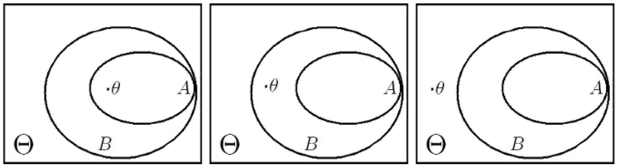Such conditions are also appealing, since it seems reasonable that greater relative losses should be assigned to greater “distances” between the parameter and the wrong decision. For instance, if $\theta \in A$ (and consequently, $\theta \in B$), the rougher error of rejecting B should be penalized more heavily than the error of rejecting A; Figure 1 enlightens this idea.

Figure 1. Interpretation of sensible relative losses: rougher errors of decisions should be assigned larger relative losses.

Figure 1. Interpretation of sensible relative losses: rougher errors of decisions should be assigned larger relative losses.

These conditions, namely:

$${\Delta }_A\left({\theta }_1\right)\le {\Delta }_B\left({\theta }_1\right),\forall {\theta }_1\in A\text{and}{\Delta }_A\left({\theta }_2\right)\ge {\Delta }_B\left({\theta }_2\right),\forall {\theta }_2\in B^c,$$

are sufficient for coherence. As a matter of fact, Theorem 2 states that the weaker condition:

$${\Delta }_A\left({\theta }_1\right){\Delta }_B\left({\theta }_2\right)\le {\Delta }_A\left({\theta }_2\right){\Delta }_B\left({\theta }_1\right),\forall {\theta }_1\in A,\forall {\theta }_2\in B^c,$$

is necessary and sufficient for a family of hypothesis testing loss functions to induce a coherent testing scheme with respect to each prior distribution for θ. Henceforward, we assume that $\mathbb{E}\left(L_A(d,\theta )\right|x)<\infty$, for all $A\in \sigma (\Theta )$, $d\in \{0,1\}$ and $x\in \mathcal{X}$.

Theorem 2. Let ${\left(L_A\right)}_{A\in \sigma (\Theta )}$ be a family of hypothesis testing loss functions. Suppose that for all ${\theta }_1,{\theta }_2\in \Theta$, there is $x\in \mathcal{X}$, such that $L_x\left({\theta }_1\right),L_x\left({\theta }_2\right)>0$. Then, for all prior distributions π for θ, there exists a testing scheme generated by ${\left(L_A\right)}_{A\in \sigma (\Theta )}$ with respect to π that is coherent if, and only if, ${\left(L_A\right)}_{A\in \sigma (\Theta )}$ is such that for all $A,B\in \sigma (\Theta )$ with $A\subseteq B$:

$$\begin{array}{c}\hfill {\Delta }_A\left({\theta }_1\right){\Delta }_B\left({\theta }_2\right)\le {\Delta }_A\left({\theta }_2\right){\Delta }_B\left({\theta }_1\right),\forall {\theta }_1\in A,\forall {\theta }_2\in B^c.\end{array}$$

(2)

Notice that the “if” part of Theorem 2 still holds for families of hypothesis testing loss functions that depend also on the sample. Theorem 2 characterizes, under certain conditions, all families of loss functions that induce coherent tests, no matter what the decision-maker’s opinion (prior) on the unknown parameter is. Although the result of Theorem 2 is not properly normative, any Bayesian decision-maker can make use of it to prevent himself from drawing incoherent conclusions from multiple hypothesis testing by checking whether his personal losses satisfy the condition in Equation (2).

Many simple families of loss functions generate coherent tests, as we illustrate in Examples 9 and 10.

Example 9. Consider, for each $A\in \sigma (\Theta )$, the loss function $L_A$ in Table 4 to test the null hypothesis A, in which $\lambda :\sigma (\Theta )\to {\mathbb{R}}_{+}$ is any finite measure, such that $\lambda (\Theta )>0$. This family of loss functions satisfies the condition in Equation (2) for coherence as for all $A,B\in \sigma (\Theta )$, such that $A\subseteq B$, and for all ${\theta }_1\in A$ and ${\theta }_2\in B^c$, ${\Delta }_A\left({\theta }_1\right)=\lambda \left(A\right)$, ${\Delta }_B\left({\theta }_2\right)=\lambda \left(B^c\right)$, ${\Delta }_A\left({\theta }_2\right)=\lambda \left(A^c\right)$ and ${\Delta }_B\left({\theta }_1\right)=\lambda \left(B\right)$.

Table 4. Loss function $L_A$ for testing A.

	State of Nature
Decision	$\theta \in A$	$\theta \notin A$
0	0	$\lambda \left(A^c\right)$
1	$\lambda \left(A\right)$	0

Table 4. Loss function $L_A$ for testing A.

	State of Nature
Decision	$\theta \in A$	$\theta \notin A$
0	0	$\lambda \left(A^c\right)$
1	$\lambda \left(A\right)$	0

As a matter of fact, if for each $A\in \sigma (\Theta )$, $L_A$ is a $0-1-c_A$ loss function ([5] (p. 215)), with $0<c_A\le c_B$ if $A\subseteq B$, then the family ${\left(L_A\right)}_{A\in \sigma (\Theta )}$ will induce a coherent TS for each prior for θ.

Example 10. Assume Θ is equipped with a distance, say d. Define, for each $A\in \sigma (\Theta )$ the loss function $L_A$ for testing A by:

$$L_A(0,\theta )=d^{*}(\theta ,A)\text{and}{L}_A(1,\theta )=d^{*}(\theta ,A^c),$$

where $d^{*}(\theta ,A)={inf}_{a\in A}d(\theta ,a)$ is the distance between $\theta \in \Theta$ and A. For $A,B\in \sigma (\Theta )$, such that $A\subseteq B$, and for ${\theta }_1\in A$ and ${\theta }_2\in B^c$, ${\Delta }_A\left({\theta }_1\right)=d^{*}({\theta }_1,A^c)$, ${\Delta }_B\left({\theta }_2\right)=d^{*}({\theta }_2,B)$, ${\Delta }_A\left({\theta }_2\right)=d^{*}({\theta }_2,A)$ and ${\Delta }_B\left({\theta }_1\right)=d^{*}({\theta }_1,B^c)$. These values satisfy Equation (2) from Theorem 2. Hence, families of loss functions based on distances as the above generate Bayesian coherent tests.

Next, we characterize Bayesian tests with respect to invertibility. In order to obtain TSs that meet invertibility, it seems reasonable that when the null and alternative hypotheses are switched, the relative losses ought to remain the same. That is to say, when testing the null hypothesis A, the relative loss at each point $\theta \in \Theta$, ${\Delta }_A(\theta )$, should be equal to the relative loss ${\Delta }_{A^c}(\theta )$ when $A^c$ is the null hypothesis instead. This condition is sufficient, but not necessary for a family of loss functions to induce tests fulfilling this logical requisite with respect to all prior distributions. In Theorem 3, however, we provide necessary and sufficient conditions for invertibility.

Theorem 3. Let ${\left(L_A\right)}_{A\in \sigma (\Theta )}$ be a family of hypothesis testing loss functions. Suppose that for all ${\theta }_1,{\theta }_2\in \Theta$, there is $x\in \mathcal{X}$, such that $L_x\left({\theta }_1\right),L_x\left({\theta }_2\right)>0$. Then, for all prior distributions π for θ, there exists a testing scheme generated by ${\left(L_A\right)}_{A\in \sigma (\Theta )}$ with respect to π that satisfies invertibility if, and only if, ${\left(L_A\right)}_{A\in \sigma (\Theta )}$ is such that for all $A\in \sigma (\Theta )$:

$$\begin{array}{c}\hfill {\Delta }_A\left({\theta }_1\right){\Delta }_{A^c}\left({\theta }_2\right)={\Delta }_{A^c}\left({\theta }_1\right){\Delta }_A\left({\theta }_2\right),\forall {\theta }_1\in A{\theta }_2\in A^c.\end{array}$$

(3)

Condition Equation (3) is equivalent (for strict hypothesis testing loss functions) to impose, for each $A\in \sigma (\Theta )$, that the function $\frac{{\Delta }_A(.)}{{\Delta }_{A^c}(.)}$ to be constant over Θ. We should mention that the “if” part of Theorem 3 still holds for hypothesis testing loss functions satisfying (Equation (3)) that also depend on the sample x.

The families of loss functions introduced in Examples 9 and 10 satisfy (Equation (3)). Thus, such families of losses ensure the construction of simultaneous Bayes tests that are in conformity with both coherence and invertibility for all prior distributions on $\sigma (\Theta )$. Thus, if one believes these (two) logical requirements to be of primary importance in multiple hypothesis testing, he can make use of any of these families of loss functions to perform tests satisfactorily. Other simple loss functions also lead to TSs that meet invertibility: for instance, any family of 0–1–c loss functions for which $c_{A^c}=1/c_A$ for all $A\in \sigma (\Theta )$ leads to invertible TSs.

We end this section by examining union consonance under a decision-theoretic point of view. From Definition 6, it appears that a necessary condition for the derivation of consonant tests is that “smaller” (“larger”) null hypotheses ought to be assigned greater losses for false rejection (acceptance). More precisely, for $A,B\in \sigma (\Theta )$, if ${\theta }_1\in A\cup B$, then it seems that either ${\Delta }_{A\cup B}\left({\theta }_1\right)\le {\Delta }_A\left({\theta }_1\right)$ or ${\Delta }_{A\cup B}\left({\theta }_1\right)\le {\Delta }_B\left({\theta }_1\right)$ should hold. If ${\theta }_2\in {(A\cup B)}^c$, then it is reasonable that either ${\Delta }_{A\cup B}\left({\theta }_2\right)\ge {\Delta }_A\left({\theta }_2\right)$ or ${\Delta }_{A\cup B}\left({\theta }_2\right)\ge {\Delta }_B\left({\theta }_2\right)$. The next theorem shows that this is nearly the case. However, it is still unknown whether sufficient conditions for union consonance are determinable.

Theorem 4. Let ${\left(L_A\right)}_{A\in \sigma (\Theta )}$ be a family of hypothesis testing loss functions. Suppose that for all ${\theta }_1,{\theta }_2\in \Theta$, there is $x\in \mathcal{X}$, such that $L_x\left({\theta }_1\right),L_x\left({\theta }_2\right)>0$. If for all prior distribution π for θ, there exists a testing scheme generated by ${\left(L_A\right)}_{A\in \sigma (\Theta )}$ with respect to π that satisfies finite union consonance, then ${\left(L_A\right)}_{A\in \sigma (\Theta )}$ is such that for all $A,B\in \sigma (\Theta )$ and for all ${\theta }_1\in A\cup B,{\theta }_2\in {(A\cup B)}^c$,

$$\begin{array}{c}\hfill \mathrm{either}{\Delta }_{A\cup B}\left({\theta }_1\right){\Delta }_A\left({\theta }_2\right)\le {\Delta }_{A\cup B}\left({\theta }_2\right){\Delta }_A\left({\theta }_1\right)\mathrm{or}{\Delta }_{A\cup B}\left({\theta }_1\right){\Delta }_B\left({\theta }_2\right)\le {\Delta }_{A\cup B}\left({\theta }_2\right){\Delta }_B\left({\theta }_1\right).\end{array}$$

5. Putting the Desiderata Together

In Section 4, we showed that there are infinitely many families of loss functions that induce, for each prior distribution for θ, a TS that satisfies both coherence and invertibility (Examples 9 and 10). However, requiring the three logical consistency properties we presented to hold simultaneously with respect to all priors is too restrictive: under mild conditions, no TS constructed under a Bayesian decision-theoretic approach to hypothesis testing fulfills this, as stated in the next theorem.

Theorem 5. Assume that Θ and $\sigma (\Theta )$ are such that $|\Theta |\ge 3$ and that there is a partition of Θ composed of three nonempty measurable sets. Assume also that for all triplet ${\theta }_1,{\theta }_2,{\theta }_3\in \Theta$, there is $x\in \mathcal{X}$, such that $L_x\left({\theta }_i\right)>0$ for $i=1,2,3$. Then, there is no family of strict hypothesis testing loss functions that induces, for each prior distribution for θ, a testing scheme satisfying coherence, invertibility and finite union consonance.

Theorem 5 states that Bayesian optimality (based on standard loss functions that do not depend on the sample) cannot be combined with complete logical consistency. This fact can lead one to wonder whether such properties are indeed sensible in multiple hypothesis testing. The following result shows us that the desiderata are in fact reasonable in the sense that a TS meeting these requirements does correspond to the optimal tests of some Bayesian decision-makers. We return to this point in the concluding remarks.

Theorem 6. Let Θ be a countable (finite) parameter space, $\sigma (\Theta )=\mathcal{P}(\Theta )$, and $\mathcal{X}$ be a countable sample space. Let φ be a testing scheme that satisfies coherence, invertibility and countable (finite) union consonance. Then, there exist a probability measure μ over $\mathcal{P}(\Theta \times \mathcal{X})$ and a family of strict hypothesis testing loss functions ${\left(L_A\right)}_{A\in \sigma (\Theta )}$, such that φ is generated by ${\left(L_A\right)}_{A\in \sigma (\Theta )}$ with respect to the μ-marginal distribution of θ.

We end this section by associating logically-consistent Bayesian hypothesis testing with Bayes point estimation procedures in case both Θ and $\mathcal{X}$ are finite. This relationship is characterized in Theorem 7.

Theorem 7. Let Θ and $\mathcal{X}$ be finite sets and $\sigma (\Theta )=\mathcal{P}(\Theta )$. Let φ be the testing scheme generated by the point estimator $\delta :\mathcal{X}\to \Theta$. Suppose that for all $x\in \mathcal{X}$, $L_x(\delta \left(x\right))>0$.

(a) 

If there exist a probability measure $\pi :\sigma (\Theta )\to [0,1]$ for θ, with $\pi (\delta (x\left)\right)>0$ for all $x\in \mathcal{X}$, and a loss function $L:\Theta \times \Theta \to {\mathbb{R}}_{+}$, satisfying $L(\theta ,\theta )=0$ and $L(d,\theta )>0$ for $d\ne \theta$, such that δ is a Bayes estimator for θ generated by L with respect to π, then there is a family of hypothesis testing loss functions ${\left(L_A\right)}_{A\in \sigma (\Theta )}$, $L_A:\{0,1\}\times (\Theta \times \mathcal{X})\to {\mathbb{R}}_{+}$ for each $A\in \sigma (\Theta )$, such that φ is generated by ${\left(L_A\right)}_{A\in \sigma (\Theta )}$ with respect to π.

(b) 

If there exist a probability measure $\pi :\sigma (\Theta )\to [0,1]$ for θ, with $\pi (\delta (x\left)\right)>0$ for all $x\in \mathcal{X}$, and a family of strict hypothesis testing loss functions ${\left(L_A\right)}_{A\in \sigma (\Theta )}$, $L_A:\{0,1\}\times \Theta \to {\mathbb{R}}_{+}$ for each $A\in \sigma (\Theta )$, such that φ is generated by ${\left(L_A\right)}_{A\in \sigma (\Theta )}$ with respect to π, then there is a loss function $L:\Theta \times \Theta \to {\mathbb{R}}_{+}$, with $L(\theta ,\theta )=0$ and $L(d,\theta )>0$ for $d\ne \theta$, such that δ is a Bayes estimator for θ generated by L with respect to π.

Theorem 7 ensures that multiple Bayesian tests that fulfill the desiderata cannot be separated from Bayes point estimation procedures. One may find in Theorem 7, Part (a), a decision-theoretic justification for performing simultaneous tests by means of a Bayes point estimator. However, the optimality of such tests is derived under very restrictive conditions, as the underlying loss functions depend both on the sample and on a point estimator. This fact reinforces that one can reconcile statistical optimality and logical consistency in multiple tests only in very particular cases. We should also emphasize that, under the conditions of Part (a), if, in addition, $\pi (\theta )>0$ for all $\theta \in \Theta$, then, for all $A\in \sigma (\Theta )$, ${\phi }_A$ is an admissible test for A with regard to $L_A$ (the standard proof of this result developed for losses that do not depend on the sample also works here). The second part of Theorem 7 states that if a Bayesian testing scheme meets coherence, invertibility and finite union consonance, then the point estimator that generates it cannot be devoid of optimality: it must be a Bayes estimator for specific loss functions. Example 11 illustrates the first part of this theorem.

Example 11. Assume that $\Theta =\{{\theta }_1,{\theta }_2,\dots ,{\theta }_k\}$ and $\mathcal{X}$ is finite. Assume also that there is a maximum likelihood estimator (MLE) for θ, ${\delta }_{ML}:\mathcal{X}\to \Theta$, such that $L_x\left({\delta }_{ML}\left(x\right)\right)>0$, for all $x\in \mathcal{X}$. Then, the testing scheme generated by ${\delta }_{ML}$ is a TS of Bayes tests. Indeed, when Θ is finite, an MLE for θ is a Bayes estimator generated by the loss function $L(d,\theta )=\mathbb{I}(d\ne \theta )$, $d,\theta \in \Theta$, with respect to the uniform prior over Θ (that is, ${\delta }_{ML}\left(x\right)$ corresponds to a mode of the posterior distribution ${\pi }_x$, for each $x\in \mathcal{X}$). Consequently (recall that $|\Theta |=k$), ${\pi }_x\left({\delta }_{ML}\left(x\right)\right)\ge 1/k$ and $\mathbb{E}\left[L({\delta }_{ML}\left(x\right),\theta )\right|x]=1-{\pi }_x\left({\delta }_{ML}\left(x\right)\right)$, for each $x\in \mathcal{X}$. Thus,

$$\underset{x\in \mathcal{X}}{max}\frac{E\left[L({\delta }_{ML}\left(x\right),\theta )\right|x]}{{\pi }_x\left({\delta }_{ML}\left(x\right)\right)}=\underset{x\in \mathcal{X}}{max}\frac{1-{\pi }_x\left({\delta }_{ML}\left(x\right)\right)}{{\pi }_x\left({\delta }_{ML}\left(x\right)\right)}\le \frac{1-\frac{1}{k}}{\frac{1}{k}}=k-1,$$

as $g:(0,1]\to {\mathbb{R}}_{+}$ given by $g\left(t\right)=(1-t)/t$ is strictly decreasing.

By Theorem 7, it follows that the TS generated by the MLE ${\delta }_{ML}$ is a Bayesian TS generated by (for instance) the family of loss functions ${\left(L_A\right)}_{A\in \sigma (\Theta )}$ given, for each $A\in \sigma (\Theta )$, by $L_A(1,(\theta ,x))=0$ and $L_A(0,(\theta ,x))=1$, for $\theta \in A^c$, and $L_A(0,(\theta ,x))=0$ and $L_A(1,(\theta ,x))=k{\mathbb{I}}_A\left({\delta }_{ML}\left(x\right)\right)+(1/k){\mathbb{I}}_{A^c}\left({\delta }_{ML}\left(x\right)\right)$, for $\theta \in A$.

It is worth mentioning that the development of Theorem 7(a) and Example 11 is in a sense related to the optimality of least relative surprise estimators under prior-based loss functions [24] (Section 2).

6. Conclusions

While several studies on frequentist multiple tests deal with the question of seeking for a balance between statistical optimality and logical consistency, this issue has not been addressed yet under a decision-theoretic standpoint. For this reason, in this work, we examine simultaneous Bayesian hypothesis testing with respect to three rational properties: coherence, invertibility and union consonance. Briefly, we characterize the families of loss functions that yield Bayes tests meeting each of these requisites separately, whatever the prior distribution for the relevant parameter is. These results not only shed some light on when each of these relationships may be considered to be sensible for a given scientific problem, but they also serve as a guide for a Bayesian decision-maker aiming at performing tests in line with the requirement he finds more important. In particular, this can be done through the usage of the loss functions described in the paper.

We also explore how far one can go by putting these properties together. We provide examples of fairly intuitive loss functions that induce testing schemes satisfying both coherence and invertibility, no matter what one’s prior opinion on the parameter is. On the other hand, we prove that no family of reasonable loss functions generates Bayes tests that respect the logical properties as a whole with respect to all priors, although any testing scheme meeting the desiderata corresponds to the optimal tests of several Bayesian decision-makers.

Finally, we discuss the relationship between logically-consistent Bayesian hypothesis testing and Bayes point estimations procedures when both the parameter space and the sample space are finite. We conclude that the point estimator generating a testing scheme fulfilling the rational properties is inevitably and unavoidably a Bayes estimator for certain loss functions. Furthermore, performing logically-consistent procedures by means of a Bayes estimator is one’s best approach towards multiple hypothesis testing only under very restrictive conditions in which the underlying loss functions depend not only on the decision to be made and the parameter as usual, but also on the observed sample. See [24,25,26] for some examples of such loss functions. That is, a more complex framework is needed to combine Bayesian optimality with logical consistency. This fact and the impossibility result of Theorem 5 corroborate the thesis that full rationality and statistical optimality rarely can be combined in simultaneous tests. In practice, this suggests that when testing hypotheses at once, a practitioner may abandon in part the desiderata so as to preserve statistical optimality. This is further discussed in [8].

Several issues remain open, among which we mention three. First, the extent to which the results derived in this work can be generalized to infinite (continuous) parameter spaces is an important problem from both theoretical and practical aspects. Furthermore, the consideration of different decision-theoretic approaches to hypothesis testing, such as the “agnostic” tests with three-fold action spaces proposed by [27], may bring new insight into which logical properties may be expected, not only in the current, but also in alternative frameworks. In epistemological terms, one may be concerned with the question of whether multiple hypothesis testing is the most adequate way to draw inferences about a parameter of interest from data given the incompatibility between full logical consistency and the achievement of statistical optimality. As a matter of fact, many Bayesians regard the whole posterior distribution as the most complete inference one can make about the unknown parameter. These analyses may contribute to better decision-making.