Expected Utility and Entropy-Based Decision-Making Model for Large Consumers in the Smart Grid

Abstract

In the smart grid, large consumers can procure electricity energy from various power sources to meet their load demands. To maximize its profit, each large consumer needs to decide their energy procurement strategy under risks such as price fluctuations from the spot market and power quality issues. In this paper, an electric energy procurement decision-making model is studied for large consumers who can obtain their electric energy from the spot market, generation companies under bilateral contracts, the options market and self-production facilities in the smart grid. Considering the effect of unqualified electric energy, the profit model of large consumers is formulated. In order to measure the risks from the price fluctuations and power quality, the expected utility and entropy is employed. Consequently, the expected utility and entropy decision-making model is presented, which helps large consumers to minimize their expected profit of electricity procurement while properly limiting the volatility of this cost. Finally, a case study verifies the feasibility and effectiveness of the proposed model.

1. Introduction

With the development of the power market in China, electricity trading is being deregulated gradually. As an important symbol of power market reform, straight power purchasing for large consumers has already been realized in China [1]. In a deregulated power market, the trade pattern of electricity has changed markedly from the traditional single mode. A large number of trading means are included in the open market, such as the spot market, bilateral contracts and the options market. Additionally, some market participators operate self-production facilities to meet their power demand. Moreover, when a large consumer makes its purchasing strategy, the purchase risk from each market is not equal. By risk, it is often meant the fluctuation associated with the cost of electricity procurement, namely the existence of risk incurs a real cost significantly different from its expected value. Generally, the risk in the spot market is higher than bilateral contracts and the options market.

Recently, some research has been conducted in different domains of the electricity market. On the generation side, a bidding strategy had been formulated [2,3,4]. In order to maximize the expected utility of the electricity producers, the authors presented a methodology for the development of optimal bidding strategies [2]. Considering the revenue of power producers and large consumers, a model was proposed to obtain the optimal bidding strategy for both power suppliers and large consumers [3]. Apart from the bidding strategy, a particular job was finished, which solved the self-scheduling problem for the power suppliers [5]. Moreover, some work also focused on the profit of retailers. Both the energy procurement and the selling price were studied in [6,7,8]. In [6], the authors proposed a model based on risk constraints to decide the power quantity and the price of electricity sold to consumers in the form of contracts; while in [7], the authors described that the retailers had multiple choices for electricity procurement in the forms of the spot market, call options and self-production. Considering interruptible loads, the simulation in [8] was carried out to solve the randomness of the pool price and consumers’ demands. On the demand side, the authors focused on maximizing the social welfare, through combining the day-ahead market and the uncertain supply of renewable energy, then presented a power purchase model [9]. In [10], Conejo investigated how individual consumers adjust their power usage considering that other users were equipped with similar residential appliances. Mohsenian-Rad and Leon-Garcia finished their work by illustrating an energy consumption scheduling framework, which aimed to minimize the costs and waiting time for the operation of each household appliance [11].

As a special member of the demand side, large consumers, different from common residential users, can purchase power in a variety of ways. Considering that electricity is hard to store and that its demand elasticity is very small, large consumers can only passively accept the fluctuations of the electricity price and quality, which leads to the existence of purchase risk. As a result, when purchasing electricity and signing corresponding contracts, large consumers should take various uncertain factors into account, choose different approaches to purchase electricity and distribute the proportion of electricity in a reasonable way.

When signing a bilateral contract, large consumers and electricity producers need to consider factors such as the output limit, the shut-down and start-up costs, which would influence the operation of the generators. Additionally, more attention has to be paid to the uncertainness of the electricity price from the spot market. In [12,13], a model that combined the case of multiple constraints was introduced. In electricity markets, the seller who large consumers traded with is no longer single, but multiple. Cost is always calculated first when consumers schedule their purchasing strategy, then how to balance the weight of the risk and cost is a problem that large consumers must solve. The variance method was introduced to measure the risk, and the power purchasing portfolio decision model was established based on the portfolio theory [14]. Similarly, a risk term based on the semi-variances of spot market transactions together with a penalty on load obligation violations was used to solve the risk problem [15]. The conditional value-at-risk methodology was studied to solve the electricity procurement problem considering bilateral contracts, limited amounts of self-production and the pool price [16].

In addition to the above methods, the information gap decision theory was formulated to solve the electricity procurement problem for large consumers [17,18,19]. The electricity price of bilateral contracts was also an important part for large consumers when trading in electricity markets [20]. However, when measuring the risk, most of the researchers only pay attention to the price uncertainty, while few of them take the risk caused by the changes of the power quality into consideration. Normally, electrical equipment will work well and output qualified products based on a reliable qualified electricity power supply in the industry (chemicals, petroleum, refining, paper, metal, telecommunications, etc.) [21]. Additionally, once the quality of electricity becomes poor, i.e., a variation in the electricity service voltage or current, such as voltage dips and fluctuations [22], the quality of the output products of the electrical equipment would be damaged. Therefore, the power quality should be an important uncertain factor to consider in the electricity procurement for large consumers. For simplicity, the procured electric power is divided into qualified power and unqualified power in our study.

Different from current methods used to measure the risk in the electricity market, inspired by [23], that “the higher the uncertainty is, the higher the riskiness; the higher the expected utility of an action, the less the riskiness”, this paper employs the expected utility and entropy to measure the risk faced by large consumers and presents an optimal energy procurement strategy. Furthermore, the power quality of the procured electricity is considered as a risk input in this paper. By assuming procured electricity to be an important input in the productive process of a large consumer, maximizing profit instead of minimizing cost is selected as the final optimization goal for the larger consumer. The main contributions of this paper include the following: (1) the expected utility and entropy measure of risks is proposed for large consumers to make a decision on energy procurement in the smart grid, where several electricity sources, including spot markets, bilateral contracts, options markets and self-production facilities, exist; (2) power quality, together with the fluctuating electricity price, is considered as a type of risk for large consumers in the smart grid; and (3) simulations are carried out to verify the effectiveness and efficiency of the proposed decision-making model, and the results show that large consumers can benefit significantly from the optimal action strategy.

The remainder of the paper is organized as follows. A profit model considering the constant spot price and power quality is provided in Section 2. A decision-making model based on expected utility and entropy is presented in Section 3. Several cases are studied and discussed to verify the effectiveness of the proposed method in Section 4. Finally, conclusions are summarized in Section 5.

2. Profit Model

This section provides the mathematical formulation of profit for a large consumer acquiring electricity power from the spot market, bilateral contracts, the options market and a self-production facility. The formulation in this section neglects the risk, but it lays the foundation for the model in the next section, in which risk constraints are considered. It is noted that the model in this section is concerned with one period (for example, hourly), and all data used in the following would be constrained in one period without special explanation.

For a large consumer, the revenues of purchasing unit qualified and unqualified electricity power are defined as $w_1$ and $w_2$, respectively. As a result of purchase and use power, the profit Π and cost C for a large consumer using electricity can be written as:

$$\Pi ={\pi }_{\mathrm{P}}+{\pi }_{\mathrm{B}}+{\pi }_{\mathrm{O}}+{\pi }_{\mathrm{S}}$$

(1)

$$C=C_{\mathrm{P}}+C_{\mathrm{B}}+C_{\mathrm{O}}+C_{\mathrm{S}}$$

(2)

where the subscripts P, B, O, S represent the spot market, bilateral contract, the options market and self-production, respectively.

The uncertainty of spot price, which has a severer fluctuation than other markets, is one of the main reasons for the existence of trading risk. The cost buying from the spot market is given by:

$$C_{\mathrm{P}}=P_{\mathrm{P}}{x}_{\mathrm{P}}$$

(3)

and the profit of using the energy purchased from the spot market is shown as follows:

$${\pi }_{\mathrm{P}}=W_1{x}_{\mathrm{P}}$$

(4)

where $C_{\mathrm{P}}$ is the cost of purchasing from the spot market, $P_{\mathrm{P}}$ is the spot market price, $x_{\mathrm{P}}$ is the energy purchased from the spot market and $W_1$ is the profit of unit energy, which the consumer gets from spot market. The expectation of $W_1$ is shown as follows:

$$E\left(W_1\right)=w_1(1-s_1)+w_2{s}_1$$

(5)

where $s_1$ is the defective rate on the spot market.

A bilateral contract needs an agreement between the power company and consumer on the contract time horizon. The existence of a bilateral contract reduces the risk associated with the fluctuations of spot prices. However, the reduction of risk is usually at the expense of higher average contract prices than spot prices. The purchasing cost from the bilateral contract is calculated as:

$$C_{\mathrm{B}}=P_{\mathrm{B}}{x}_{\mathrm{B}}$$

(6)

where $C_{\mathrm{B}}$ is the cost of purchasing from the bilateral contract and $P_{\mathrm{B}}$ and $x_{\mathrm{B}}$ are the bilateral contract buying price and energy purchased from the contract, respectively. Analogously, electricity using profit in the contract is calculated as:

$${\pi }_{\mathrm{B}}=W_2{x}_{\mathrm{B}}$$

(7)

where $W_2$ is the profit of unit energy that the consumer purchases from the bilateral contract. The expectation of $W_2$ is shown as follows

$$E\left(W_2\right)=w_1(1-s_2)+w_2{s}_2$$

(8)

where $s_2$ is defined as the rate of power quality that is unqualified in the bilateral contract.

Power option trading essentially trades a right to choose. The holder has the right to buy or sell an asset by a certain datum for a certain price. Calls and puts are two types of options. A calls option gives the consumer the right that when the spot price $P_{\mathrm{P}}$ is higher than the certain price K, which is determined at the time of purchase, the consumer can use the right to purchase the energy at the price K to reduce their cost; but when the spot price $P_{\mathrm{P}}$ is lower than the price K, the consumer may waive this right and get energy from the spot market at price $P_{\mathrm{P}}$. By doing this, the consumer may lose the money that is used to purchase the options at the price $P_0$. In the options market, we assume that the amount that the consumer purchases is $x_{\mathrm{O}}$; $s_3$ is the defective rate on the options market. Then, the cost $C_{\mathrm{O}}$ and profit ${\pi }_{\mathrm{O}}$ are:

$$\begin{array}{ccc}\hfill C_{\mathrm{O}}& =& \left[\min (P_{\mathrm{P}},K)+P_0\right]x_{\mathrm{O}}\hfill \end{array}$$

(9)

$$\begin{array}{ccc}\hfill {\pi }_{\mathrm{O}}& =& W_3{x}_{\mathrm{O}}\hfill \end{array}$$

(10)

where $W_3$ is the profit that the consumer gets for the unit energy from the options market. $E\left(W_3\right)$ is shown as follows:

$$E\left(W_3\right)=w_1(1-s_3)+w_2{s}_3$$

(11)

Besides bilateral contracts and the options market, the existence of self-production can also help a large consumer reduce its purchasing risk and cost. Additionally, because pf the high investment of building a power plant, the capacity of self-production facilities is limited. Most of the power demand is satisfied by electricity markets. The cost function $C_{\mathrm{S}}$ for self-production is given by [24,25]:

$$C_{\mathrm{S}}=a{\left(x_{\mathrm{S}}\right)}^2+b{x}_{\mathrm{S}}+c$$

(12)

where $a,b,c$ are quadratic, linear and no-load cost coefficients, respectively. Here, we consider $s_4$ as the defective rate for self-production, and $x_{\mathrm{S}}$ is the amount of energy produced by self-production. Profit ${\pi }_{\mathrm{S}}$ from self-production is expressed as:

$${\pi }_{\mathrm{S}}=W_4{x}_{\mathrm{S}}$$

(13)

where $W_4$ is the profit that the consumer gets for the unit energy from self-production; the expectation of $W_4$ is shown as follows:

$$E\left(W_4\right)=w_1(1-s_4)+w_2{s}_4$$

(14)

According to Equation (2), Equation (3), Equation (6), Equation (9) and Equation (12), the total cost C for a large consumer is calculated as:

$$C=P_{\mathrm{P}}{x}_{\mathrm{P}}+P_{\mathrm{B}}{x}_{\mathrm{B}}+\left[\min (P_{\mathrm{P}},K)+P_0\right]x_{\mathrm{O}}+a{\left(x_{\mathrm{S}}\right)}^2+b{x}_{\mathrm{S}}+c$$

(15)

It should be noted that $x_p,x_B,x_o,x_s$ are subjected to the following constraint:

$$x_{\mathrm{P}}+x_{\mathrm{B}}+x_{\mathrm{O}}+x_{\mathrm{S}}=Q$$

where Q is a constant, which means the total energy demand of a large consumer.

From Equation (1), Equation (4), Equation (7), (10) and Equation (13), the total energy using profit Π can be calculated as:

$$\Pi =W_1{x}_{\mathrm{P}}+W_2{x}_{\mathrm{B}}+W_3{x}_{\mathrm{O}}+W_4{x}_{\mathrm{S}}$$

(16)

Then, the expected total net profit for electricity procurement is calculated as the expected value of the difference of the energy cost and product profit

$$\begin{array}{cc}\hfill O& =\Pi -C\hfill \end{array}$$

(17)

where O is the total purchasing profit and C and Π are given in Equation (15) and Equation (16), respectively.

3. Decision-Making Model Based on Expected Utility Entropy

The previous section analyzed the cost and profit functions of a large consumer, and the profit formula is given in Equation (17). However, when a purchase strategy is decided by a large consumer, the used spot price is estimated based on historical data and experience. In other words, $P_{\mathrm{P}}$ is not certain for a large consumer. Additionally, the power quality of the purchased power would also be uncertain for a large consumer. Therefore, the inconstancies of spot price and power quality are the main members in the risk for larger consumers in the smart grid. In this section, cost and profit are considered as random variables with respect to spot price and power quality, and expected utility-entropy based risk measurement is proposed for decision-making on energy procurement for large consumers in the smart grid.

3.1. Definition of Entropy

When a purchasing strategy is charted, the real profit that the consumer can get is always different from the expected profit because of the uncertainty of the price and power quality. In other words, these uncertainties will cause the risks of the purchasing strategy of a larger consumer. To measure the risk, entropy is usually employed [26,27,28]. Entropy is a measure of how to organize or disorganize a system. In statistical mechanics, entropy is a measure of the number of ways in which a system may be arranged, often taken to be a measure of “disorder” (the higher the entropy is, the higher the disorder will be). Mathematically, the expression of information entropy is shown as follows: define Z as the set of discrete random variable, and event $z_i$ $(z_i\in Z,i=1,2,3,\cdots ,n)$ happens with probability $p_i$; then the information entropy of the set can be defined as [29,30]:

$$H\left(Z\right)=-\sum _{i=1}^n{p}_{i}ln{p}_i$$

(18)

where $p_i$ must comply with the following constraints:

$$0\le p_i\le 1,\sum _{i=1}^n{p}_i=1$$

when $p_i$ = 0, $p_{i}ln{p}_i=0$.

For a continuous random variable y, assuming its probability density function is $f\left(y\right)$, then the expression of the information entropy for the continuous random events is:

$$H\left(Y\right)=-{\int }_{-\infty }^{+\infty }f\left(y\right)lnf\left(y\right)dy$$

(19)

where y is a real number.

The contract price, which is awarded the recognition between the seller and buyer, is determined once the contract is signed. To reduce the risk incurred by the price fluctuation, the real transaction prices will be changed along with the change of the spot price. In this paper, for the sake of simplicity, it is considered that transaction price equals the middle price between the spot price and the contract price [12]:

$$P=\frac{P_{\mathrm{P}}+P_{\mathrm{B}}}{2}$$

(20)

Note that the spot price $P_{\mathrm{P}}$ in Equation (20) is also considered to be subject to normal distribution $N(\mu ,{\sigma }^2)$ according to the assumption employed in [31,32], where μ and ${\sigma }^2$ are the mean and the variance of the distribution, respectively.

Substituting $P_{\mathrm{B}}$ in total cost Equation (15) with P in Equation (20), together with the total energy using profit Equation (16), the profit function Equation (17) can be rewritten as:

$$O=W_1{x}_{\mathrm{P}}+W_2{x}_{\mathrm{B}}+W_3{x}_{\mathrm{O}}+W_4{x}_{\mathrm{S}}-P_{\mathrm{P}}{x}_{\mathrm{P}}-P{x}_{\mathrm{B}}-x_{\mathrm{O}}[\min (P_{\mathrm{P}},K)+P_0]-a{\left(x_{\mathrm{S}}\right)}^2-b{x}_{\mathrm{S}}-c$$

(21)

Since the distribution of the profit function is also subjected to a normal distribution, the probability density function $f\left(O\right)$ can be written as:

$$\begin{array}{c}\hfill f\left(O\right)=\frac{1}{\sqrt{2\pi }{\sigma }_1}{e}^{-\frac{{(O-{\mu }_1)}^2}{2{\sigma }_1^2}}\end{array}$$

(22)

where ${\mu }_1$ and ${\sigma }_1^2$ are the mean and the variance of profit function Equation (21), respectively. In this paper, ${\mu }_1$ and ${\sigma }_1^2$ are equal to $E\left(O\right)$ and $D\left(O\right)$, respectively. Additionally, Appendix A and Appendix B provide details on establishing the expression of $E\left(O\right)$ and $D\left(O\right)$, respectively.

Combining Equation (19) and Equation (22), one can get the entropy value H of profit function Equation (21) as:

$$\begin{array}{c}\hfill H\left(O\right)=-{\int }_{-\infty }^{+\infty }f\left(O\right)lnf\left(O\right)dO=ln\sqrt{2\pi }{\sigma }_1+1/2\end{array}$$

(23)

3.2. Decision-Making Model under Risk Measurement Based on Expected Utility Entropy

The expected utility entropy model combines the expected utility and the entropy of the state of nature by introducing a risk tradeoff factor. The model can be defined as follows [23]: for a decision model under risk $G=(\Theta ,A,u)$, where $\Theta =\left\{\theta \right\}$ is the state space, $A=\left\{a\right\}$ is the action space and the payoff function $X=X(a,\theta )$ defined for $A\times \Theta$, u is the utility function of the decision maker denoted by $u\left[X\right(a,\theta \left)\right]$. Suppose at least two actions exist in the action space; the utility function of decision maker $E\left[u\right(X(a,\theta )\left)\right]$ is nonnegative, and $\underset{a\in A}{max}\left\{\left|E\left[u\left(X\right(a,\theta \left)\right)\right]\right|\right\}$ exists. When $\underset{a\in A}{max}\left\{\left|E\left[u\left(X\right(a,\theta \left)\right)\right]\right|\right\}$=0, then for any action $a\in A$, one has $E\left[u\left(X\right(a,\theta \left)\right)\right]=0$, and the measure of risk when adopting action a can be defined as $R\left(a\right)=H_a\left(\theta \right)$, where $R\left(a\right)$ denotes the risk of selecting action a, and $H_a\left(\theta \right)$ denotes the entropy of the distribution of its corresponding state. When $\underset{a\in A}{max}\left\{\left|E\left[u\left(X\right(a,\theta \left)\right)\right]\right|\right\}$ is nonzero, the measure of risk when adopting action a can be defined as:

$$R\left(a\right)=\lambda \frac{H_a\left(\theta \right)}{\underset{a\in A}{max}{H}_a\left(\theta \right)}-(1-\lambda )\frac{E\left[u\right(X(a,\theta )\left)\right]}{\underset{a\in A}{max}E\left[u\left(X(a,\theta )\right)\right]}$$

(24)

where $\lambda \in [0,1]$ is a constant, which is called the tradeoff coefficient. When $\lambda \in [0,0.5)$, this means the decision maker likes risk,; $\lambda \in (0.5,1]$ means he hates risk; and $\lambda =0.5$ means he is risk neutral.

According to the above definition of the decision-making model under risk measurement based on expected utility entropy, the problem of how a large consumer decides its optimal purchasing strategy can be converted into the following single-objective decision-making model:

$$\begin{array}{ccc}& & minR\left(a\right)\hfill \end{array}$$

(25)

$$\begin{array}{ccc}\hfill \mathrm{s}.\mathrm{t}.& & R\left(a\right)=\lambda \frac{H_a\left(O\right)}{\underset{a\in A}{max}{H}_a\left(O\right)}-(1-\lambda )\frac{E\left(O\right)}{\underset{a\in A}{max}E\left(O\right)}\hfill \end{array}$$

(26)

$$\begin{array}{ccc}& & x_{\mathrm{P}},x_{\mathrm{B}},x_{\mathrm{O}},x_{\mathrm{S}}\ge 0\hfill \end{array}$$

(27)

$$\begin{array}{ccc}& & x_{\mathrm{P}}+x_{\mathrm{B}}+x_{\mathrm{O}}+x_{\mathrm{S}}=Q\hfill \end{array}$$

(28)

$$\begin{array}{ccc}& & x_{Smin}\le x_S\le x_{Smax}\hfill \end{array}$$

(29)

where λ is a given constant, Q is the total energy demand in the period and $H_a\left(O\right)$ and $E\left(O\right)$ are given in Equation (23) and Equation (A1), respectively. In this paper, the action space A is all of the possible purchasing strategies. Action a means the purchasing strategy chosen by the large consumer. $x_{Smin}$ and $x_{Smax}$ are the upper bound and lower bound of $x_S$, respectively. Solving the decision-making model Equation (25) is a nonlinear single-objective programming problem, which can be solved by using the optimization toolbox in MATLAB.

By denoting $R\left(a^{*}\right)$ as the minimum value of $R\left(a\right)$, where $a^{*}\in A$ is the optimal purchasing strategy of a large consumer, and letting e be the difference between $R\left(a^{*}\right)$ and $R\left(a_i\right)$, the problem of how to find the solution of $a^{*}$ can be programmed with the following algorithm.

Algorithm 1 Calculation of the decision-making model.

Input:   $P_P,P_B,P_O,K,P_0,s_1,s_2,s_3,s_4,Q,u,\sigma ,w_1,w_2,a,b,c,\lambda ,x_{Smax}$, and $x_{Smin}$

Initialization:   $a^{*}=a_1,R\left(a^{*}\right)=R\left(a_1\right),e=1$

Calculation:   $\underset{a\in A}{max}E\left(O\right)$ and $\underset{a\in A}{max}H\left(O\right)$ 1: while $e>{10}^{-6}$ do 2:    Select action $a_i$ in action space A by using interior point method 3:    if $R\left(a_i\right)<R\left(a^{*}\right)$ then 4:       $e=R\left(a^{*}\right)-R\left(a_i\right)$ 5:       $a^{*}=a_i$ 6:       $R\left(a^{*}\right)=R\left(a_i\right)$ 7:    end if 8: end while

Output:   Optimal purchasing strategy $a^{*}$

4. Case Study

In this case study, we take a whole day, i.e., 24 h, to simulate the the proposed decision-making model for large consumers in the smart grid. Without loss of generality, as indicated in Table 1, the prices in a day can be split into three periods denoted as peak, shoulder and valley. The parameters of the self-production facility are provided in Table 2. Prices for the bilateral contract and the options market are recorded in Table 3. Spot price forecasts and a large consumer’s load for a typical day are given in Table 4. Additionally, the power unqualified probabilities in each electricity source are shown in Table 5. Note that this case can be a part of a long time energy procurement (for example, three months).

Table 1. Hour types within a day.

Peak	11–13, 19–21
Shoulder	1, 8–10, 14–18, 22–24
Valley	2–7

Table 1. Hour types within a day.

Peak	11–13, 19–21
Shoulder	1, 8–10, 14–18, 22–24
Valley	2–7

Table 2. Parameters for a self-production facility.

Capacity	130.00	$\mathrm{MW}$
Minimum power output	20.00	$\mathrm{MW}$
Quadratic cost	0.01	$\$/\phantom{\${\left(\mathrm{MW}\right)}^2\mathrm{h}}{\left(\mathrm{MWh}\right)}^2$
Linear cost	30.00	$\$/\phantom{\$\mathrm{MWh}}\mathrm{MWh}$
No-load cost	1000.00	$

Table 2. Parameters for a self-production facility.

Capacity	130.00	$\mathrm{MW}$
Minimum power output	20.00	$\mathrm{MW}$
Quadratic cost	0.01	$\$/\phantom{\${\left(\mathrm{MW}\right)}^2\mathrm{h}}{\left(\mathrm{MWh}\right)}^2$
Linear cost	30.00	$\$/\phantom{\$\mathrm{MWh}}\mathrm{MWh}$
No-load cost	1000.00	$

Table 3. Prices for the bilateral contract and the options market.

Hour Type	Contract Price ( $\$/\phantom{\$\mathrm{MWh}}\mathrm{MWh}$ )	Option Price ( $\$/\phantom{\$\mathrm{MWh}}\mathrm{MWh}$ )	Option Premium ( $\$/\phantom{\$\mathrm{MWh}}\mathrm{MWh}$ )
Peak (11–13, 19–21)	100	85	9
Shoulder (1, 8–10, 14–18, 22–24)	70	76	8
Valley (2–7)	35	42	7

Table 3. Prices for the bilateral contract and the options market.

Hour Type	Contract Price ( $\$/\phantom{\$\mathrm{MWh}}\mathrm{MWh}$ )	Option Price ( $\$/\phantom{\$\mathrm{MWh}}\mathrm{MWh}$ )	Option Premium ( $\$/\phantom{\$\mathrm{MWh}}\mathrm{MWh}$ )
Peak (11–13, 19–21)	100	85	9
Shoulder (1, 8–10, 14–18, 22–24)	70	76	8
Valley (2–7)	35	42	7

Table 4. Demand and spot price forecasts for a typical working day.

Hour (h)	Load ( $\mathrm{MW}$ )	Spot Price ( $\$/\phantom{\$\mathrm{MWh}}\mathrm{MWh}$ )	Hour (h)	Load ( $\mathrm{MW}$ )	Spot Price ( $\$/\phantom{\$\mathrm{MWh}}\mathrm{MWh}$ )
1	394	84.78	13	469	90.48
2	371	49.18	14	465	80.94
3	354	44.96	15	445	80.00
4	346	45.04	16	447	80.00
5	343	44.66	17	456	81.00
6	345	45.04	18	462	81.94
7	372	49.90	19	455	91.00
8	411	80.68	20	441	89.04
9	414	78.22	21	451	91.14
10	432	80.74	22	461	83.88
11	451	90.00	23	426	79.34
12	471	91.00	24	394	76.00

Table 4. Demand and spot price forecasts for a typical working day.

Hour (h)	Load ( $\mathrm{MW}$ )	Spot Price ( $\$/\phantom{\$\mathrm{MWh}}\mathrm{MWh}$ )	Hour (h)	Load ( $\mathrm{MW}$ )	Spot Price ( $\$/\phantom{\$\mathrm{MWh}}\mathrm{MWh}$ )
1	394	84.78	13	469	90.48
2	371	49.18	14	465	80.94
3	354	44.96	15	445	80.00
4	346	45.04	16	447	80.00
5	343	44.66	17	456	81.00
6	345	45.04	18	462	81.94
7	372	49.90	19	455	91.00
8	411	80.68	20	441	89.04
9	414	78.22	21	451	91.14
10	432	80.74	22	461	83.88
11	451	90.00	23	426	79.34
12	471	91.00	24	394	76.00

Table 5. Data for the large consumer.

Items	Probability of Unqualified (%)	Items	Profit ($/MWh)
Spot market	2	Unit qualified	130
Bilateral contracts	1	electricity
Options market	2	Unit unqualified	−20
Self-production	0	electricity

Table 5. Data for the large consumer.

Items	Probability of Unqualified (%)	Items	Profit ($/MWh)
Spot market	2	Unit qualified	130
Bilateral contracts	1	electricity
Options market	2	Unit unqualified	−20
Self-production	0	electricity

Inputting the data into Algorithm 1 from Table 1, Table 2, Table 3, Table 4 and Table 5 and initializing $a^{*}$, $R\left(a^{*}\right)$ and e, then the hourly optimal purchasing strategy can be calculated according to Steps 1–8. After running the algorithm 24 times, the optimal purchasing strategies for a day can be arranged as shown in Figure 1.

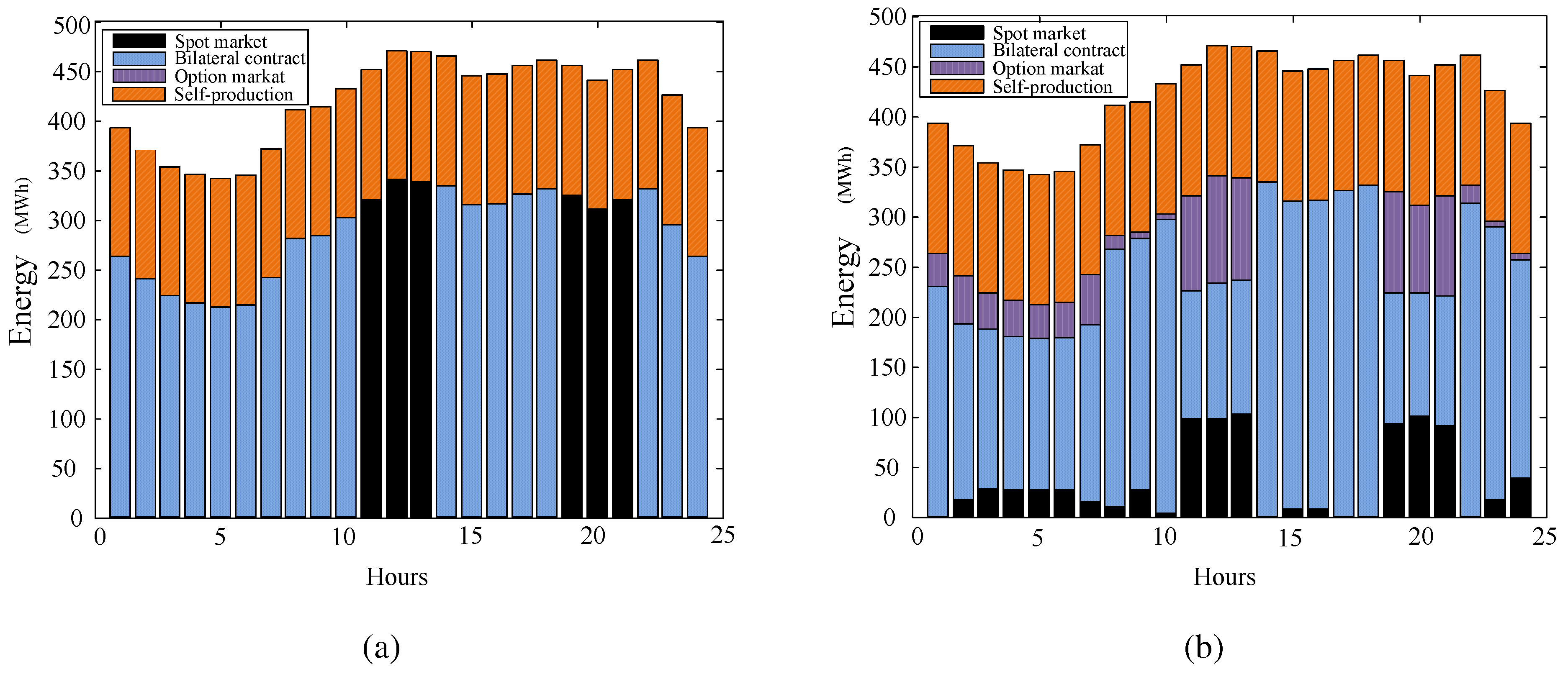
Figure 1. Energy procurement for two levels of risk ($\lambda =0,0.5$). (a) $\lambda =0$; (b) $\lambda =0.5$.

Figure 1. Energy procurement for two levels of risk ($\lambda =0,0.5$). (a) $\lambda =0$; (b) $\lambda =0.5$.

Figure 1 shows the energy procurement in a whole day with two different tradeoff coefficients. When $\lambda =0$, the large consumer decides the purchasing procurement with the aim of minimizing the purchasing cost. As can be seen in Figure 1a, the self-production facility operates in a whole day. During Hours 2–7 (valley period) and Hours 1, 8–10, 14–18 and 22–24 (shoulder period), bilateral contract prices are much smaller than the corresponding prices in the spot market and the options market; as a result, the remaining electricity is bought exclusively from bilateral contracts during these hours. On the other hand, during Hours 11–13 and 19–21 (peak period), mostenergy is bought from the spot market, because it has less expensive price. With the increasing of λ, the weight of risk in Equation (25) also increases. As shown in Figure 1b, when $\lambda =0.5$, the spot market participates in this trading during the valley and shoulder periods, and the options market can also obtain the purchase orders. The reason for this comes from the existence of the spot market and the options market being able to reduce the risk. A comparison between Figure 1a and Figure 1b shows the conclusion that the existence of polynary markets can help with risk reduction.

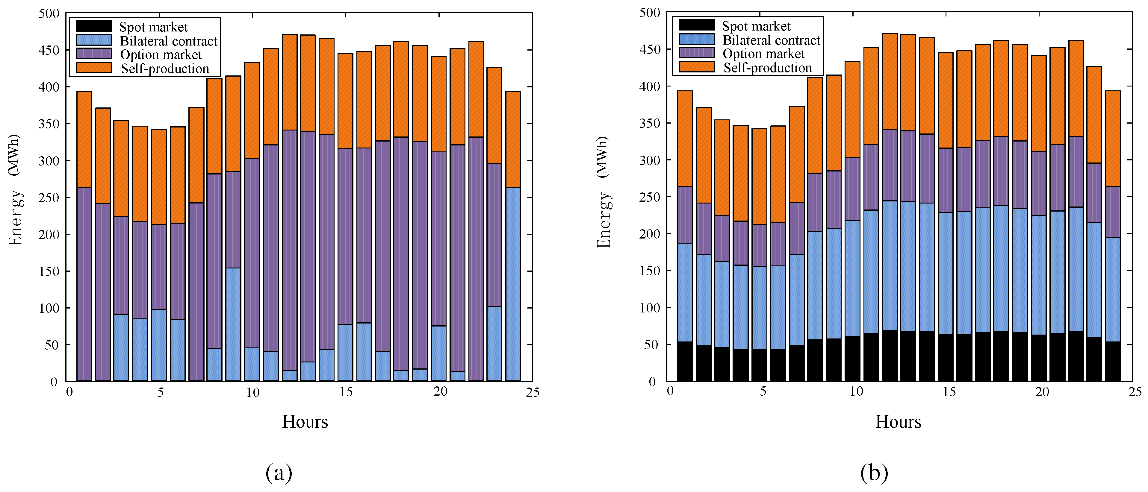
Figure 2. Comparison of energy procurement between considering the power quality and neglecting the power quality ($\lambda =1$); (a) neglecting power quality; (b) considering power quality.

Figure 2. Comparison of energy procurement between considering the power quality and neglecting the power quality ($\lambda =1$); (a) neglecting power quality; (b) considering power quality.

Figure 2 shows the comparison of energy procurement between the situations considering and neglecting power quality. When neglecting the influence of the fluctuation of power quality, electricity price is the only source of risk. When $\lambda =1$, electricity procurement is decided to minimize the risk; as Figure 2a shows, energy is purchased through a bilateral contract, the option market and self-production. When $\lambda =1$, risk is considered firstly; thus, no energy will be bought in the spot market because of its high uncertainty regarding the electricity price. However, taking power quality into consideration, risk becomes a complex of the uncertainty of the spot price and the fluctuation of power quality. The results in Figure 2b show that while the decision-making model considers the influence of the fluctuation of power quality, the purchasing percentage in each market changes greatly: the amount of energy sharply decreases in the options market, and on the other hand, a large amount of energy is purchased from the bilateral contract and the spot market. This phenomenon means that under the scenario of Figure 2b, the uncertainty of the electricity price is no longer the only risk factor: the fluctuation of the power quality also has a great influence on the decision of the power purchasing strategy.

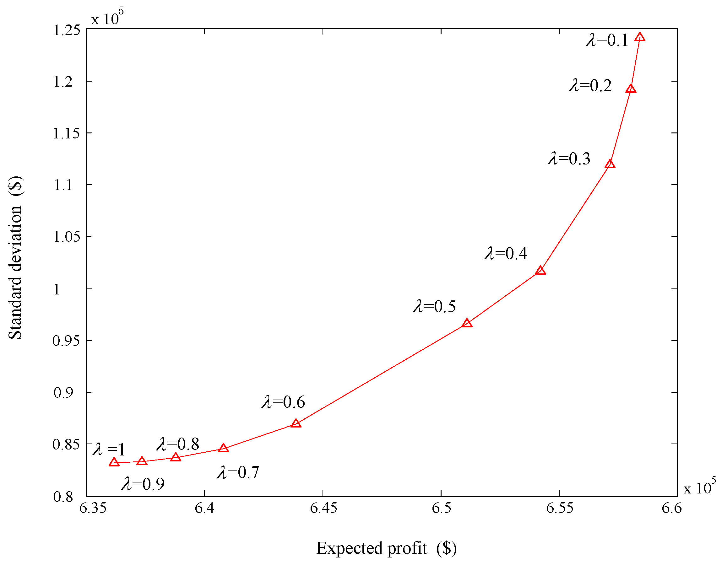
Figure 3. Expected profit against the profit standard deviation.

Figure 3. Expected profit against the profit standard deviation.

Another factor that influences the decision of the power purchasing strategy is the tradeoff between expected procurement profit and risk. Parameter λ, which is the tradeoff coefficient, lies in the range [0, 1]. With the increase of λ, the change of the expected profit and standard deviation is shown in Figure 3. From Figure 3, it can be observed that the expected profit decreases with the decreases of the standard deviation. Note that the value of λ depends on the preference of the consumer. When a large consumer wishes for a bigger expected procurement profit, then λ approaches zero. When a large consumer wishes for a smaller purchasing risk, then λ approaches one.

5. Conclusions

In the framework of an electricity market that includes the spot market, the options market and bilateral contract agreements and considering the fluctuation of power quality and the uncertainty of the electricity price, this paper analyzes the optimal procurement problem faced by a large consumer and provides a decision-making model based on expected utility and entropy. The proposed model provides a wide range of factors that influence the decision of energy procurement: all of the uncertain prices, the fluctuation of the power quality and the tradeoff coefficient are considered. The results from a virtual one-day case study indicate that the introduction of the fluctuation of the power quality can have a significant impact on the electricity quantity in each market: comparing the results that neglect the fluctuation of the power quality, more energy will be bought from the spot market and the bilateral contract when considering the fluctuation of the power quality. Additionally, the choice of λ can also affect the energy procurement; with the increasing of λ, more energy will be bought from the bilateral contract and the options market. Using the decision-making model, the consumer can evaluate the varieties of choices and choose the most appropriate one according to its preferences for expected utility and risk.