1. Introduction
After the introduction of the effective average action and its functional renormalization group equation for gravity [
1], detailed investigations of the nonperturbative renormalization group (RG) behavior of Quantum Einstein Gravity (QEG) have become possible [
1,
2,
3,
4,
5,
6,
7,
8,
9,
10,
11,
12,
13,
14,
15,
16,
17,
18,
19,
20,
21]. The exact RG equation underlying this approach defines a Wilsonian RG flow on a theory space which consists of all diffeomorphism invariant functionals of the metric
. The approach turned out to be an ideal setting for investigating the Asymptotic Safety scenario in gravity [
22,
23,
24,
25,
26,
27,
28,
29] and, in fact, substantial evidence was found for the nonperturbative renormalizability of Quantum Einstein Gravity. The theory emerging from this construction (“QEG”) is not a quantization of classical general relativity. Instead, its bare action corresponds to a nontrivial fixed point of the RG flow and is therefore a
prediction. The effective average action [
1,
30,
31,
32,
33,
34,
35,
36,
37,
38,
39] has crucial advantages as compared to other continuum implementations of the Wilson RG. In particular, it is closely related to the standard effective action and defines a family of effective field theories
labeled by the coarse graining scale
k. The latter property opens the door to a rather direct extraction of physical information from the RG flow, at least in single-scale cases: If the physical process or phenomenon under consideration involves only a single typical momentum scale
, it can be described by a tree-level evaluation of
, with
. The precision which can be achieved by this effective field theory description depends on the size of the fluctuations relative to the mean values. If they are large, or if more than one scale is involved, it might be necessary to go beyond the tree analysis. The RG flow of the effective average action, obtained by different truncations of theory space, has been the basis of various investigations of “RG improved” black hole and cosmological spacetimes [
40,
41,
42,
43,
44,
45,
46,
47,
48,
49,
50,
51,
52,
53,
54]. We shall discuss some aspects of this method below.
The purpose of this article is to review the main features of renormalization group improved cosmologies based upon a RG trajectory of QEG with realistic parameter values. As a direct consequence of the nontrivial RG fixed point which underlies Asymptotic Safety, the early Universe is found to undergo a phase of adiabatic inflationary expansion; it is a pure quantum effect and requires no inflaton field. Furthermore, we shall see that the quantum gravity effects provide a novel mechanism for the generation of entropy; in fact, they could easily account for the entire entropy of the present Universe in the massless sector.
Our presentation follow [
55] and [
56] to which the reader is referred for further details. A related investigation of “asymptotically safe inflation”, using different methods, has been performed by S. Weinberg [
57].
2. Entropy and the Renormalization Group
A special class of RG trajectories obtained from QEG in the Einstein-Hilbert approximation [
1], namely those of the “Type IIIa” [
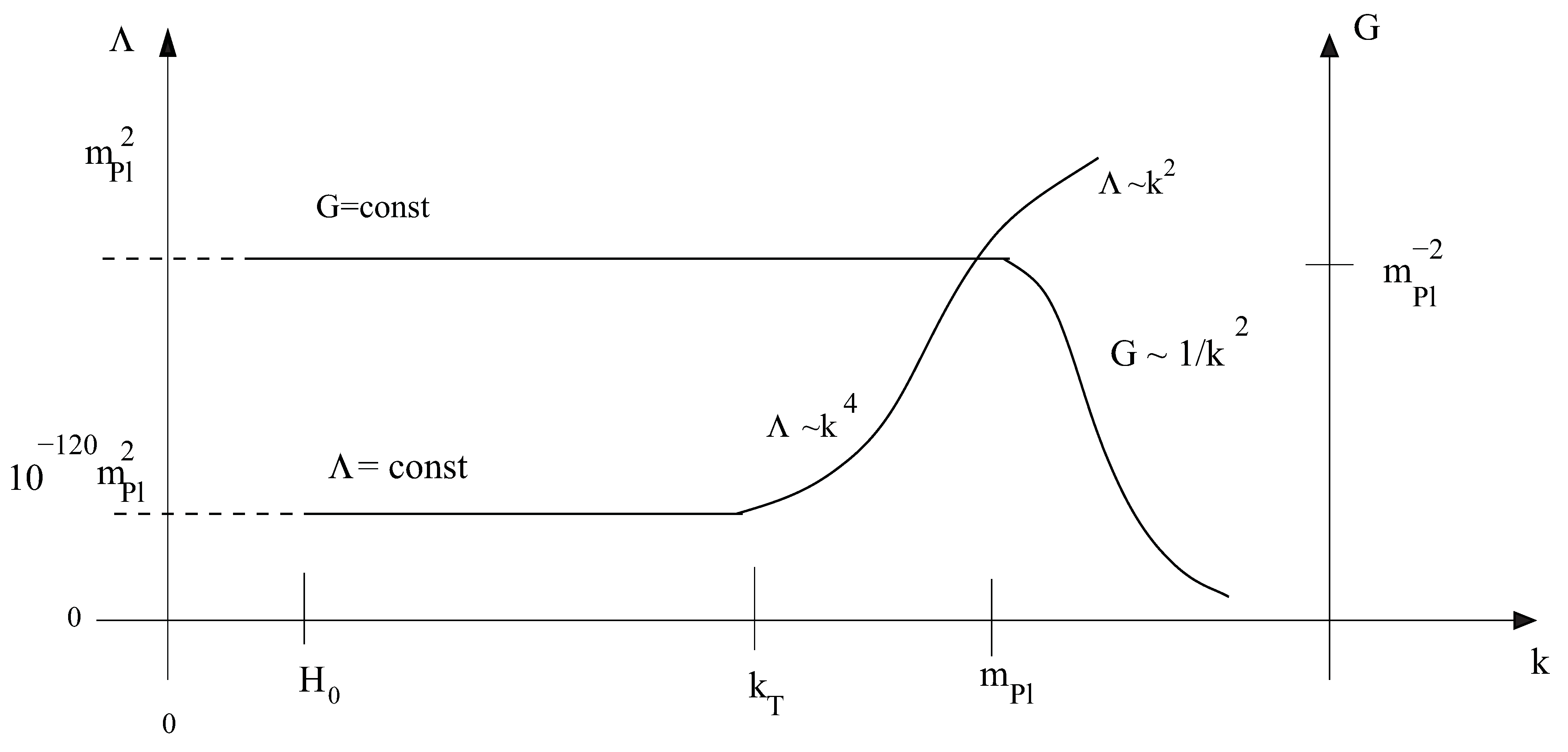
4], possess all the qualitative properties one would expect from the RG trajectory describing gravitational phenomena in the real Universe we live in. In particular they can have a long classical regime and a small, positive cosmological constant in the infrared (IR). Determining its parameters from observations, one finds [
55] that, according to this particular QEG trajectory, the running cosmological constant
changes by about 120 orders of magnitude between
k-values of the order of the Planck mass and macroscopic scales, while the running Newton constant
has no strong
k-dependence in this regime. For
, the non-Gaussian fixed point (NGFP) which is responsible for the Asymptotic Safety of QEG controls their scale dependence. In the deep ultraviolet
,
diverges and
approaches zero.
An immediate question is whether there is any experimental or observational evidence that would hint at this enormous scale dependence of the gravitational parameters, the cosmological constant in particular. Clearly the natural place to search for such phenomena is cosmology. Even though it is always difficult to give a precise physical interpretation to the RG scale k, it is fairly certain that any sensible identification of k in terms of cosmological quantities will lead to a k which decreases during the expansion of the Universe. As a consequence, will also decrease as the Universe expands. The purely qualitative assumption of a positive and decreasing cosmological constant already supplies an interesting hint as to which phenomena might reflect a possible Λ-running.
To make the argument as simple as possible, let us first consider a Universe without matter, but with a positive Λ. Assuming maximal symmetry, this is nothing but de Sitter space, of course. In static coordinates its metric is
with
In the weak field and slow motion limit
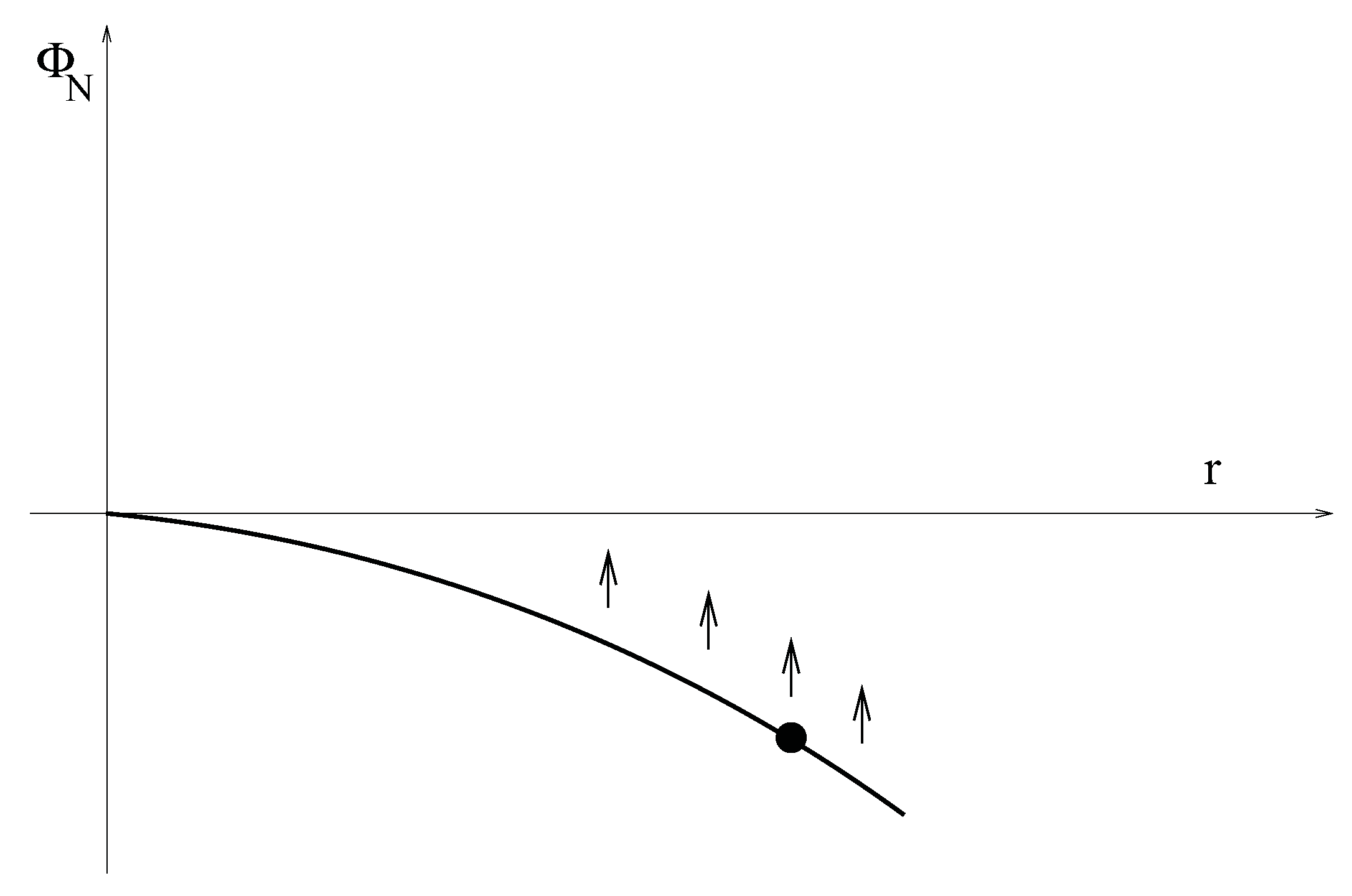
has the interpretation of a Newtonian potential, with a correspondingly simple physical interpretation. The left panel of
Figure 1 shows
as a function of
r; for
it is an upside-down parabola. Point particles in this spacetime, symbolized by the black dot in
Figure 1, “roll down the hill” and are rapidly driven away from the origin and from any other particle. Now assume that the magnitude of
is slowly (“adiabatically”) decreased. This will cause the potential
to move upward as a whole at decreasing slope. So the change in Λ increases the particle’s potential energy. This is the simplest way of understanding that a
positive decreasing cosmological constant has the effect of “pumping” energy into the matter degrees of freedom. More realistically one will describe the matter system in a hydrodynamics or quantum field theory language and one will include its backreaction onto the metric. But the basic conclusion, namely that a slow decrease of a positive Λ transfers energy into the matter system, will remain true.
Figure 1.
The quasi-Newtonian potential corresponding to de Sitter space is shown. The curve moves upward as the cosmological constant decreases.
Figure 1.
The quasi-Newtonian potential corresponding to de Sitter space is shown. The curve moves upward as the cosmological constant decreases.
We are thus led to suspect that, because of the decreasing cosmological constant, there is a continuous inflow of energy into the cosmological fluid contained in an expanding Universe. It will “heat up” the fluid or, more exactly, lead to a slower decrease of the temperature than in standard cosmology. Furthermore, by elementary thermodynamics, it will increase the entropy of the fluid. If during the time an amount of heat is transferred into a volume V at the temperature T, the entropy changes by an amount . To be as conservative (i.e., close to standard cosmology) as possible, we assume that this process is reversible. If not, is even larger.
In standard Friedmann-Robertson-Walker (FRW) cosmology the expansion is adiabatic, the entropy (within a comoving volume) is constant. Therefore it has always been somewhat puzzling where the huge amount of entropy contained in the present Universe comes from. Presumably it is dominated by the CMBR photons which contribute an amount of about to the entropy within the present Hubble sphere. (We use units such that . ) In fact, if it is really true that no entropy is produced during the expansion then the Universe would have had an entropy of at least immediately after the initial singularity which for various reasons seems quite unnatural. In scenarios which invoke a “tunneling from nothing”, for instance, spacetime was “born” in a pure quantum state, so the very early Universe is expected to have essentially no entropy. Usually it is argued that the entropy present today is the result of some sort of “coarse graining” which, however, typically is not considered an active part of the cosmological dynamics in the sense that it would have an impact on the time evolution of the metric, say.
Following [
55] we shall argue that in principle the entire entropy of the massless fields in the present universe can be understood as arising from the mechanism described above. If energy can be exchanged freely between the cosmological constant and the matter degrees of freedom, the entropy observed today is obtained precisely if the initial entropy at the “big bang” vanishes. The assumption that the matter system must allow for an unhindered energy exchange with Λ is essential, see [
44,
55].
We shall model the matter in the early Universe by a gas with
bosonic and
fermionic massless degrees of freedom, all at the same temperature.
In equilibrium its energy density, pressure, and entropy density are given by the usual relations (
)
so that in terms of
In an out-of-equilibrium process of entropy generation the question arises how the various thermodynamical quantities are related then. To be as conservative as possible, we make the assumption that the irreversible inflow of energy destroys thermal equilibrium as little as possible in the sense that the equilibrium relation (1) continue to be (approximately) valid.
This kind of thermodynamics in an FRW-type cosmology with a decaying cosmological constant has been analyzed in detail by Lima [
58], see also [
59]. It was shown that if the process of matter creation
gives rise to constant specific entropy per particle, the relations of equilibrium thermodynamics are preserved. This means that no finite thermalization time is required since the particles originating from the decaying vacuum are created in equilibrium with the already existing ones. Under these conditions it is also possible to derive a generalized black body spectrum which is conserved under time evolution. Such minimally non-adiabatic processes were termed “adiabatic” (with the quotation marks) in [
58,
59].
3. Asymptotically Safe Inflation
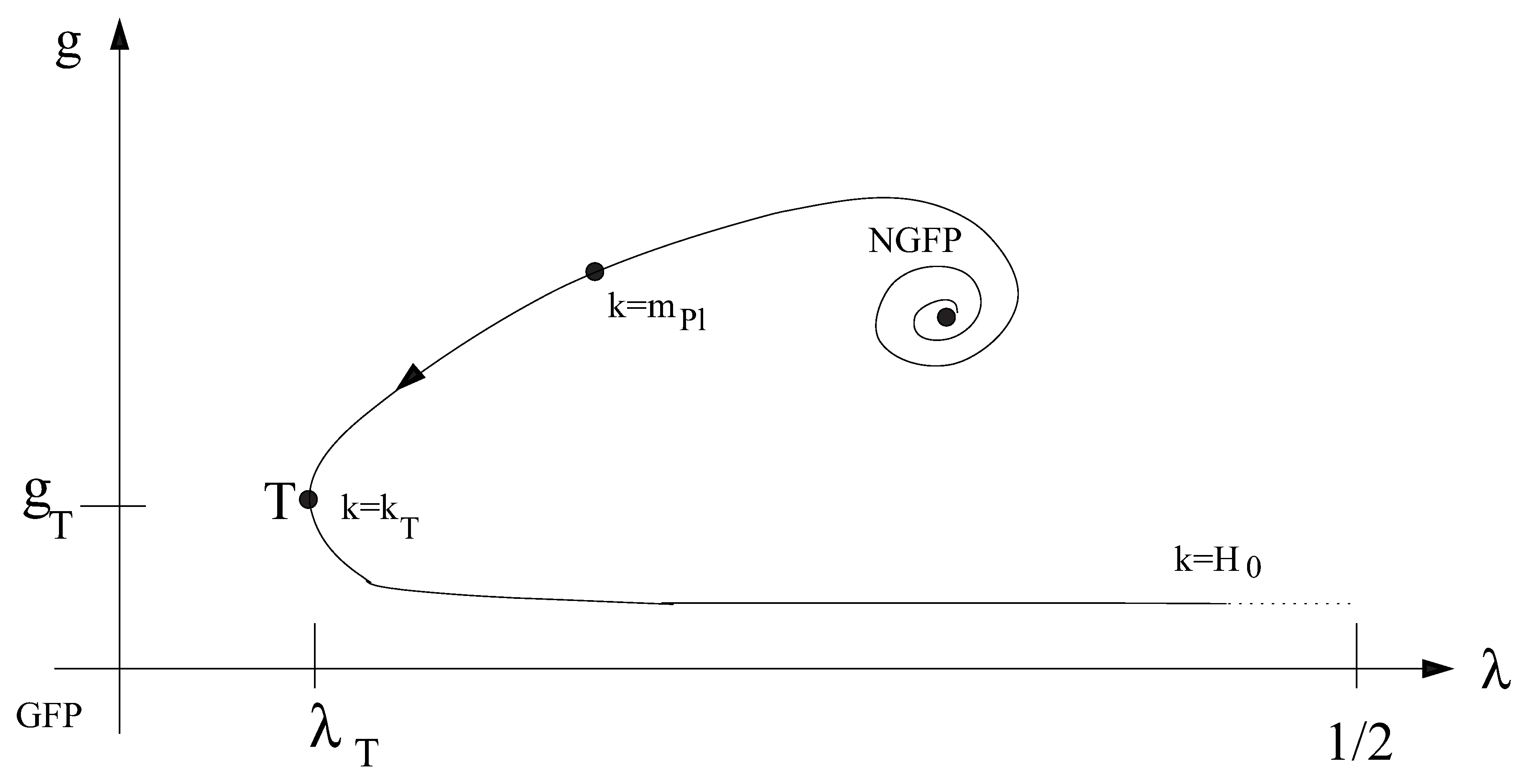
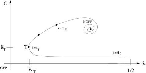
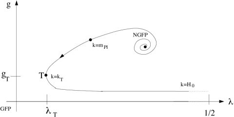
There is another, more direct potential consequence of a decreasing positive cosmological constant which we shall also explore here, namely a period of automatic inflation during the very first stages of the cosmological evolution. In the very early Universe the RG running of the gravitational parameters is governed by the non-Gaussian RG fixed point which is at the heart of the Asymptotic Safety scenario as shown in
Figure 2.
Figure 2.
The “realistic” RG trajectory discussed in the text, emanating from the NGFP, is shown. In particular is the momentum scale k at which the flow spends most of its “RG-time” near the GFP, so that the the dimensionful coupling constant approaches its classical values. The Planck scale indicates the crossover scale from the NGFP to the Gaussian fixed point.
The inflationary phase we are going to describe is a rather direct consequence of the huge cosmological constant which the NGFP enforces during the epoch governed by the asymptotic scaling regime of the renormalization group.
It is not surprising, of course, that a positive Λ can cause an accelerated expansion, but in the classical context the problem with a Λ-driven inflation is that it would never terminate once it has started. In popular models of scalar driven inflation this problem is circumvented by designing the inflaton potential in such a way that it gives rise to a vanishing vacuum energy after a period of “slow roll”.
As we shall see generic RG cosmologies based upon the QEG trajectories have an era of Λ-driven inflation immediately after the big bang which ends automatically as a consequence of the RG running of . Once the scale k drops significantly below , the accelerated expansion ends because the vacuum energy density is already too small to compete with the matter density. Clearly this is a very attractive scenario: to neither trigger inflation nor stop it, one needs any ad hoc ingredients such as an inflaton field or a special potential. It suffices to include the leading quantum effects in the gravity and matter system. Furthermore, asymptotic safety offers a natural mechanism for the quantum mechanical generation of primordial density perturbations, the seeds of cosmological structure formations.
In the following we review a concrete investigation along these lines. For further details we refer to [
44,
55].
4. The Improved Einstein Equations
The computational setting of our investigation [
55] are the RG improved Einstein equations: By means of a suitable cutoff identification
we turn the scale dependence of
and
into a time dependence, and then substitute the resulting
and
into the Einstein equations
. We specialize
to describe a spatially flat
Robertson-Walker metric with scale factor
, and we take
to be the energy momentum tensor of an ideal fluid with equation of state
where
is constant. Then the improved Einstein equation boils down to the modified Friedmann equation and a continuity equation:
The modified continuity equation (
2b) is the integrability condition for the improved Einstein equation implied by Bianchi’s identity,
. It describes the energy exchange between the matter and gravitational degrees of freedom (geometry). For later use let us note that upon defining the critical density
and the relative densities
and
the modified Friedmann equation (
2a) can be written as
.
We shall obtain
and
by solving the flow equation in the Einstein-Hilbert truncation with a sharp cutoff [
1,
4]. It is formulated in terms of the dimensionless Newton and cosmological constant, respectively:
,
. We then construct quantum corrected cosmologies by (numerically) solving the RG improved evolution equations. We shall employ the cutoff identification
where
ξ is a fixed positive constant of order unity. This is a natural choice since in a Robertson-Walker geometry the Hubble parameter measures the curvature of spacetime; its inverse
defines the size of the “Einstein elevator”. Thus we have
One can prove that all solutions of the coupled system of differential equations (
2a),
2b) can be obtained by means of the following algorithm:
Let be a prescribed RG trajectory and a solution ofLet be defined in terms of this solution byThen the pair is a solution of the system (
2a), (
2b)
for the time dependence of G and Λ given by (
4)
and the equation of state , provided . 5. RG Trajectory with Realistic Parameter Values
Before we start solving the modified field equations let us briefly review how the type IIIa trajectories of the Einstein-Hilbert truncation can be matched against the observational data [
40]. This analysis is fairly robust and clear-cut; it does not involve the NGFP. All that is needed is the approximate RG flow about the Gaussian fixed point (GFP) which is located at
. In its vicinity one has [
1]
and
. Or, in terms of the dimensionless couplings,
,
. In the linear regime of the GFP, Λ displays a running
and
G is approximately constant. Here
ν is a positive constant of order unity [
1,
4]. These equations are valid if
and
. They describe a 2-parameter family of RG trajectories labeled by the pair
. It will prove convenient to use an alternative labeling
with
and
. The old labels are expressed in terms of the new ones as
and
. It is furthermore convenient to introduce the abbreviation
. When parameterized by the pair
the trajectories assume the form
or, in dimensionless form,
As for the interpretation of the new variables, it is clear that
and
, while
is the scale at which
(but not
) vanishes according to the linearized running:
. Thus we see that
are the coordinates of the turning point T of the type IIIa trajectory considered, and
is the scale at which it is passed. It is convenient to refer the “RG time”
τ to this scale:
. Hence
(
) corresponds to the “UV regime” (“IR regime”) where
(
.
Let us now hypothesize that, within a certain range of
k-values, the RG trajectory realized in Nature can be approximated by (
8). In order to determine its parameters
or
we must perform a measurement of
G and Λ. If we interpret the observed values
,
, and
as the running
and
evaluated at a scale
, then we get from (
7) that
and
. Using the definitions of
and
along with
this leads to the order-of-magnitude estimates
and
. Because of the tiny values of
and
the turning point lies in the linear regime of the GFP.
Up to this point we discussed only that segment of the “trajectory realized in Nature” which lies inside the linear regime of the GFP. The complete RG trajectory is obtained by continuing this segment with the flow equation both into the IR and into the UV, where it ultimately spirals into the NGFP. While the UV-continuation is possible within the Einstein-Hilbert truncation, this approximation breaks down in the IR when
approaches
. Interestingly enough, this happens near
, the present Hubble scale. The right panel of
Figure 1 shows a schematic sketch of the complete trajectory on the
g-
λ–plane and
Figure 2 displays the resulting
k-dependence of
G and Λ.
6. Primordial Entropy Generation
Let us return to the modified continuity equation (
2b). After multiplication by
it reads
where we defined
Without assuming any particular equation of state equation (
9) can be rewritten as
The interpretation of this equation is as follows. Let us consider a unit
coordinate,
i.e., comoving volume in the Robertson-Walker spacetime. Its corresponding
proper volume is
and its energy contents is
. The rate of change of these quantities is subject to (
11):
In classical cosmology where
this equation together with the standard thermodynamic relation
is used to conclude that the expansion of the Universe is adiabatic,
i.e., the entropy inside a comoving volume does not change as the Universe expands,
.
In the following we shall write for the entropy carried by the matter inside a unit comoving volume and s for the corresponding proper entropy density.
When Λ and
G are time dependent,
is nonzero and we interpret (
12) as describing the process of energy (or “heat”) exchange between the scalar fields Λ and
G and the ordinary matter. This interaction causes
S to change:
The actual rate of change of the comoving entropy is
where
If
T is known as a function of
t we can integrate (
13) to obtain
. In the RG improved cosmologies the entropy production rate per comoving volume
is nonzero because the gravitational “constants” Λ and
G have acquired a time dependence.
For a given solution to the coupled system of RG and cosmological equations it is sometimes more convenient to calculate
from the LHS of the modified continuity equation rather than its RHS (
16):
If
S has to increase with time, by (
16), we need that
. During most epochs of the RG improved cosmologies we have
and
. The decreasing Λ and the increasing
G have antagonistic effects therefore. We shall see that in the physically realistic cases Λ predominates so that there is indeed a transfer of energy from the vacuum to the matter sector rather than vice versa.
Clearly we can convert the heat exchanged, , to an entropy change only if the dependence of the temperature T on the other thermodynamical quantities, in particular ρ and p is known. For this reason we shall now make the following assumption about the matter system and its (non-equilibrium!) dynamics:
The matter system is assumed to consist of species of effectively massless degrees of freedom which all have the same temperature T. The equation of state is ,i.e.
, , and ρ depends on T asNo assumption is made about the relation . The first assumption, radiation dominance and equal temperature, is plausible since we shall find that there is no significant entropy production any more once has dropped substantially below , after the crossover from the NGFP to the GFP.
The second assumption, Equation (
18), amounts to the hypothesis formulated in the introduction. While entropy generation is a non-adiabatic process we assume, following Lima [
58], that the non-adiabaticity is as small as possible. More precisely, the approximation is that the
equilibrium relations among
ρ,
p, and
T are still valid in the non-equilibrium situation of a cosmology with entropy production. In this sense, (
18) is the extrapolation of the standard relation (
1a) to a “slightly non-adiabatic” process.
Note that while we used (1c) in relating
to the entropy production and also postulated Equation (
1a), we do not assume the validity of the formula for the entropy density, Equation (
1b), a priori. We shall see that the latter is an automatic consequence of the cosmological equations.
To make the picture as clear as possible we shall neglect in the following all ordinary dissipative processes in the cosmological fluid.
Using
and (
18) in (
17) the entropy production rate can be evaluated as follows:
Remarkably,
turns out to be a total time derivative:
Therefore we can immediately integrate Equation (
13) and obtain
or, in terms of the proper entropy density,
Here
is a constant of integration. In terms of
T, using Equation (
18) again,
The final result (
23) is very remarkable for at least two reasons. First, for
, Equation (
23) has exactly the form (1b) which is valid for radiation in equilibrium. Note that we did not postulate this relationship, only the
–law was assumed. The equilibrium formula
was
derived from the cosmological equations,
i.e., the modified conservation law. This result makes the hypothesis “non-adiabatic, but as little as possible” self-consistent.
Second, if
, which is actually the case for the most interesting class of cosmologies, then we shall find
by Equation (
21). As we mentioned in the introduction, the most plausible initial value of
S is
which means a vanishing constant of integration
here. But then, with
, (
21) tells us that the
entire entropy carried by the massless degrees of freedom is due to the RG running. So it indeed seems to be true that the entropy of the CMBR photons we observe today is due to a coarse graining but, unexpectedly, not a coarse graining of the matter degrees of freedom but rather of the gravitational ones which determine the background spacetime the photons propagate on.
We close this section with various comments. As for the interpretation of the function , let us remark that it also measures the deviations from the classical laws and , respectively, since we have .
In the improved cosmology the “consistency condition” implies the quantity
is conserved in time [
44]. If energy transfer is permitted and the entropy of the ordinary matter grows,
increases as well. This is obvious from
or, in integrated form,
.
In a spatially flat Robertson-Walker spacetime the overall scale of
has no physical significance. If
is time independent, we can fix this gauge ambiguity by picking a specific value of
and expressing
correspondingly. For instance, parametrized in this way, the scale factor of the classical FRW cosmology with
,
reads [
44]
If, during the expansion,
increases slowly, Equation (
25) tells us that the expansion is actually
faster than estimated classically. Of course, what we actually have to do in order to find the corrected
is to solve the improved field equations and not insert
into the classical solution, in particular when the change of
is not “slow”. Nevertheless, this simple argument makes it clear that entropy production implies an increase of
which in turns implies an extra increase of the scale factor. This latter increase, or “inflation”, is a pure quantum effect. The explicit solutions to which we turn next will confirm this picture.
7. Solving the RG Improved Einstein Equations
In [
55] we solved the improved Einstein Equation (
2a),
2b) for the trajectory with realistic parameter values which was discussed in
Section 5. The solutions were determined by applying the algorithm described at the end of
Section 4. Having fixed the RG trajectory, there exists a 1-parameter family of solutions
. This parameter is conveniently chosen to be the relative vacuum energy density in the fixed point regime,
.
The very early part of the cosmology can be described analytically. For
the trajectory approaches the NGFP,
, so that
and
. In this case the differential equation can be solved analytically, with the result
and
Here
A,
,
, and
are positive constants. They depend on
which assumes values in the interval
. If
the deceleration parameter
is negative and the Universe is in a phase of
power law inflation. Furthermore, it has
no particle horizon if
, but does have a horizon of radius
if
. In the case of
this means that there is a horizon for
, but none if
.
If
, the above discussion of entropy generation applies. The corresponding production rate reads
For the entropy per unit comoving volume we find, if
,
and the corresponding proper entropy density is
For the discussion of the entropy we must distinguish 3 qualitatively different cases.
(a) The case , i.e., : Here
so that the entropy and energy content of the matter system increases with time. By Equation (
16),
implies
. Since
but
in the NGFP regime, the energy exchange is predominantly due to the decrease of Λ while the increase of
G is subdominant in this respect.
The comoving entropy has a finite limit for , , and grows monotonically for . If , which would be the most natural value in view of the discussion in the introduction, all of the entropy carried by the matter fields is due to the energy injection from Λ.
(b) The case , i.e., : Here so that the energy and entropy of matter decreases. Since amounts to , the dominant physical effect is the increase of G with time, the counteracting decrease of Λ is less important. The comoving entropy starts out from an infinitely positive value at the initial singularity, . This case is unphysical probably.
(c) The case , : Here , . The effect of a decreasing Λ and increasing G cancel exactly.
At lower scales the RG trajectory leaves the NGFP and very rapidly “crosses over” to the GFP at
, as it is shown in
Figure 2. This is most clearly seen in the behavior of the anomalous dimension
which quickly changes from its NGFP value
to the classical
. This transition happens near
or, since
, near a cosmological “transition” time
defined by the condition
. (Recall that
). The complete solution to the improved equations can be found with numerical methods only. It proves convenient to use logarithmic variables normalized with respect to their respective values at the turning point. Besides the “RG time"
, we use
,
, and
.
Summarizing the numerical results one can say that for any value of the UV cosmologies consist of two scaling regimes and a relatively sharp crossover region near corresponding to which connects them. At higher k-scales the fixed point approximation is valid, at lower scales one has a classical FRW cosmology in which Λ can be neglected.
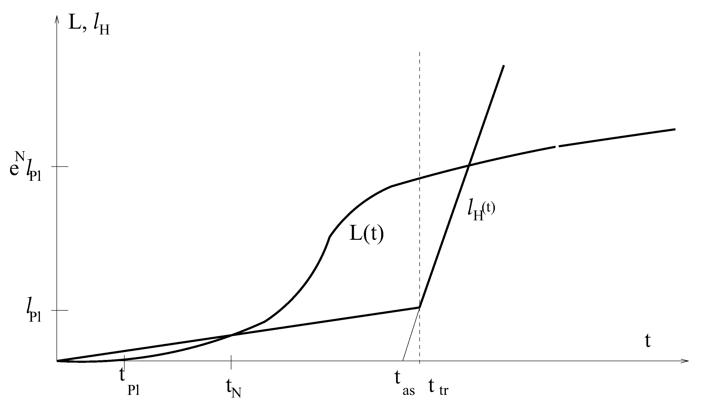
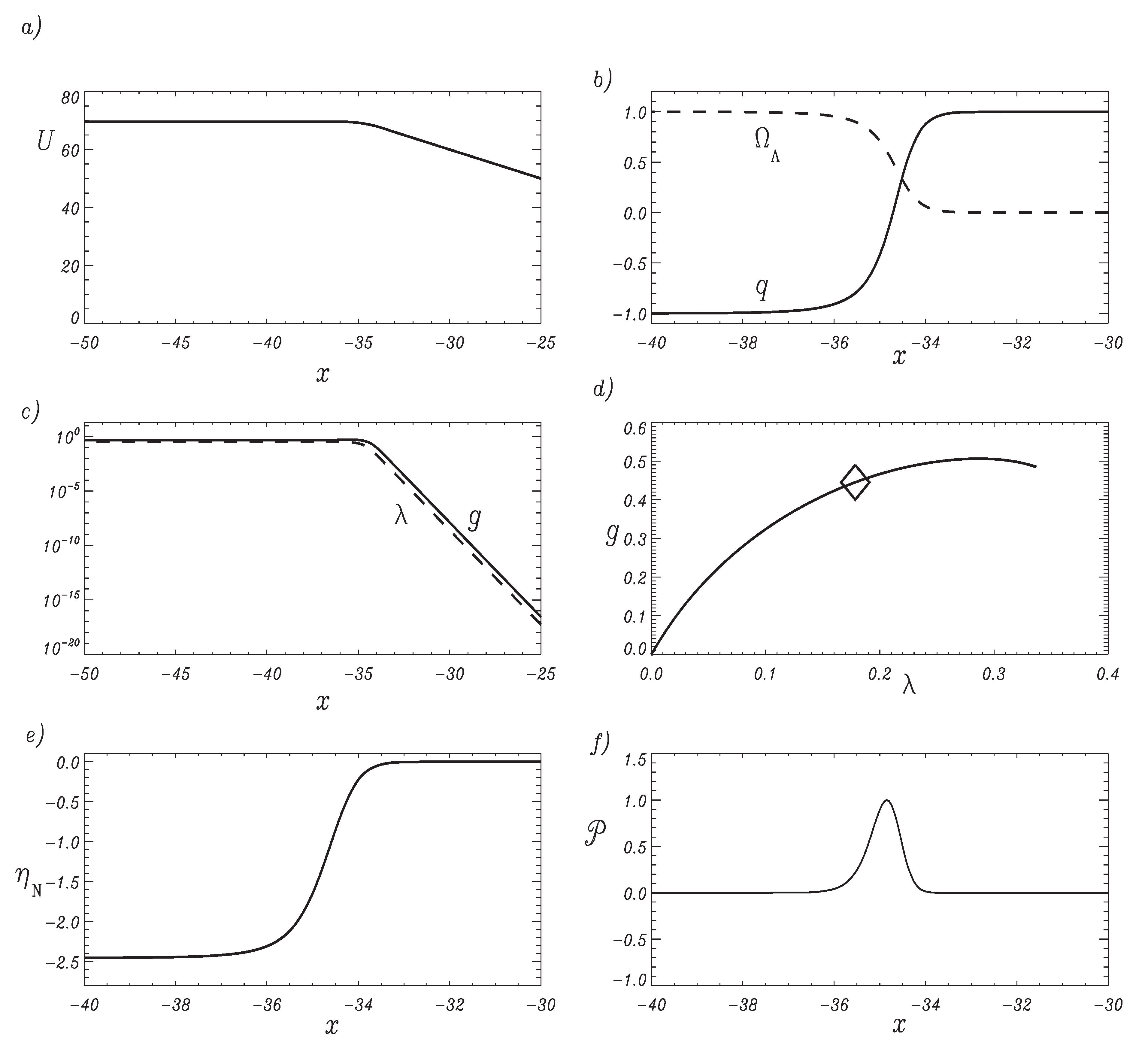
As an example,
Figure 3 shows the crossover cosmology with
and
. The entropy production rate
is maximum at
and quickly goes to zero for
; it is non-zero for all
. By varying the
-value one can check that the early cosmology is indeed described by the NGFP solution (5.1). For the logarithmic
H vs.
a- plot, for instance, it predicts
for
. The left part of the plot in
Figure 3a and its counterparts with different values of
indeed comply with this relation. If
we have
and
describes a phase of accelerated power law inflation.
Figure 3.
The dimensionful quantities and for the RG trajectory with realistic parameter values.
Figure 3.
The dimensionful quantities and for the RG trajectory with realistic parameter values.
When , the slope of decreases and finally vanishes at . This limiting case corresponds to a constant Hubble parameter, i.e., to de Sitter space. For values of smaller than, but close to 1 this de Sitter limit is approximated by an expansion with a very large exponent α.
The phase of power law inflation automatically comes to a halt once the RG running has reduced Λ to a value where the resulting vacuum energy density no longer can overwhelm the matter energy density.
