Abstract
Using panel data of 30 provinces and regions in Mainland China (excluding Tibet) from 2006 to 2016, the Spatial Durbin Model was employed for the empirical research, and the spatial impact of fiscal decentralization and environmental decentralization on regional carbon emissions were analyzed from the perspective of promotion pressure of officials. The empirical study concludes: ① Fiscal decentralization, both within the region and in its neighborhood, will contribute to carbon emissions in the region; ② Environmental decentralization will help reduce carbon emissions, while environmental decentralization in neighboring regions will increase carbon emissions in the region; ③ The promotion pressure of officials plays a positive role in moderating the impact of fiscal decentralization on carbon emissions, and at the same time weakens the suppression of carbon emissions by environmental decentralization; ④ From a regional point of view, there is a positive relationship between fiscal decentralization and carbon emissions in various regions; but environmental decentralization has obvious spatial heterogeneity. The research suggests that reducing the degree of local fiscal decentralization, investment in major infrastructure projects involving high carbon emissions should be relatively centralized; appropriately increase the environmental management authority of local environmental protection agencies, fully use the advantages of local environmental protection departments to protect the environment according to local conditions; gradually improve the assessment system for local officials, moderately reduce the proportion of fiscal revenue and GDP assessment in areas with fragile ecological environment, and increase incentives for ecological performance assessment, put the development of low-carbon economy into practice.
1. Introduction
As the largest industrial producing country in the world, Chinese industrial production will lead to high carbon emissions, and coal consumption is the main source of carbon emissions, while the energy resources of China are precisely characterized as “coal-rich, oil-poor and gas-lean”. According to public data from the “Global Carbon Atlas”, China accounted for 27.5% of global carbon emissions in 2018 [1], making it the most affected country in terms of global air pollution. The Chinese government attaches great importance to this issue. In order to accelerate green and low-carbon development, the State Council issued the “13th Five-Year Plan for Controlling Greenhouse Gas Emissions” in 2016 to push China’s carbon emissions reach to the peak point around 2030 as fast as possible.
The environmental problems (especially carbon emissions) in China are not only caused by technical and financial reasons, but also the result of distorted incentives and insufficient constraints under the decentralization system of the government [2]. The majority of the literature on carbon emissions has been examined from the perspectives of GDP per capita, intensity of environmental regulations, energy mix, population size, level of urbanization, industrial structure, corruption and foreign direct investment etc. [3,4,5,6,7,8,9]. However, the government’s decentralization system is often ignored due to its indirect and difficult to evaluate the impact on energy conservation and emission reduction [10]. As a typical environmental public good, carbon emission has obvious negative externalities, so it is very necessary for the government to intervene in. Yet the effectiveness of the current government’s decentralized management system has been debated in academics.
China is a country with a decentralization system which includes both fiscal decentralization and environmental decentralization. Fiscal decentralization studies the attribution of central and local economic rights. The key point is to analyze the supply efficiency of public goods and its relationship with economic growth. It mainly reflects the incentive mechanism combining “political centralization and economic decentralization” [11], while environmental decentralization focuses on the division of environmental management authority. It mainly includes the division of authority between central and local governments for setting environmental standards, administrative punishment, administrative permit approval, environmental quality monitoring and evaluation, and environmental law enforcement inspection [12]. They are interrelated but have essential differences. At the provincial level, local environmental protection departments are under dual jurisdiction and are restricted by local governments in terms of personnel and finance. The relationship between fiscal decentralization and environmental decentralization is shown in Figure 1. Most studies simply use fiscal decentralization as a proxy indicator of environmental decentralization, which will lead to errors in the measurement of variables and the estimation results.
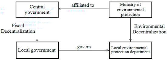
Figure 1.
The relationship between fiscal decentralization and environmental decentralization.
Moreover, unlike the official election system in Western countries, local officials in China are judged and appointed by higher authorities based on a range of indicators, particularly economic ones. As a result, local officials are likely to lower environmental standards for the sake of their own promotion in order to ensure economic growth. In other words, the huge promotion pressure faced by local officials will affect the efficiency and effect of the implementation of environmental laws and policies, and then affect the mechanism of decentralization on carbon emissions [13,14]. Although the Chinese government has issued a series of important laws and regulations on environmental protection, environmental problems remain a common problem. Therefore, the implementation of local officials’ responsibility for environmental policies deserves intensive attention.
This paper focuses on the study of the effect of Chinese decentralization on carbon emissions, which intends to address the following questions: Is the influence on carbon emission from fiscal decentralization the same as the environmental decentralization? Is there a spatial effect of decentralization on carbon emissions? Is there a regional heterogeneity? What is the moderating effect of officials’ promotion pressure on the impact of decentralization on carbon emissions? To solve these issues is called upon to take an overall consideration from the perspective of the coordination between the government decentralization system and environmental protection. At present, the contradiction between economic growth and the preservation of environment is prominent, so the study of carbon emission in the context of decentralization system reform is of great significance to the reform of environmental governance.
2. Literature Review and Theoretical Hypothesis
2.1. Fiscal Decentralization and Carbon Emissions
Fiscal decentralization refers to the central government giving local governments a certain range of taxation powers and expenditure responsibilities and allowing them to determine the scale and structure of their budget expenditures on their own, so that local governments can participate more actively in social management. China’s fiscal decentralization system has been formed since the implementation of the tax sharing reform in 1994. It has greatly stimulated the competition of local governments in economic construction and created the myth of China’s rapid economic growth in the past 30 years [15]. There are various conclusions about the impact of fiscal decentralization on carbon reduction and environmental quality, which can be roughly divided into: (1) Inhibition theory. Most scholars, such as Sigman [16], Woods [17], Kang [18] and Zhang [19], support the “race to bottom competition” theory that fiscal decentralization leads to a decline in environmental quality. They argue that when there is competition between jurisdictions, local governments will actively lower environmental standards in order to attract capital inflows and increase tax revenues, leading to a deterioration in environmental quality, which can lead to environmental problems such as the tragedy of the commons, the pollution “border effect”, incidents of toxic land and the “neighbourhood avoidance effect “. (2) Promotion theory. Another group of scholars, such as Magnani [20], Gray [21] and Konisky [4] have argued that local governments can tailor more appropriate and individualized environmental public services to the spatial heterogeneity of different jurisdictions, thus creating a “race to top” competition in environmental quality. (3) Irrelevance theory. Few scholars [22,23] have argued that there is no necessary link between fiscal decentralization and environmental quality. Although the above views have been confirmed by the empirical data of some countries or regions, the understanding of the impact of fiscal decentralization on China’s carbon emissions is still insufficient.
Under the fiscal decentralization system, local governments rely heavily on the “auction” of land to obtain large amounts of land concessions. On one hand, this leads to the rapid development of the real estate sector, and on the other hand, local governments are incentivized by economic performance assessments to use the land concessions to develop public infrastructure. However, both the real estate and infrastructure development will lead to a sharp rise in carbon emissions. Carbon emission is a pollutant with strong spillover and no obvious harm in the short term, and its governance cost and benefit are not equal, decentralization will reduce the control effect of local government on carbon emission [19]. In order to achieve economic growth, the competing local governments tend to imitate each other, resulting in a “free-riding” phenomenon that leads to a downward competition in carbon reduction efficiency. Based on this, this paper proposes the first hypothesis:
Hypothesis 1 (H1).
Fiscal decentralization is positively related to carbon emissions in the region, i.e., the higher the degree of fiscal decentralization, the more carbon emissions will be emitted in the region; an increase in fiscal decentralization in neighbouring regions will increase carbon emissions in the region.
2.2. Environmental Decentralization and Carbon Emissions
The core of environmental management system reform is to reasonably allocate environmental protection power among different levels of government, that is, to determine the appropriate degree of environmental decentralization [24]. In 1956, Tiebout [25] proposed the famous “decentralization theorem”, arguing that decentralization can increase the efficiency of public goods, and residents can force local governments to provide public goods that can better meet the heterogeneous preferences of residents in different districts through “voting with their feet”. This argument laid the theoretical foundation for the decentralization system. Since the 1970s, an environmental federalism theory has gradually formed, which is rooted in the theory of fiscal decentralization [26], It aims to seek the optimal allocation of environmental management power among government levels [27], and is considered as the “key prescription” to solve environmental problems [16,28]. After that, the research on the relationship between environmental decentralization and environmental governance has gradually increased and formed two opposite views of “race to top” and “race to bottom” [16,28,29,30,31,32]. However, the research on the impact of environmental decentralization on carbon emission is still insufficient.
Since the 21st century, China’s economy has shifted from “a stage of high-speed growth to a stage of high-quality development”. High quality requires a sustainable economic development and an unprecedented level of ecological protection. It is necessary to explore the institutional factors affecting carbon emissions from the perspective of environmental management system. Local governments generally have a better understanding of local residents’ preferences for public goods such as ecological environment, and a decentralized environmental management system is more conducive for local environmental protection departments to comprehensively consider various factors according to the actual situation and select the most appropriate emission reduction scheme, so as to manage the local ecological environment in a “localized manner” [33].With the increase of the degree of environmental decentralization, the arrangement of local environmental protection institutions and personnel increases, which is more conducive to the local government to carry out environmental governance, testing, supervision and inspection, and can address the problem of carbon emissions more effectively. Furthermore, as the weight of ecological performance assessment increases, environmental protection departments in neighbouring regions will adopt a competitive strategy of imitating each other to improve the environment, leading to a “race to top” in environmental quality [29]. For this reason, this paper proposes the second hypothesis:
Hypothesis 2 (H2).
Environmental decentralization is conducive to curbing carbon emissions in the region; and an increase in the degree of environmental decentralization in neighbouring regions will also contribute to carbon reduction in the region.
2.3. Moderating Effect of Officials’ Promotion Pressure on the Effectiveness of Decentralization System
The “key minority” of leading cadres is essential to the success of ecological civilization. China’s fiscal decentralization is accompanied by political centralization, which profoundly affects the attitude of economic decentralization to the ecological environment. Political centralization determines whether local officials are promoted politically [34]. The promotion pressure of officials will affect the efforts of local governments to implement environmental policies through the discretion of the decentralization system, thus indirectly affecting the level of carbon emissions [35]. In the past, the central government has been using a GDP-driven assessment mechanism to evaluate local governments for a long time, and this promotion incentive has given local officials a very strong incentive to promote rapid local GDP development [36]. In the decentralized system, local officials are constrained by limited budgets to invest in environmental projects that require large investments, have long lead times and are difficult to return in the short term, and carbon emissions have significant negative externalities across regions, making the benefits and costs of carbon emissions reduction unequal. As the result, most local officials have opted for a “free-rider” approach to carbon emissions, and have even taken on the role of “entrepreneurs” in implementing local decisions [37].
Despite the important role that environmental decentralization plays in curbing carbon emissions as an institutional influence on environmental quality [38], the pressure for promotion faced by local officials can affect the effect of environmental decentralization on carbon emissions via influencing the enforcement of environmental protection systems. Due to the pressure for promotion, local officials tend to use their discretionary power in economic decision-making to focus on economic development, while not monitoring and managing energy conservation and emission reduction enough, and investment in ecological and environmental management still gives way to competition for GDP growth. Recently, the central government has begun to pay close attention to environmental protection and has gradually incorporated energy conservation and emission reduction into the performance appraisal system for officials, but this ecological performance appraisal still gives local governments greater discretionary power, and the ecological performance appraisal suffers from a lack of incentives. In addition, local officials are generally only responsible for environmental problems in their own jurisdictions during their term of office, and the average term of office of local officials is generally not very long, so officials are driven by “promotion” during their term of office, and the phenomenon of pollution for the sake of promotion exists. Therefore, this paper proposes the following hypotheses:
Hypothesis 3 (H3).
Officials’ promotion pressure plays a positive moderating role in the impact of fiscal decentralization on carbon emissions, and the pressure of officials’ promotion exacerbates the impact of fiscal decentralization on carbon emissions.
Hypothesis 4 (H4).
Officials’ promotion pressure weakens the inhibiting effect of environmental decentralization on carbon emissions, and the combined effect of environmental decentralization and officials’ promotion pressure exacerbates carbon emissions.
The theoretical model of this paper is shown in Figure 2.
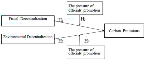
Figure 2.
The theoretical model of this paper.
3. Research Design
3.1. Econometric Model Setting
The traditional static panel data econometric model has some defects in the study of carbon emissions, as it mainly ignores the path dependence of carbon emissions and lacks consideration of the spatial spillover effect of carbon emissions [39]. This research follows the ideas of Sigman [16] and He [23] on the relationship model between decentralization system and environmental quality. Given the spatial spillover effect of carbon emissions due to air flow, the spatial lag term of carbon emissions was added into the model. Meanwhile, as there is a certain path dependence of carbon emissions, in order to avoid the problem of estimation bias due to omitted variables and the potential endogeneity problem, a further time-lagged term of carbon emissions is added to the model, thus constituting a dynamic spatial panel data model. There are three basic forms of spatial econometric models: the spatial lag model (SAR), the spatial error model (SEM) and the spatial Durbin model (SDM). Among them, the spatial Durbin model takes into account the spatial correlation between the dependent variable and the independent variable, which enables the analysis of both the influence of the independent variable on the dependent variable in the region and the influence of the dependent variable on the independent variable and the dependent variable in neighbouring regions. Therefore, this paper chooses to construct a dynamic panel data spatial Durbin model to test the relationship among fiscal decentralization, environmental decentralization and carbon emissions. To test H1 and H2, the models are set up as follows:
where: i and t represent region and year, respectively. lnco2it represents the carbon emissions per capita in province i in year t. fdit represents the level of fiscal decentralization. edit represents the level of environmental decentralization. Xit represents other control variables that affect the level of carbon emissions. W is the spatial weight matrix and εit is the random error term. ∂, ρ, α, β, γ and κ are parameters to be estimated. The control variables are mainly selected from environmental regulation, technological progress, foreign direct investment and industrial structure.
To test H3 and H4, we add the intersection terms of fiscal decentralization and official promotion pressure, environmental decentralization and official promotion pressure in models (1)–(3) above respectively to test the moderating effect of local officials’ promotion pressure, and construct the following data models, respectively:
In Models (4)–(6), pressureit is the officials’ promotion pressure index. The remaining variables are the same as in Models (1)–(3).
3.2. Data Sources and Selection of Variables
3.2.1. Data Sources
Due to the availability of data, this paper selects panel data from 30 provincial-level administrative regions in Mainland China from 2006 to 2016 (Tibet is excluded due to some missing data) for empirical analysis. The fossil energy consumption data involved in the carbon emission calculation are derived from the regional energy balance table in China’s Energy Statistical Yearbook, and the cement production data was taken from the CSMAR database. The officials’ promotion pressure indicator came from the database of China’s leading cadres, China’s political database, and the database of the local authorities. The remaining variables were obtained from the Chinese Statistical Yearbook, the Chinese Environmental Yearbook, the Chinese Environmental Statistical Yearbook and the Chinese Statistical Yearbook of Science and Technology. All monetary unit indicators are deflated using 2006 as the base period price.
3.2.2. Selection of Variables
Explained Variable
Carbon emission level lnco2. Carbon emissions are mainly derived from fossil fuel combustion and cement production activities. In this paper, the IPCC default method was used to calculate the carbon emissions, and the carbon emission coefficient was calculated according to the IPCC “Guidelines for National Greenhouse Gas Emission Inventory”. Here, the carbon emissions of each region are divided by the local GDP and then the logarithm is taken to calculate the carbon emission intensity index, which is used as the explained variable of the model.
Explanatory Variables
- Fiscal decentralization fd
Referencing the method of You and Zhang [40], this paper defined fiscal decentralization as the share of a region’s fiscal expenditure in the total fiscal expenditure. Higher fiscal decentralization values indicate a higher degree of decentralization, which means that local governments have more discretion in the allocation of public expenditure within their jurisdictions. In order to avoid the problem of multicollinearity, while at the same time removing the influence of demographic factors on the scale of fiscal expenditure, the fiscal expenditure indicators are per capitaized.
- Environmental decentralization ed
The essence of environmental decentralization is the allocation of authority for environmental affairs management. Changes in the scale and proportion of central and local environmental protection organizations and personnel can reflect the variation of the environmental management system. Based on the methods of Yu et al. [41] and Ran et al. [38], this paper measures the degree of environmental decentralization by the ratio of the per capita environmental protection staff in the region to that of whole nation. A higher degree of environmental decentralization indicates that the local government has greater authority over environmental management within its jurisdiction.
Moderating Variable
Officials’ promotion pressure (pressure). Generally, local officials judge the level of promotion pressure based on the overall frequency of official turnover. This paper drew on the research methods of Wang and Xu [42] and constructed an official promotion pressure index. By first calculating the total annual turnover of local officials (provincial governors and provincial party secretaries) in a region; Secondly, the intermediate variable for a province in given year is calculated as the sum of the number of provincial officials’ turnover in that year minus the number of turnover of officials in the province itself. Then the intermediate variables constructed above are normalized. Finally, the sum of the standardized intermediate variables for each province is subtracted from the standardized intermediate variables for that region and then divided by the number of provinces and districts to obtain the final variable.
Control Variables
In order to control for the influence of other factors on carbon emissions, the following control variables are introduced:
- Environmental regulation (er). Common indicators of environmental regulation include sewage charges, the proportion of GDP spent on environmental pollution control, and the number of environmental regulations [43,44,45]. In the past three decades, the sewage charging system in China has played an irreplaceable role in curbing environmental pollution, thus the logarithm of per capita sewage charge income was used as a proxy variable for environmental regulation in this paper.
- Technology innovation (tech). Technological innovation is the inexhaustible driving force of economic development. Technological innovation can be to improve production efficiency, expand the scale of production. It can also be about improving ecological technology, achieving cleaner production and reducing pollutant emissions. This paper measured the degree of technological innovation by the proportion of internal expenditure of R&D to GDP.
- Foreign direct investment (fdi). Each local government may lower the environmental access threshold to attract more foreign investment, thus exacerbating the region’s carbon emissions; or it may acquire more advanced clean production technologies through the introduction of foreign direct investment, thus creating a positive and good demonstration effect for economic development. In this paper, the logarithm of the amount of foreign direct investment was used to measure the level of foreign investment utilized in each province, and the annual average exchange rate of RMB to USD is used to convert to RMB.
- Industrial structure (is). The changes in industrial structure can affect regional carbon emissions. Heavy industry and construction in the secondary sector are the main sources of carbon emissions, while the tertiary sector is mostly a low-pollution emission industry, thus the higher the proportion of the tertiary sector, the smaller the impact on carbon emissions is believed to be. This paper used the share of tertiary industry output in GDP to measure industrial structure.
In order to reduce the problem of possible heteroskedasticity in the model, each variable was logarithmically treated, except for values taken as ratios or standardized values, and the calculation methods and descriptive statistical characteristics of each variable are shown in Table 1.

Table 1.
Calculation method and descriptive statistics for each variable.
3.3. Correlation Coefficient Matrix Analysis of the Main Explanatory Variables
In order to test whether there is a correlation problem between the explanatory variables of the econometric model, the correlation coefficients of the main variables are reported as shown in Table 2.
Table 2.
Correlation coefficient matrix of the main explanatory variables.
The table above shows that the correlation coefficients between the explanatory variables are very low. A separate variance inflation factor (VIF) analysis was also carried out in this paper, and the calculated results show that the mean VIF value is 1.78 and the maximum value is 3.11, which is much lower than the empirical standard value of 10, indicating that there is no multicollinearity between the variables.
3.4. Analysis on the Level of Fiscal Decentralization and Environmental Decentralization
The average levels of fiscal decentralization and environmental decentralization by region at 2006–2016 are shown in Figure 3, from which it can be seen that there are significant differences between the two, with the top three regions in terms of fiscal decentralization being Shanghai, Beijing and Tianjin, all in the developed eastern region, and the overall level of decentralization being highest in the eastern coastal region, followed by the central region and lowest in the western region. Meanwhile, the top three regions in terms of environmental decentralization are Shanxi, Henan and Hebei, all of which are located in the central and western regions. Since fiscal decentralization and environmental decentralization exist simultaneously in China without being substituted for each other, the two must be considered together in order to prevent biased results due to variable bias.
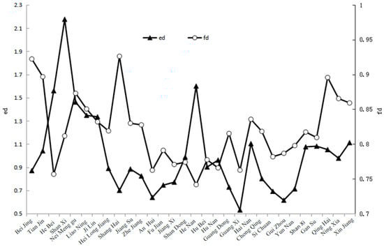
Figure 3.
The levels of fiscal decentralization (fd) and environmental decentralization (ed) by region.
4. Empirical Results and Analysis
4.1. Spatial Correlation Test
“The First Law of Geography” states that “everything is related to everything else, but things closer together are more related than things farther away”, so we have to consider the spatial correlation among regions when studying carbon emissions. There are various ways of selecting the spatial weight matrix, such as geographical proximity, geographical distance and economic distance. Generally speaking, neighbouring regions are more closely related to each other, so this paper used the adjacent weight matrix (W-01) for empirical analysis, it means that wij = 1 if there is a common boundary between two regions, and wij = 0 if not.
The existence of spatial correlation in the model can be tested by Moran’s I index. The spatial weight matrix was normalized in this paper, so that the Moran’s index formula chosen is:
where wij is the spatial weight matrix. n is the number of regions. is the observed value of the region i. is the mean of the study variables. Moran’s I index takes values between −1 and 1, with values greater than 0 indicating that economic indicators are spatially positively correlated, equal to 0 indicating that they are spatially uncorrelated, and less than 0 indicating that they are spatially negatively correlated. Table 3 presents the Moran’s I index for carbon emissions over the sample period. From the table, the Moran index is greater than 0 for all years during the period 2006–2016, and all are significant at the 1% probability level, indicating that carbon emissions in each region exhibit a significant positive spatial correlation.
Table 3.
Regional Moran’s I index of carbon emissions (2006–2016).
4.2. Analysis of Basic Regression Results
In this paper, the Stata 15.0 software was used to make regression for the econometric models (1–6), and the specific regression results were shown in Table 4. In order to test whether the spatial Durbin model would degenerate into a spatial lag model or a spatial error model, LR test and LM test were used to make the decision respectively. The test results show that the LR_spatial_lag, LR_spatial_error, LM_spatial_lag and LM_spatial_error values of all models reject the original hypothesis at the 5% level, it indicates that the spatial Durbin model is appropriate. In addition, the results of Hausman test indicated that the fixed effect models were applied to all six models. The regression results show that the coefficients of the one-period time-lagged term of the carbon emissions (L.lnco2) are all significantly positively correlated at the 1% level, indicating that there is significant continuity and stickiness in carbon emissions, and that current carbon emissions are susceptible to the effects of the previous period. The estimated coefficients of the spatial lagged term (Wlnco2) of carbon emissions are also significantly positive at the 1% level, indicating that carbon emissions among provinces show significant spatial dependence, an increase in carbon emissions in neighbouring regions will aggravate carbon emissions in the region.
Table 4.
Basic regression results for fiscal decentralization, environmental decentralization, officials’ promotion pressure and carbon emissions.
4.2.1. Analysis of the Main Effects of Fiscal Decentralization and Environmental Decentralization on Carbon Emissions
The results of the dynamic panel data space Durbin model estimation with fiscal decentralization as the explanatory variable are reported in Model 1 in Table 4. From the model estimates, the coefficient of fd is 0.585, which is significantly positive at the 5% level, indicating that fiscal decentralization increases carbon emissions in the region, supporting the “race to bottom” view. The coefficient of the variable related to spatial weighting Wfd is 0.392, which is significant at the 5% level, indicating that a 1% increase in fiscal decentralization in the neighbouring region increases the carbon emissions level in the region by 0.392%. From the above results, it can be seen that hypothesis H1 is fully valid. Fiscal decentralization exacerbates carbon emissions in the region, and fiscal decentralization in neighbouring regions has a significant exacerbating effect on carbon emissions in the region. This shows that when the fiscal decentralization of neighbouring regions increases, the local government will adopt a similar competitive strategy by lowering environmental standards to attract high-emission and high-tax enterprises to locate in their jurisdictions, thus increasing the carbon emissions of the region.
The regression results of the effect of environmental decentralization on carbon intensity are reported in Model 2 in Table 4. A significant negative coefficient is estimated for ed in the regression results. This indicates that the current environmental decentralization system in China has played a positive role in curbing carbon emissions. However, the coefficient of Wed is significantly positive. That is, an increase in the level of environmental decentralization in neighbouring regions will exacerbate carbon emissions in the region, so the regression results are not entirely consistent with hypothesis H2. The likely reason is that while the environmental decentralization system is effective in curbing carbon emissions in the region, the competition among local governments adopts a differentiated competition strategy. That is, when neighbouring regions increase the level of environmental decentralization and strengthen environmental regulation, the local region adopts the opposite strategy, leading to the relocation of high carbon emitting enterprises from the neighbouring region to the region, which in turn leads to an increase in carbon emissions in the region.
Model 3 in Table 4 reports the results of both fiscal decentralization and environmental decentralization on carbon emissions intensity. The regression results show a significant positive relationship between fiscal fd and carbon emissions. In contrast, there is a significant negative relationship between ed and carbon emissions, in line with the previous findings of Model 1 and Model 2. This shows that fiscal decentralization focuses on stimulating regional economic development, while environmental decentralization endures local authority to protect and control the environment, thus making it possible for fiscal decentralization to increase carbon emissions while environmental decentralization suppresses them. Significantly, the coefficient of the intersection term fd × ed is significantly negative at the 1% probability level, it indicates that as the country gradually pays more attention to carbon emission reduction governance, the contribution of environmental decentralization to carbon emission reduction begins to exceed the exacerbating effect of fiscal decentralization. Therefore, the comprehensive effect on carbon emission reduction is significant.
4.2.2. Analysis of the Moderating Effect of Officials’ Promotion Pressure in the Impact of Fiscal Decentralization and Environmental Decentralization on Carbon Emissions
In Table 4, the analysis results of the main effects of fiscal decentralization and environmental decentralization on carbon emissions in Model 4–6 are basically consistent with Model 1–3 except for slight differences in coefficient values and significance. The moderating effect of officials’ promotion pressure is mainly analyzed here. The coefficient of the intersection term fd × pressure in Model 4 is 1.007 and is significantly positive at the 5% probability level. This indicates that the variable of officials’ promotion pressure has a positive moderating effect on the effect of fiscal decentralization on carbon emissions, and fully supports hypothesis H3. Under the premise that the central government increases environmental responsibilities of local governments, local governments will consider the ecological impact, and thus the economic competition incentive decreases and the ecological environment pressure gradually increases. Nonetheless, economic promotion still takes precedence, and local officials make decisions to maximize economic efficiency within the boundaries of the green performance assessment under the fiscal decentralization system.
The coefficient of the intersection term ed×pressure in Model 5 is significantly positive at the 5% probability level. This indicates that although a purely environmental decentralization system is effective in curbing carbon emission levels, the promotion pressure on local officials can alter the curbing effect. The combination of the two exacerbates carbon emissions, which is fully consistent with Hypothesis H4. Since carbon emissions have strong negative spatial externality, it leads to a mismatch between the benefits and costs of its management. Hence, local officials are more willing to “free ride” on policy.
The coefficient of the intersection term fd × ed × pressure in Model 6 is significantly positive at the 1% probability level. This indicates that officials’ promotion pressure plays a positive moderating role in the impact of the decentralization system on carbon emissions. As the competition for local officials becomes more intense, the negative impact of the combined effect of environmental decentralization and fiscal decentralization and official promotion pressure on curbing carbon emissions will be further exacerbated.
4.2.3. Analysis of Other Effects
As for the estimation results of control variables, the direction and significance of the coefficient of variables in each model are basically the same. The coefficient on the environmental regulation variable (er) is significantly positive, which is the exact opposite of what would be expected conventionally. The likely reason is that the emission charge system has a very weak inhibiting effect on carbon emissions due to the interference of human factors, and there is even a “green paradox” phenomenon that the more charges the more carbon emissions. In order to solve the problems of insufficient enforcement rigidity and local government intervention in the emission charging system, China has introduced the new “Environmental Protection Tax Law” since 1 January 2018, which ensures the legalization and standardization of environmental protection charges and is more conducive to the promotion of carbon emission reduction.
The coefficient of tech is significantly negative, it shows that the current technological progress has a certain promotion effect on curbing carbon emissions, but the coefficient is very small, indicating that the overall effectiveness still needs to be improved. The state should increase its investment in eco-technology innovation, guide and support production enterprises to carry out eco-technology innovation in energy saving and emission reduction.
The significant positive coefficient of fdi suggests that local governments may have lowered the environmental access threshold to attract more foreign investment, thus exacerbating carbon emissions in the region. The local governments should be strict in introducing foreign investment and introduce as many energy-saving, emission-reducing and clean production projects as possible.
The coefficient of is is significantly negative, which implies that a higher proportion of value added in the tertiary sector can better reduce carbon emissions. The government should also continue to practice industrial restructuring, pushing enterprises to transform their structures, increase the proportion of tertiary industries, and develop the industrial structure towards advanced levels, so as to achieve a win-win situation for both economic and ecological benefits.
4.3. Regional Analysis
The level of economic development and technological progress, natural resource endowment, industrial structure and the level of foreign investment introduced vary greatly from region to region. Therefore, the level of decentralization is also heterogeneous, which leads to a different impact of decentralization on carbon emissions in different regions. Consequently, it is necessary to analyze the impact of decentralization systems on carbon emissions differently by region. This paper divides the 30 provinces into 3 regions according to the general division of the National Statistical Bureau: the eastern region includes Beijing, Tianjin, Hebei, Liaoning, Shanghai, Jiangsu, Zhejiang, Fujian, Shandong, Guangdong and Hainan; the central region includes Shanxi, Jilin, Heilongjiang, Anhui, Jiangxi, Henan, Hubei and Hunan, and the rest of the provinces belong to the western region. The regression analysis was carried out separately for model (6). The results are presented in Appendix A, where columns (1–3) used the adjacent weight matrix(W-01). Columns (4–6) use the economic distance weight matrix(W-ed) for stability testing of the sub-regional analysis. The economic distance weight matrix formula is as follows:
where indicates the GDP per capita of region i.
Appendix A shows that the coefficients of L.lnco2 and Wlnco2 in all regions are significantly positive, regardless of geographical proximity or economic distance. This indicates that carbon emissions show a strong path dependence in both space and time. Overall, the coefficients of fiscal decentralization in the East, Central and Western regions are all significantly positive. The most significant difference between the three areas is the difference in environmental decentralization indicators. Whereas environmental decentralization in the eastern region is better at curbing carbon emissions, the opposite is true in the western region, while it is not significant in the central region. Looking at the intersection term fd × ed, whereas in the eastern region the higher the degree of decentralization, the lower the level of carbon emissions, in the central and western regions the combined degree of decentralization is negatively, but insignificantly, related to the level of carbon emissions. When the moderating variable of local officials’ promotion pressure is added, the intersection term of the three variables fd × ed × pressure has a negative though insignificant coefficient in the eastern and central regions, this indicates that although the intense promotion pressure of local officials can lead to weaker implementation of carbon reduction policies, the overall policy still has a dampening effect on carbon emissions. Nevertheless, the coefficient remains significantly positive in the western region.
4.4. Stability Tests
In order to mitigate the impact of the indicator metric problem on the empirical results, the following different methods were used to test the stability of the empirical findings of the regression model (6) respectively, and the specific stability test results are shown in Appendix B.
(1) The use of a per capita carbon emissions indicator. The carbon emissions indicator can be divided into “total” and “intensity” indicators. The carbon intensity indicator was used in the basic regression analysis. Here, the logarithm of per capita carbon emissions is used to represent the total amount of carbon emissions to replace the dependent variable carbon emission intensity for stability test. The estimated results are shown in column (1) of Appendix B.
(2) The use of economic distance weight matrix. Carbon emissions are mainly caused by industrial production, the economic distance is introduced into the spatial weight matrix in order to better fit the regional economic development, and meanwhile to check whether the basic regression results are sensitive to the spatial weight. The specific stability test results are shown in column (2).
(3) The use of adjusted environmental decentralization indicators. The environmental decentralization variables may be affected by the size of GDP and thus cause endogenous disturbances, therefore we obtain the adjusted environmental decentralization indicator (aedit) by multiplying the above environmental weighting indicator by a GDP reduction factor, as shown in Equation (9):
where (1 − gdpit/gdpt) is the economic size reduction factor, gdpit is the GDP of province i in year t, and gdpt is the GDP in year t. The specific regression results are shown in column (3).
(4) The use of lagged one-period indicators for the environmental decentralization and fiscal decentralization and official promotion pressure variables. In order to examine the existence of endogeneity between carbon emission intensity and environmental decentralization and fiscal decentralization, we will use lagged endogenous variables for stability testing. The lagged one-periods of the three main explanatory variables of environmental decentralization, fiscal decentralization and officials’ promotion pressure are regressed in place of the original corresponding explanatory variables. The specific regression results are shown in column (4).
The results show that the coefficients of the variables are basically consistent with Table 4 in terms of direction and significance, indicating that the regression model is highly robust.
5. Discussion
This paper begins by the analyzing the impacts of fiscal decentralization and environmental decentralization on China’s carbon emissions, and then introduced the promotion pressure of local officials as the main factor and discusses its moderating effect on decentralization system and carbon emissions. The empirical results provide strong support for our previous research hypothesis and generate important theoretical and managerial implications.
5.1. Policy Implications
The policy implications in this study are as follows:
First, China’s carbon emissions show obvious spatial spillover and a time-dependent path, so the government needs to implement top-level designs from a strategic perspective in order to deal with this problem. The central government can establish a cross-regional cooperation system and a pollution compensation mechanism [38], joint prevention and governance should be carried out in space and sustained in time. In addition to considering the carbon emissions of the region itself, it should also comprehensively take the carbon emissions of neighboring regions into consideration, strengthen the active cooperation between regions [3], and ensure the continuous and steady progress of carbon emission reduction work.
Second, fiscal decentralization is a very important system. Although fiscal decentralization has a positive correlation with carbon emissions, it does not imply China’s fiscal decentralization system should be denied, but rather the existing decentralization system should be improved further [46]. Investments in major infrastructure projects involving environmental protection and welfare should be relatively centralized and deployed by the central government [47], which can significantly reduce cross-border pollution and free-riding problems.
Third, the environmental decentralization system is effective for carbon emission reduction. It is an interesting study on how to determine a reasonable level of environmental decentralization and give better play to the central and local governments to improve the efficiency of carbon emission control. There is a strong heterogeneity in carbon emissions among different regions in China, the local governments are more aware of the economic development and ecological and environmental conditions within their jurisdictions than the central government, and are able to deal with and rectify environmental problems in a more timely and convenient manner. Meanwhile, the responsibilities and powers of local environmental protection departments should be strengthened to take on the task of monitoring, testing and supervising the improvement of the ecological environment [27,48].
Fourth, the implementation capacity of local governments’ carbon emission reduction work is a key issue that cannot be ignored. The system for evaluating the performance of local officials needs to be improved, it is necessary to quantify and integrate their performance in energy conservation and emission reduction, and introduce a third-party evaluation system to guide local officials to compete in a healthy way [48]. Considering the heterogeneity of regional development, the assessment system of local officials should be improved in a gradient. In economically developed regions and environmentally fragile regions, the proportion of fiscal assessment and GDP assessment should be moderately reduced. Increase the incentive of ecological performance assessment to motivate local officials’ policy implementation, Reversing the competition for local officials from “race to the bottom” of environment to “race to the top”, “competition of ecological performance” and the competition of “harmony between human beings and nature” [10].
Fifth, the impacts of decentralization on carbon emissions are different in the eastern, central and western regions. The high level of economic development in the east, especially in the coastal areas, which naturally places higher demands on the ecological environment than other regions. Moreover, the economic structure is dominated by the third sector, and local governments have no incentive or possibility to trade the environment for economic growth, so the eastern region has taken the lead in realizing a virtuous circle of economic growth and environmental protection. In the central region, which is currently in a stage of economic emergence, economic development and environmental protection are beginning to show a more harmonious trend after a long period of conflict, but the effect of low-carbon development is not obvious. The central region needs to be strictly monitored and guided by the state while encouraging it to strengthen its economic construction. At present, the western region is still relatively backward, developing economy to solve the problems of people’s livelihood is the top priority. The local governments may sacrifice the environment to some extent in exchange for economic growth. In addition, the rich resources and fragile ecological base of the western region will make it more risky to trade the environment for growth. Therefore, it is essential to implement differentiated strategies, taking into account the comparative advantages of the regions according to local conditions.
5.2. Contributions of This Article
The following contributions were provided by this article:
First, based on the particularity and complexity of Chinese style decentralization system, it measures the effect of the fiscal decentralization and environmental decentralization on carbon emissions and analyzes the interactions of these two decentralization systems, which avoids errors in the variable measurement.
Second, from the perspective of the influence of local officials’ behavior on the decentralization system under the promotion pressure, it analyzes the moderating role of local officials’ promotion pressure on the impact of fiscal decentralization and environmental decentralization on carbon emissions, which broadens the research field of carbon emissions.
Third, according to spatial Durbin model (SDM) of dynamic panel data, with fully consideration of the path dependence and spatial spillover of carbon emissions, it not only analyzes the spatial effect of carbon emissions, but also deeply studies the impact of decentralization policy in adjacent jurisdictions on carbon emissions of one region, enriching the research of carbon emissions.
Fourth, it conducts regional analysis of the effect of decentralization system on carbon emission, which provides a reference for the eastern, central and western regions to adopt differentiated strategies for carbon emission reduction.
5.3. Method Limitations
First, due to limited data being available, this article discussed the effect of decentralized system on carbon emissions only from the provincial level, but each province in China has a large area, there will also be heterogeneity between cities within the province. Therefore, future research will focus on in-depth studies at the city level to make a more accurate analysis of the impact of decentralization on carbon emissions and the behavioral orientation of local officials under the pressure of promotion.
Second, the time span of this study is limited from 2006 to 2016, but the decentralization system and the assessment criteria for local officials in China are in dynamic change. If the time dimension is extended, the impact of decentralization system on carbon emissions may be different, and we will continue to pay attention to this problem in the future.
Third, the index measurement methods in this study are not rich enough, more comprehensive index measurement will be conducted in future study. For example, the fiscal decentralization index may be measured from other perspectives, and the environmental decentralization can be subdivided into three dimensions of environmental administrative decentralization, environmental supervision decentralization and environmental monitoring decentralization for in-depth analysis.
6. Conclusions
This article used the panel data of 30 provincial-level administrative regions in Mainland China (excluding Tibet) from 2006–2016 to conduct an empirical study, using a spatial Durbin model to analyze the spatial impact of fiscal decentralization and environmental decentralization on regional carbon emissions based on the perspective of officials’ promotion pressure. Combined with the analysis of research hypothesis and empirical research results, the empirical study concludes are as follows:
First, the fiscal decentralization system exacerbates carbon emissions in the region, while increased fiscal decentralization in neighbouring regions will also increase carbon emissions in the region, the competition among local governments adopts the competition strategy of mutual imitation, and the competition between regions tends to a “race to bottom”, leading to an increase in carbon emissions rather than a decrease.
Second, unlike fiscal decentralization, the environmental decentralization is effective in curbing carbon emissions, while environmental decentralization in neighbouring regions exacerbates carbon emissions in the region. The competition between regions in the context of environmental decentralization is a “race to top”.
Third, the promotion pressure of officials plays a positive role in moderating the impact of fiscal decentralization on carbon emissions, and at the same time weakens the suppression of carbon emissions by environmental decentralization. More attention should be paid to the implementation of the responsibility of local officials for environmental policies.
Fourth, from a sub-regional perspective, fiscal decentralization is significantly and positively correlated with carbon emissions in all regions. However, the level of environmental decentralization is highly spatially heterogeneous, environmental decentralization in the eastern region effectively curbs carbon emissions, but the opposite is true in the western region, while it is not significant in the central region.
Author Contributions
All authors contributed to this work, discussed the results and implications and commented on the manuscript at all stages. Z.T. gave valuable advice on the establishment of the framework, as well as the design process. S.X. collected and analyzed data. D.Y. and S.X. discussed the main idea behind the work and reviewed and revised the manuscript. B.Y. enhanced the quality of the manuscript at all stages. All authors have read and agreed to the published version of the manuscript.
Funding
This research was funded by The National Natural Science Foundation of China, grant number 71974209 and 71573283; Major Strategic Consulting Project of Chinese Academy of Engineering, grant number 2019NXZD4; Transport Department of Hunan Province Technology Innovation Project, grant number 202037, and Hunan Provincial Education Department Project, grant number 19B177.
Conflicts of Interest
The authors declare no conflict of interest.
Appendix A
Table A1.
Regression estimates of fiscal and environmental decentralization and carbon emissions by region.
Table A1.
Regression estimates of fiscal and environmental decentralization and carbon emissions by region.
| Explanatory Variables | Ln(co2/gdp) | |||||
|---|---|---|---|---|---|---|
| Eastern | Central | Western | Eastern | Central | Western | |
| W | W-01 | W-ed | ||||
| L.lnco2 | 1.291 *** | 0.988 *** | 1.404 *** | 1.092 *** | 0.829 *** | 1.196 *** |
| (19.19) | (15.39) | (20.40) | (16.11) | (10.48) | (17.37) | |
| fd | 2.470 *** | 1.529 ** | 1.598** | 2.165 *** | 1.391** | 3.543 *** |
| (3.99) | (2.05) | (2.22) | (3.63) | (1.97) | (4.58) | |
| ed | −2.380 *** | 0.252 | 2.954 *** | −2.060 *** | −0.002 | 2.267** |
| (−3.91) | (0.37) | (3.46) | (−3.36) | (−0.00) | (2.37) | |
| er | 0.163 *** | 0.080 * | 0.189 *** | 0.155 *** | 0.018 | −0.053 |
| (4.62) | (1.70) | (5.70) | (3.91) | (0.41) | (−1.56) | |
| tech | −0.023 *** | 0.066 ** | 0.167 *** | −0.021 *** | 0.075 *** | 0.032 |
| (−2.91) | (2.55) | (8.27) | (−2.79) | (2.64) | (1.48) | |
| fdi | 0.056 *** | 0.035 | 0.004 | 0.044 *** | −0.011 | −0.011 |
| (3.19) | (1.35) | (0.38) | (2.59) | (−0.41) | (−0.89) | |
| is | −1.343 *** | −0.576 * | −2.242 *** | −1.052 *** | −0.138 | −0.695 ** |
| (−5.70) | (−1.86) | (−9.07) | (−4.62) | (−0.48) | (−2.33) | |
| fd × pressure | 3.011 *** | 2.018 ** | 2.368 *** | 2.811 *** | 1.887 ** | 4.078 *** |
| (4.37) | (2.46) | (2.95) | (4.07) | (2.08) | (5.45) | |
| ed × pressure | 2.001 ** | −0.531 | 4.282 ** | 1.902 * | 0.567 | 8.856 *** |
| (1.99) | (−0.34) | (2.31) | (1.76) | (0.34) | (3.80) | |
| fd × ed | −2.927 *** | −0.377 | −1.492 * | −2.238 *** | −0.054 | −0.899 |
| (−3.79) | (−0.45) | (−1.66) | (−2.96) | (−0.06) | (−0.84) | |
| fd × ed × pressure | −1.145 | −1.278 | 5.146 ** | −1.007 | −0.017 | 5.743 ** |
| (−0.78) | (−0.66) | (2.22) | (−0.70) | (−0.01) | (2.31) | |
| Wlnco2 | 0.152 ** | 0.114 | 1.221 *** | 0.141 ** | 0.039 | 0.064 |
| (2.14) | (1.13) | (14.15) | (1.97) | (0.36) | (0.63) | |
| Wfd | 2.052 *** | 0.811 | 7.565 *** | 1.858 *** | 1.400 * | 7.294 *** |
| (4.22) | (0.84) | (10.05) | (3.88) | (1.85) | (7.90) | |
| Wed | −0.063 | −0.139 | −1.439 ** | −0.056 | 0.453 * | −6.741 *** |
| (−0.44) | (−0.48) | (−2.21) | (−0.41) | (1.83) | (−9.48) | |
| W(fd × pressure) | −0.013 * | −0.009 | −0.070 *** | −0.010 * | −0.005 | −0.156 *** |
| (−1.70) | (−0.69) | (−5.06) | (−1.65) | (−0.41) | (−7.94) | |
| W(ed × pressure) | −0.404 | 0.864 | 6.336 *** | −0.359 | −0.139 | 17.648 *** |
| (−1.34) | (1.54) | (7.69) | (−1.18) | (−0.35) | (10.77) | |
| LR_spatial_lag | 31.57 *** | 12.23 *** | 4.31 ** | 27.17 *** | 15.30 *** | 4.55 ** |
| LR_spatial_error | 46.55 *** | 6.34 ** | 18.40 *** | 44.09 *** | 6.82 ** | 19.19 *** |
| LM_spatial_lag | 4.411 ** | 6.318 ** | 5.736 ** | 3.661 * | 7.399 ** | 6.476 ** |
| LM_spatial_error | 6.170 ** | 10.263 *** | 7.256 ** | 6.321 ** | 13.463 *** | 7.687 ** |
| N | 110 | 80 | 110 | 110 | 80 | 110 |
| Hausman test | FE | FE | FE | FE | FE | FE |
| R2 | 0.927 | 0.972 | 0.925 | 0.912 | 0.816 | 0.954 |
Notes: (1) t-values in parentheses; (2) ***, **, * denote significant at the 1%, 5% and 10% levels respectively; (3) Constant term estimates not reported; (4) Hausman test used to test for random versus fixed effects, when p > 0.05 indicates rejection of random effects in favour of fixed effects, the same as in Appendix B.
Appendix B
Table A2.
Robustness testing of different measurement indicators.
Table A2.
Robustness testing of different measurement indicators.
| Explanatory Variables | co2 | |||
|---|---|---|---|---|
| (1) | (2) | (3) | (4) | |
| L.lnco2 | 0.682 *** | 0.839 *** | 0.753 *** | 0.765 *** |
| (21.90) | (24.88) | (22.90) | (23.08) | |
| fd | 0.761 *** | 0.521 ** | 0.535 ** | 0.577 ** |
| (2.80) | (1.97) | (2.07) | (2.12) | |
| ed | −0.953 *** | −0.726 ** | −0.771 ** | −0.734 ** |
| (−2.64) | (−2.06) | (−2.33) | (−2.25) | |
| er | 0.048 *** | 0.034 ** | 0.029 ** | 0.020 |
| (3.28) | (2.50) | (2.23) | (1.61) | |
| tech | −0.000 | 0.003 | 0.002 | −0.015 * |
| (−0.03) | (0.28) | (0.23) | (−1.78) | |
| fdi | 0.023 * | 0.001 | 0.003 | −0.000 |
| (1.72) | (0.13) | (0.32) | (−0.01) | |
| is | −0.392 *** | −0.205 * | −0.284 * | −0.403 *** |
| (−2.83) | (−1.67) | (−1.94) | (−2.90) | |
| fd × pressure | 1.605 *** | 0.821 * | 0.613 | 1.337 ** |
| (2.77) | (1.68) | (1.02) | (2.04) | |
| ed × pressure | 1.814 ** | 1.038 | 1.214 * | 1.344 * |
| (2.30) | (1.31) | (1.65) | (1.76) | |
| fd × ed | −1.138 ** | −0.798 * | −0.828 * | −0.434 ** |
| (−2.46) | (−1.78) | (−1.95) | (−2.01) | |
| fd × ed × pressure | −2.185 ** | −1.112 | −1.295 | −0.501 |
| (−2.09) | (−1.08) | (−1.34) | (−0.72) | |
| Wlnco2 | 0.203 *** | 0.171 *** | 0.288 *** | 0.295 *** |
| (4.08) | (3.64) | (5.97) | (6.90) | |
| Wfd | 1.019 *** | 0.213 | 0.752 ** | 0.667 * |
| (2.96) | (0.47) | (2.09) | (1.64) | |
| Wed | 0.348 *** | 0.277 ** | 0.272 ** | 0.185 * |
| (3.05) | (2.07) | (2.23) | (1.75) | |
| W(fd × pressure) | −0.305 | −1.199 * | −0.275 | −1.364 ** |
| (−0.59) | (−1.75) | (−0.37) | (−2.39) | |
| W(ed × pressure) | 0.027 | 0.948 * | −0.132 | 1.305 ** |
| (0.08) | (1.66) | (−0.42) | (2.17) | |
| LR_spatial_lag | 15.72 *** | 11.59 *** | 17.97 ** | 31.98 *** |
| LR_spatial_error | 27.26 *** | 14.51 *** | 37.85 *** | 62.80 *** |
| LM_spatial_lag | 8.004 *** | 4.097 ** | 5.548 ** | 5.252 ** |
| LM_spatial_error | 22.172 *** | 14.638 *** | 12.243 *** | 11.513 *** |
| N | 330 | 330 | 330 | 330 |
| Hausman test | FE | FE | FE | FE |
| R2 | 0.960 | 0.980 | 0.945 | 0.956 |
***, **, * denote significant at the 1%, 5% and 10% levels respectively.
References
- Global Carbon Atlas. CO2 Emissions Data. Available online: http://www.globalcarbonatlas.org/en/CO2-emissions (accessed on 4 October 2020).
- Song, M.; Du, J.; Tan, K.H. Impact of fiscal decentralization on green total factor productivity. Int. J. Prod. Econ. 2018, 205, 359–367. [Google Scholar] [CrossRef]
- Shi, L.; Yang, F.; Gao, L. The Allocation of Carbon Intensity Reduction Target by 2030 among Cities in China. Energies 2020, 13, 6006. [Google Scholar] [CrossRef]
- Konisky, D.M. Regulatory Competition and Environmental Enforcement: Is There a Race to the Bottom? Am. J. Polit. Sci. 2007, 51, 853–872. [Google Scholar] [CrossRef]
- Yao, X.; Zhou, H.; Zhang, A.; Li, A. Regional energy efficiency, carbon emission performance and technology gaps in China: A meta-frontier non-radial directional distance function analysis. Energy Policy 2015, 84, 142–154. [Google Scholar] [CrossRef]
- Mi, Z.F.; Pan, S.Y.; Yu, H.; Wei, Y.M. Potential impacts of industrial structure on energy consumption and CO2 emission: A case study of Beijing. J. Clean. Prod. 2015, 103, 455–462. [Google Scholar] [CrossRef]
- Shahzad, S.J.H.; Kumar, R.R.; Zakaria, M.; Hurr, M. Carbon emission, energy consumption, trade openness and financial development in Pakistan: A revisit. Renew. Sustain. Energy Rev. 2017, 70, 185–192. [Google Scholar] [CrossRef]
- Shen, L.; Wu, Y.; Lou, Y.; Zeng, D.; Shuai, C.; Song, X. What drives the carbon emission in the Chinese cities?—A case of pilot low carbon city of Beijing. J. Clean. Prod. 2018, 174, 343–354. [Google Scholar] [CrossRef]
- Khan, M.K.; Khan, M.I.; Rehan, M. The relationship between energy consumption, economic growth and carbon dioxide emissions in Pakistan. Financ. Innov. 2020, 6, 1–13. [Google Scholar] [CrossRef]
- Cheng, S.L.; Fan, W.; Chen, J.D.; Meng, F.X.; Liu, G.Y.; Song, M.L.; Yang, Z.F. The impact of fiscal decentralization on CO2 emissions in China. Energy 2020, 192, 1–15. [Google Scholar] [CrossRef]
- Zhu, J.; Xu, Z.W. Fiscal decentralization, regional fiscal competition and macroeconomic fluctuations in China. Econ. Res. J. 2018, 1, 21–34, (In Chinese with English abstract). [Google Scholar]
- Feng, S.; Sui, B.; Liu, H.; Li, G. Environmental decentralization and innovation in China. Econ. Model. 2020, 93, 660–674. [Google Scholar] [CrossRef]
- Qian, Y.; Weingast, R. Federalism as a commitment to preserving market incentives. J. Econ. Persp. 1997, 11, 83–92. [Google Scholar] [CrossRef]
- Gornik, V.G. Organization intergovernmental fiscal relations with principles of the theory of fiscal federalism. Management 2015, 9, 221–229. [Google Scholar]
- Kuai, P.; Yang, S.; Tao, A.; Zhang, S.; Khan, Z.D. Environmental effects of Chinese-style fiscal decentralization and the sustainability implications. J. Clean. Prod. 2019, 239, 1–13. [Google Scholar] [CrossRef]
- Sigman, H. Decentralization and Environmental Quality: An International Analysis of Water Pollution Levels and Variation. Land Econ. 2014, 90, 114–130. [Google Scholar] [CrossRef]
- Woods, N.D. Interstate Competition and Environmental Regulation: A Test of the Race-to-the-Bottom Thesis. Soc. Sci. Q. 2006, 87, 174–189. [Google Scholar] [CrossRef]
- Kang, D. Will Chinese System of Fiscal Decentralization Inhibit the Environmental Investment? Am. J. Ind. Bus. Manag. 2016, 6, 439–443. [Google Scholar] [CrossRef][Green Version]
- Zhang, K.Z.; Wang, J.; Cui, X.Y. Fiscal decentralization and environment pollution: From the perspective of carbon emission. China Ind. Econ. 2011, 10, 65–75, (In Chinese with English abstract). [Google Scholar]
- Magnani, E. The Environmental Kuznets Curve, environmental protection policy and income distribution. Ecol. Econ. 2000, 32, 431–443. [Google Scholar] [CrossRef]
- Gray, W.B.; Shadbegian, R.J. Optimal pollution abatement: Whose benefits matter, and how much? J. Environ. Econ. Manag. 2002, 47, 510–534. [Google Scholar] [CrossRef]
- List, J.A.; Gerking, S. Regulatory Federalism and Environmental Protection in the United States. J. Reg. Sci. 2000, 40, 453–471. [Google Scholar] [CrossRef]
- He, Q. Fiscal decentralization and environmental pollution: Evidence from Chinese panel data. China Econ. Rev. 2015, 36, 86–100. [Google Scholar] [CrossRef]
- Sigman, H. Transboundary spillovers and decentralization of environmental policies. J. Environ. Econ. Manag. 2005, 50, 82–101. [Google Scholar] [CrossRef]
- Tiebout, C.M. A Pure Theory of Local Expenditures. J. Polit. Econ. 1956, 64, 416–424. [Google Scholar] [CrossRef]
- Oates, W.E.; Portney, P.R. The Political Economy of Environmental Policy. In Handbook of Environmental Economics, 1st ed.; Mäler, K.G., Vincent, J.R., Eds.; Elsevier: Amsterdam, The Netherlands, 2003; Volume 1, pp. 325–354, Chapter 8. [Google Scholar]
- Millimet, D.L. Environmental Federalism: A Survey of the Empirical Literature. IZA Discussion Paper No. 7831. Available online: https://ssrn.com/abstract=2372540 (accessed on 4 October 2020).
- Banzhaf, H.S.; Chupp, H.; Harm, V.W. Spatial Spillovers: Environmental Federalism and US Air Pollution. Working Paper, NBER. 2010. Available online: https://www.nber.org/papers/w15666 (accessed on 4 October 2020).
- Levinson, A. Environmental Regulatory Competition: A Status Report and Some New Evidence. Natl. Tax J. 2003, 56, 91–106. [Google Scholar] [CrossRef]
- Oates, W.E. On the Evolution of Fiscal Federalism: Theory and Institutions. Natl. Tax J. 2008, 61, 313–334. [Google Scholar] [CrossRef]
- Malueg, D.A.; Yates, A.J. Strategic Behavior, Private Information, and Decentralization in the European Union Emissions Trading System. Environ. Resour. Econ. 2009, 43, 413–432. [Google Scholar] [CrossRef]
- Chang, H.F.; Sigman, H.; Traub, L.G. Endogenous decentralization in federal environmental policies. Int. Rev. Law Econ. 2014, 37, 39–50. [Google Scholar] [CrossRef]
- D’Amato, A.; Valentini, E. Enforcement and environmental quality in a decentralized emission trading system. J. Regul. Econ. 2011, 40, 141–159. [Google Scholar] [CrossRef]
- Zhou, C.H.; Zhang, X.M. Measuring the Efficiency of Fiscal Policies for Environmental Pollution Control and the Spatial Effect of Fiscal Decentralization in China. Int. J. Environ. Res. Public Health 2020, 17, 8974. [Google Scholar] [CrossRef]
- Zhang, K.; Zhang, Z.Y.; Liang, Q.M. An empirical analysis of the green paradox in China: From the perspective of fiscal decentralization. Energy Policy 2017, 103, 203–211. [Google Scholar] [CrossRef]
- Zhang, X. Fiscal decentralization and political centralization in China: Implications for growth and inequality. J. Comp. Econ. 2006, 34, 713–726. [Google Scholar] [CrossRef]
- Cole, M.A.; Elliott, R.J.R.; Okubo, T.; Zhou, Y. The carbon dioxide emissions of firms: A spatial analysis. J. Environ. Econ. Manag. 2013, 65, 290–309. [Google Scholar] [CrossRef]
- Ran, Q.Y.; Zhang, J.N.; Hao, Y. Does environmental decentralization exacerbate China’s carbon emissions? Evidence based on dynamic threshold effect analysis. Sci. Total Environ. 2020, 721, 137656. [Google Scholar] [CrossRef]
- Pao, H.T.; Tsai, C.M. Modeling and forecasting the CO2 emissions, energy consumption, and economic growth in Brazil. Energy 2011, 36, 2450–2458. [Google Scholar] [CrossRef]
- You, D.M.; Zhang, Y.; Yuan, B.L. Environmental regulation and firm eco-innovation: Evidence of moderating effects of fiscal decentralization and political competition from listed Chinese industrial companies. J. Clean. Prod. 2019, 207, 1072–1083. [Google Scholar] [CrossRef]
- Yu, Q.; Lu, H.Y.; Xu, Y.K. Research on reformation of China’s environment decentralization system: Institutional change, numerical estimates and effects assessment. China Ind. Econ. 2014, 1, 31–43. [Google Scholar]
- Wang, X.B.; Xu, X.X. Local offificials promoted competition and economic growth. Econ. Sci. 2010, 6, 42–58. (In Chinese) [Google Scholar]
- Fredriksson, P.G.; Millimet, D.L. Strategic Interaction and the Determination of Environmental Policy across U.S. States. J. Urban Econ. 2002, 51, 101–122. [Google Scholar] [CrossRef]
- Xie, R.H.; Yuan, Y.J.; Huang, J.J. Different Types of Environmental Regulations and Heterogeneous Influence on “Green” Productivity: Evidence from China. Ecol. Econ. 2017, 132, 104–112. [Google Scholar] [CrossRef]
- Yang, C.H.; Tseng, Y.H.; Chen, C.P. Environmental regulation, induced R&D, and productivity: Evidence from Taiwan’s manufacturing industries. Resour. Energy Econ. 2012, 34, 514–532. [Google Scholar]
- Zhang, B.; Chen, X.L.; Guo, H.X. Does central supervision enhance local environment enforcement? Quasi-experimental evidence from China. J. Public Econ. 2018, 164, 70–90. [Google Scholar] [CrossRef]
- Konisky, D.M.; Woods, N.D. Environmental Free Riding in State Water Pollution Enforcement. State Politi-Policy Q. 2012, 12, 227–251. [Google Scholar] [CrossRef]
- Wu, H.T.; Li, Y.W.; Hao, Y.; Ren, S.Y.; Zhang, P.F. Environmental decentralization, local government competition, and regional green development: Evidence from China. Sci. Total. Environ. 2020, 708, 135085. [Google Scholar] [CrossRef] [PubMed]


Publisher’s Note: MDPI stays neutral with regard to jurisdictional claims in published maps and institutional affiliations. |
© 2021 by the authors. Licensee MDPI, Basel, Switzerland. This article is an open access article distributed under the terms and conditions of the Creative Commons Attribution (CC BY) license (https://creativecommons.org/licenses/by/4.0/).