Article

Road Traffic Emission Inventory in an Urban Zone of West Africa: Case of Yopougon City (Abidjan, Côte d’Ivoire)

1
Centre d’Excellence Africain sur le Changement Climatique, la Biodiversité et l’Agriculture Durable (CEA-CCBAD), 22 BP 463 Abidjan 22, Côte d’Ivoire
2
Laboratoire des Sciences de la Matière, de l’Environnement et de l’Energie Solaire, LASMES, Université Félix Houphouët-Boigny, BPV34, Abidjan 01, Côte d’Ivoire
3
Unité de Formation et de Recherche des Sciences Biologiques, Département Math-Physique-Chimie, Université Péléforo Gon Coulibaly, BP 1328 Korhogo, Côte d’Ivoire
4
Laboratoire des Sciences et Technologie de l’Environnement (LSTE), Université Jean Lorougnon Guédé, BP 150 Daloa, Côte d’Ivoire
5
Laboratoire d’Aérologie, Université de Toulouse, CNRS, UPS, 311400 Toulouse, France
6
Institute of Geosciences for Environment, Université Grenoble Alpes, IRD, CNRS, Grenoble INP, IGE, F-38000 Grenoble, France
*
Author to whom correspondence should be addressed.
Energies 2021, 14(4), 1111; https://doi.org/10.3390/en14041111
Submission received: 30 December 2020 / Revised: 26 January 2021 / Accepted: 27 January 2021 / Published: 19 February 2021

Abstract

:
Road traffic emission inventories based on bottom-up methodology, are calculated for each road segment from fuel consumption and traffic volume data obtained during field measurements in Yopougon. High emissions of black carbon (BC) from vehicles are observed at major road intersections, in areas surrounding industrial zones and on highways. Highest emission values from road traffic are observed for carbon monoxide (CO) (14.8 t/d) and nitrogen oxides (NOx) (7.9 t/d), usually considered as the major traffic pollution tracers. Furthermore, peak values of CO emissions due to personal cars (PCs) are mainly linked to the old age of the vehicle fleet with high emission factors. The highest emitting type of vehicle for BC on the highway is PC (70.2%), followed by inter-communal taxis (TAs) (13.1%), heavy vehicles (HVs) (9.8%), minibuses (GBs) (6.4%) and intra-communal taxis (WRs) (0.4%). While for organic carbon (OC) emissions on the main roads, PCs represent 46.7%, followed by 20.3% for WRs, 14.9% for TAs, 11.4% for GB and 6.7% for HVs. This work provides new key information on local pollutant emissions and may be useful to guide mitigation strategies such as modernizing the vehicle fleet and reorganizing public transportation, to reduce emissions and improve public health.

1. Introduction

Air pollution is a major issue affecting West African cities which are rapidly growing and contributes to health risks. This rapid population growth generates a high level of demand for transport which induces an increase in traffic emissions and atmospheric pollution through the high proportions of poorly-maintained engines, large numbers of imported used-vehicles and poor fuel quality.
Generally, aerosol emissions in West Africa include dust aerosol from Sahel and Sahara [1,2,3,4], sea salt from the Atlantic Ocean, biomass burning aerosols especially during the dry season [5,6,7,8,9,10,11] and anthropogenic aerosols emission [12,13,14]. While natural aerosols and biomass burning aerosol emissions are important at the regional scale, anthropogenic emissions are dominant at the urban scale. Liousse et al. [13] performed an inventory of anthropogenic emissions in Africa and noted that traffic sources account for 20% of black carbon (BC) emissions, domestic fires for 72%, industries for 8% and thermal power stations for 0.1%. However, this regional inventory presents uncertainties due to the underestimation of fuel consumption and emission factor data used in Africa [12,13]. In addition, during his PhD thesis work, Keita (2018) developed an improved regional inventory of gases and particles for all the emitting sectors (traffic, domestic fires, thermal power plants, industries, solid waste fires, flaring and other combustion sources), based on measurements of African-specific emission factors and updated fuel consumption data [14,15]. The latter confirms that developing countries in Africa (42 countries out of 54) are characterized by high emissions in the domestic and traffic sectors [14]. Moreover, Liousse et al. [13] suggested that emissions will increase between 2005 and 2030 if no regulation policy is applied. Although emission inventories are available at the regional level, in West Africa there is no emission information at urban scale.
As mentioned earlier, poor air quality is expected due to such intense anthropogenic emissions in West Africa as shown by many air quality related studies at regional and continental scales in urban areas. The Pollution in Cities of Africa (POLCA) project was implemented between 2007 and 2010 with the purpose of characterizing urban pollution from traffic sources and domestic fires in Dakar (Senegal) and Bamako (Mali) [16]. POLCA revealed high rates of atmospheric pollutants in West African cities: for instance, Doumbia et al. [8] found that black carbon (BC) concentrations in Bamako (19.2 μg/m3) and Dakar (5.7–15.4 μg/m3) are higher than those of Paris (0.28–1.04 μg/m3) [17,18] and Beijing (1.16–16.3 μg/m3) [19,20,21]. These high levels of BC concentrations partly due to traffic emissions linked to the use of old vehicles without emission reduction technology, constitute a serious threat to air quality and impact on the health of populations [8,12,22,23,24,25,26]. Furthermore, work package 2 (“Air Pollution and Health”) of the DACCIWA (Dynamics-Aerosol-Chemistry-Cloud Interactions in West Africa) program as well as several studies have underlined the high contribution of traffic emissions to air pollution in West Africa through field campaigns of pollutant concentration measurements [22,24,27,28,29,30,31].
Air quality remains a great challenge in major African cities where monitoring of pollution levels is still not fully implemented. While measurement networks are an important tool for air quality management and monitoring, inventories may contribute to a better understanding of the physico-chemical processes involved in acute pollution episodes as well as their related climate and health impacts.
Furthermore, emission inventories are important inputs for air pollution dispersion modelling in order to estimate exposure to congestion-related and health risks, and smoke forecasting at various spatial and temporal scales in models [32,33,34,35,36,37,38,39,40]. Thus, the potential of these models to predict real atmospheric pollution is directly related to the quality of the emissions data used as an input to the model. Consequently, the first step to improve air pollution models at the city scale is to build inventories of traffic emissions within the urban centers with high spatial and temporal scales [26,41,42,43,44,45]. Although regional emission inventories are developed, they are inadequate for such modelling study.
To address this challenge, Doumbia et al. [26] assessed the vehicles fleet and the fuel consumption in Yopougon city (district of Abidjan in Côte d’Ivoire). As a follow-up to this previous work, the objective of this study is to build a local emission inventory of gases and particles from four-wheeled road vehicles in Yopougon based on local fuel consumption and number of vehicles on the road segment presented in Doumbia et al. [26]. While most emissions inventories are based on information from global and regional reports, the approach developed in this study is based on vehicle counting and local information during field campaigns and appears more appropriate to feed attribution studies of regional and local climate changes, impact studies on health and elaboration of transportation adaptation and mitigation policies. A “bottom-up” methodology is implemented to determine traffic emissions in Yopougon. This method consists of using the highest spatial resolution information of the input data for emission calculation and aggregation at the needed spatial resolution [46]. It quantifies pollution based on the distribution of pollutants from activities in a city and it is useful for the identification of their potential emission sources in specific locations [47]. This methodology has been applied by several studies on urban emission inventories [44,45,48,49,50,51,52,53,54,55] and on traffic emissions [12]. This method is affected by the amount and the quality of information available [54]. Uncertainties are related to the emission factors (EFs), to the data from the activity sector considered and to the statistical tools [13,56,57,58]. In this study, the use of improved fuel consumption data and traffic volume data contribute to reduce uncertainty as suggested by Friedrich and Reis [58] and is more reliable to support the development of effective urban air quality monitoring plans with better agreement with reality and more detailed spatial descriptions of road transport [54].
The aim of this paper is to build local emissions for particles such as black carbon (BC) and organic carbon (OC), and of gases such as carbon monoxide (CO), nitrogen oxides (NOx), sulfurdioxide (SO2) and non-methane volatile organic component (NMVOC), focusing on four-wheeled road vehicles. This paper is organized as follows: Section 2 presents the methodology used to develop the traffic emission inventory and the results are shown and discussed in Section 3. Section 4 presents the conclusion of this study.

2. Methodology and Data

2.1. Vehicle Emission

Air pollution is a major issue affecting West African cities which are rapidly growing and contributes to health risks.
Traffic emission inventory based on bottom-up methodology [13] was used in this study to perform an inventory of vehicle emissions at Yopougon city in Côte d’Ivoire. Emissions are first calculated for each road segment per hour, depending on fuel consumption, traffic volume and emission factors as shown in Equations (1) and (2).
E p s = t A t , s × E F p t , s
with
A t , s =   C t , s × T V t , s × ρ f
C t , s = C t , d a y × t t , s t t , p
t t , s = ( L s V a v , t , s )
where
  • Eps (in g/h) is the emission of a pollutant (p) on a road segment (s),
  • At,s (in kg) is the total fuel consumption of vehicle type or category (t) over a road segment (s),
  • EFpt,f (in g/kg), the emission factor of a giving pollutant (p), vehicle type (t), using a giving fuel (f),
  • Ct,s (in L/h.veh) is the fuel consumption (amount of fuel used) for a particular type of vehicle (t) over a given road segment (s),
  • TVt,s (veh/h) is the number of vehicles involved in circulation or traffic volume of vehicle type (t) and per road segment (s), ρf (in kg/m3) is the fuel density at fuel (f),
  • Ct,day (L/d.veh) is the daily consumption for a particular type of vehicle during a given traveling time determined from the field campaign [26],
  • tt,p (in seconds) is the average travel time of vehicle type [26], tt,s (in seconds) is the time of passage of the vehicle time on a given road segment
  • Ls (km) is the length of a given road segment
  • Vav,t,s (in km/h) is the average running speed over a road segment.
While TV is considered by previous studies as the total number of vehicles in a particular region or country from official global database [12,13,56,57], a distinction is made here for each vehicle class and type of road segment from a field survey conducted from 22 to 24 February 2016 [26].
Traffic emissions in Yopougon are calculated as the product of emission factor (EF) of each pollutant (Table 1), and the local data of fuel consumption of the vehicle types in each road segment. Emission factors used in this study are initially the same as those used in Liousse et al. [13]. Note that our results on BC and OC emissions have been compared with those using EF values specific to Côte d’Ivoire and measured by Keita et al. [15].
Local data of fuel consumption of vehicles on each road segment include counting traffic volume, measuring average speed, length of road segment, road type and daily consumption of different vehicle types. The different road types (highway, boulevards, main road, secondary road and local road or backstreets) are presented in Doumbia et al. [26] (Figure 1). Emission levels are estimated from Equations (1) to (4) for each road segment within Yopougon city. Then, we assume that traffic emissions in Yopougon city (Abidjan, Côte d’Ivoire) are the sum of the vehicle emissions of all road segments.

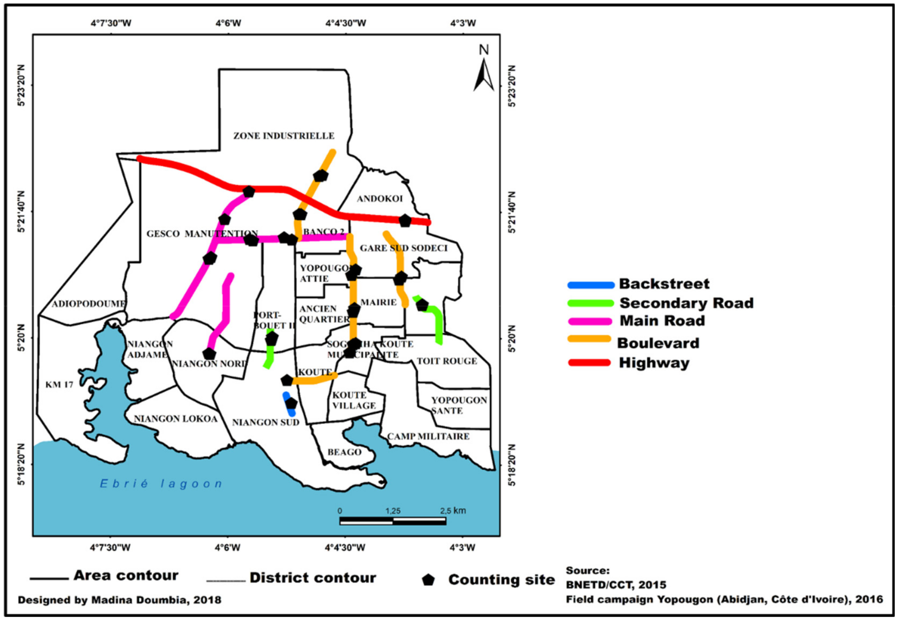
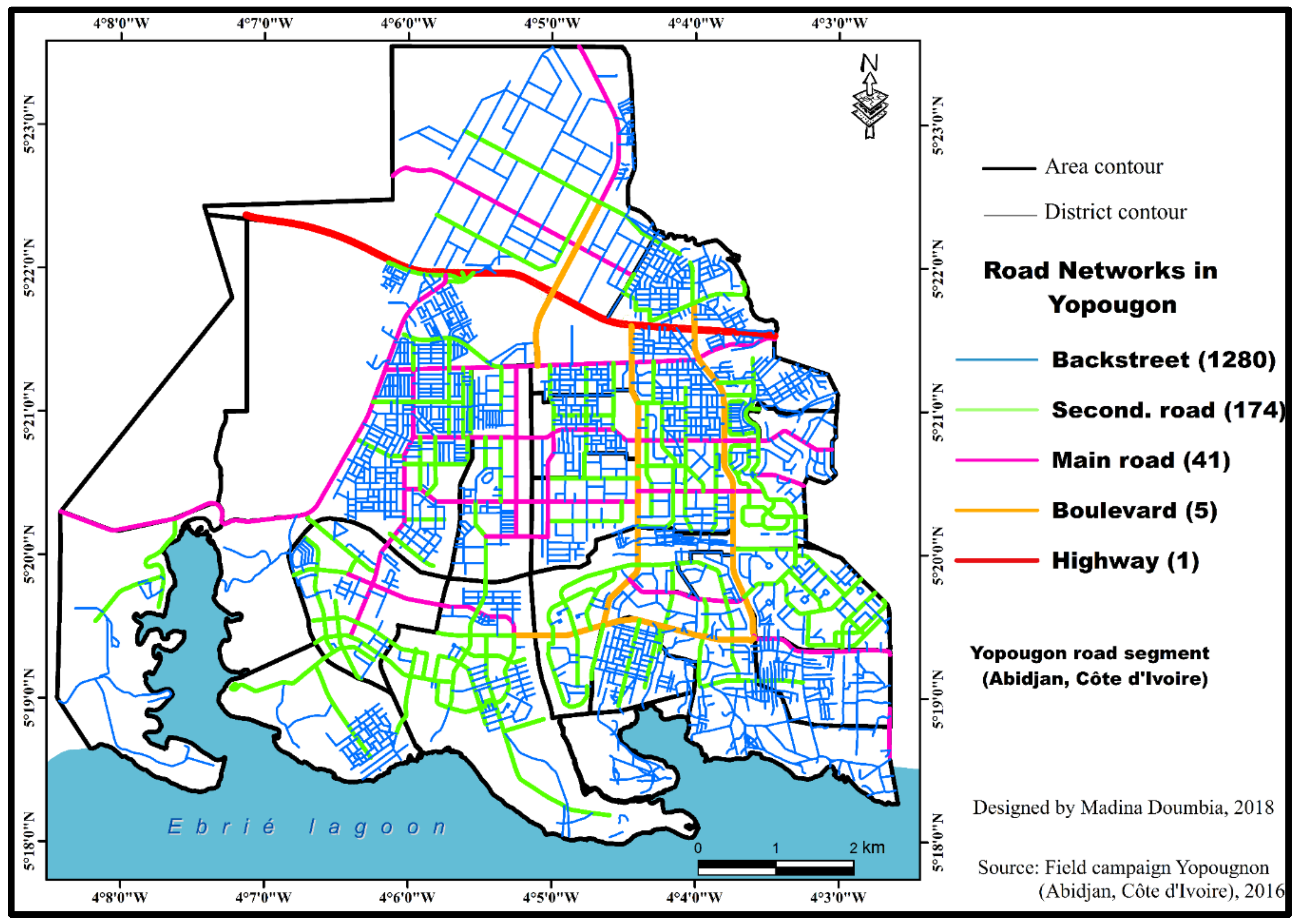
2.2. Study Area and Data

This study focuses on Yopougon city, located in the north-western part of Abidjan, the capital city of Côte d’Ivoire. The road network of Yopougon consists of urban highways, boulevards, main roads, secondary roads and backstreets (Figure 2). The fleet composition was collected by traffic questionnaire surveys and vehicle counting. Data collection and methodology of field measurements were widely discussed in Doumbia et al. [26]. Data of traffic activity such as the quantity and the type of fuel (diesel or gasoline) and the speed of each type of vehicles on all road segments collected during the field campaign were used to calculate the present emission inventory. Estimated emissions of BC, OC, NOx, CO, SO2 and NMVOC were obtained for all road segments of Yopougon using emission factors (EF) of Keita et al. [15] and Liousse et al. [13] (Table 1). Density of the different fuel types used in this study is 855 kg/m3 and 702 kg/m3 for diesel and gasoline, respectively [59].

3. Results and Discussion

3.1. Vehicle Emission Inventory by Road Segment

Using the above-described methodology, a vehicle emission inventory has been developed for 6 pollutants, namely, black carbon (BC), organic carbon (OC), carbon monoxide (CO), nitrogen oxides (NOx), sulfur dioxide (SO2) and non-methane volatile organic component (NMVOC). Emissions of pollutants from the different sampled roads during the field campaign measurements are presented in Table 2. The high emissions are obtained on the highway (HW) and are in agreement with the high vehicle flows. This confirms the fact that people who live, work or attend school near highways are subjected to an increased incidence and severe health problems which might be related to traffic emission of air pollutants [60]. Concerning the boulevards (BOs), BO1 has the highest emission rate compared to the other six. However, the most important flow was at BO6. This high emission on BO1 could be justified by the high fuel consumption on this road due to the high frequency of heavy vehicles.
Furthermore, CO is the most emitted pollutant, due to the importance of its emission factor. In addition, BC and OC emissions calculated using the emission factors (EFs) determined by Keita et al. [15] have lower values than those calculated with [13] EF values. Note that EF values of Keita et al. [15] were measured for different types of vehicles than those considered in our study.
Then, the spatial distribution of emissions for the year 2016 of each road segment in Yopougon was analyzed for the six pollutants.
Figure 3 shows spatial distribution of BC emissions of each road segment in Yopougon. This spatial distribution allows identifying high emission zones within the study area. The red line corresponds to areas of high emissions with values between 18.1 × 10³ and 180 × 103 g/d on the highway. The blue line corresponds to inside roads, so-called “backstreets”, and is associated with weak vehicle emission varying between 2.8 and 1000 g/d. Vehicle emissions for boulevards, main roads and secondary roads are respectively shown by orange, pink and green lines.
Furthermore, the area presenting the highest BC emission rate is located around the industrial zone, the highway, the boulevards and the main road intersections. Emissions from the total number of backstreets (BSs) in Yopougon (Figure 2) are the highest compared to the total roads in the city. These high emissions in the BSs are linked to a high presence of personal cars and intracommunal taxis, and by the fact that BSs represent approximately 85% of the total road network in Yopougon. Moreover, BSs are mainly used to access residential areas. Consequently, they are often crowded by vehicles with very low speeds due to the presence of speed-humps, potholes, narrow streets and poor road maintenance leading to more travelling time inducing higher fuel consumption and consequently, higher emissions.

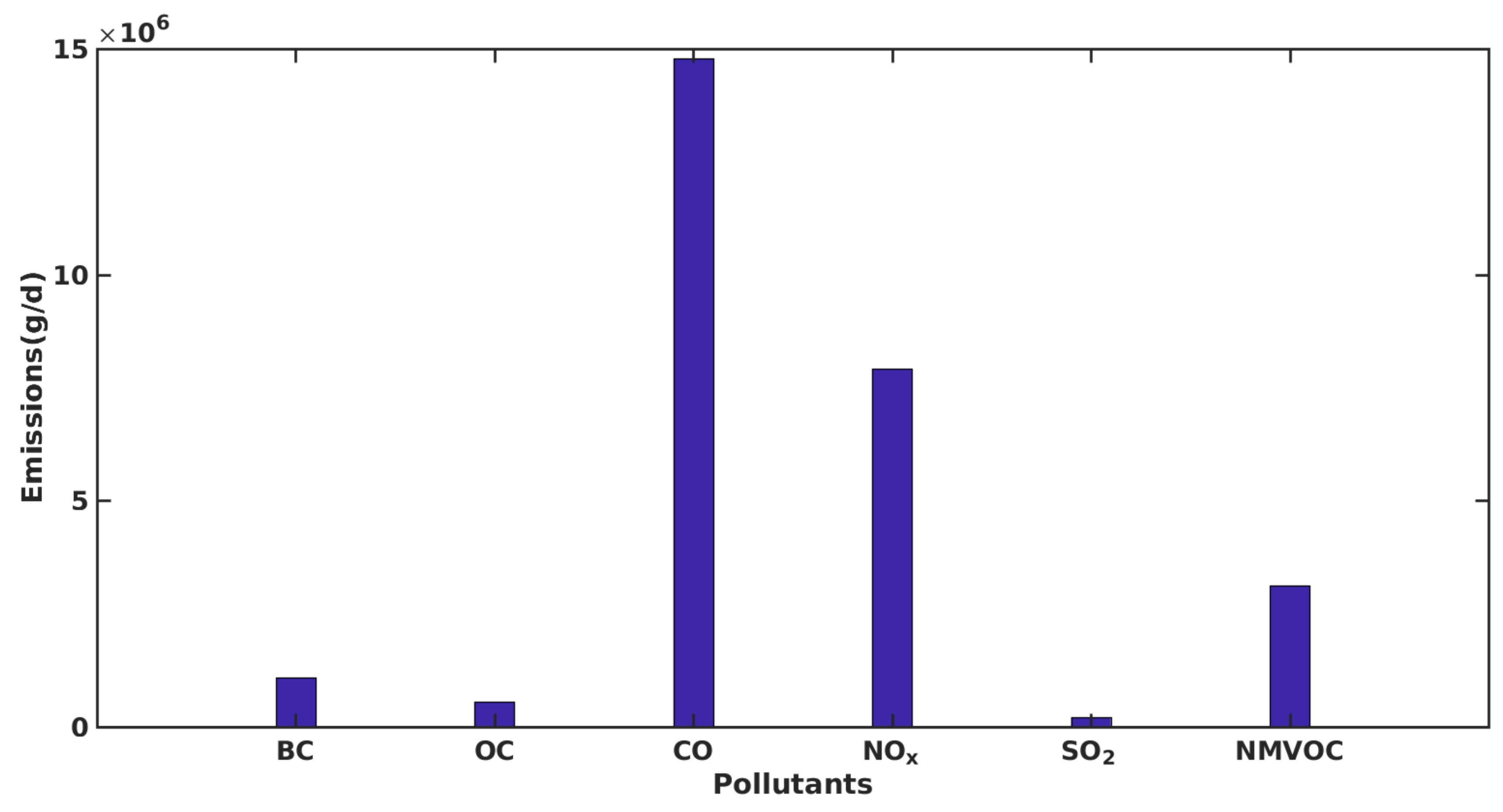
3.2. Road Traffic Emission Inventory in Yopougon

Figure 4 presents daily traffic emission inventories for BC, OC, CO, NOx, SO2 and NMVOC pollutants in Yopougon. The total traffic emission is defined as the sum of different vehicle emissions in each road segment. The two highest emitted gases are CO (14.8 t/d) and NOx (7.9 t/d). The predominance of CO and NOx is coherent since they are considered as major traffic pollution tracers [61,62,63].
CO is known to be produced by incomplete combustion. In terms of traffic emissions, CO can be found close to areas such as garages where engines are switched on or in open areas such as parking areas due to additional emission caused by ignition start [64,65,66]. Sudden stopping as well as traffic jams may contribute to an increase in CO emission concentration. Furthermore, abundance of old vehicles in Yopougon may lead to incomplete combustion contributing to increased CO emissions. In previous studies, high CO concentrations found in Ibadan (Nigeria) have been associated with high traffic rate in traffic congestion conditions observed during morning and evening traffic peaks [67]. In addition, as shown in Table 1, high CO emissions during high traffic flow is associated with high diesel (37 g/kg) and gasoline (300 g/kg) emission factors. These results are in agreement with previous works in urban areas which underlined that CO was the major pollutant in the traffic sector and greatly contributes to vehicle emission levels due to high traffic count [63,64,68].
High NOx emissions may also be explained by the presence of traffic congestion and old vehicles with no catalytic converters. This may have an impact on human health by contributing to increased respiratory and cardiovascular mortality rates [32,69,70]. Moreover, as shown in Table 1, diesel vehicles emit more NOx than gasoline vehicles due to their higher emission factor (EF). Therefore, the Yopougon fleet composed of 74% diesel vehicles, contributes to higher NOx emissions. Moreover, older ones are the diesel vehicles, and have higher NOx emission factor and emissions [68,69,70,71]. This is the case in Yopougon with more than 60% of vehicles older than 10 years [26].
Finally, NOx concentration measurement in several African cities showed an increasing trend due to poor urban traffic management, illegal roadway blockages and old diesel vehicles [26,30,72,73]. Agyemang-Bonsu et al. [74] have shown a similar trend with NOx increase from 5.4 to 7.3 Gg in Kumasi (Ghana) between 2000 and 2005.
Figure 4 also shows that total NMVOC emissions are significant although they are lower than those of CO and NOx. In addition, significant particulate emissions are represented by BC (1.09 t/d), twice as high as OC (0.56 t/d). BC is a relevant indicator of particulate pollution in road traffic. These high emissions are related to diesel engines, vehicle age and the absence of a particulate filter.
Finally, the lowest exhaust emission rates were recorded for SO2, which was 70 times lower than CO (~0.21 t/d). These low SO2 emissions were found in the concentrations measured in situ. Indeed, a recent study in Abidjan has shown that SO2 concentrations measured using passive tubes remained constant between 2015 (1.4 ± 0.7 ppb) and 2016 (1.3 ± 0.6 ppb) [75]. Although the levels of SO2 concentrations in the atmosphere are stable and not yet alarming, SO2 pollution still exists in Côte d’Ivoire. This is due to the sulfur content of the fuel produced and marketed, which is high and over 2000 ppm [76]. Therefore, we can reduce emissions with sulfur-free fuel in Côte d’Ivoire to avoid health and environmental risks. For instance, in Ibadan (Nigeria), in situ measurements show that no SO2 emissions are measured at the traffic source [67], reflecting the use of sulfur-free gasoline. The next subsection will examine various emissions by vehicle type.

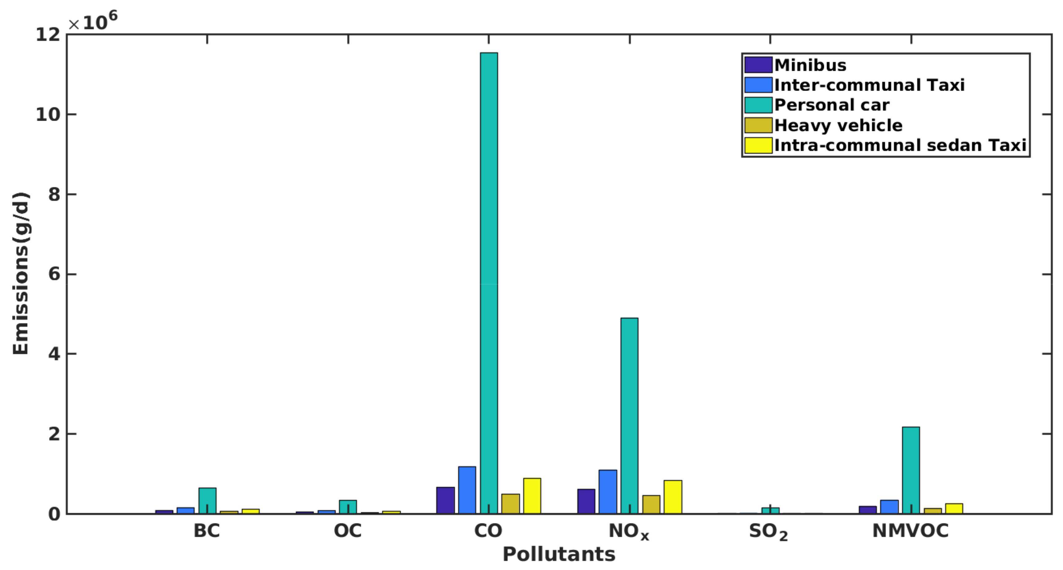
3.3. Contribution to Emissions per Vehicle Type

Traffic emissions in Yopougon result from various vehicle types. Figure 5 shows emissions for personal cars (PCs), local public taxis called intra-communal sedan taxis or “Wôrô wôrô” (WRs), inter-communal taxis (TAs), small buses or minicars known as minibuses or “Gbaka” (GBs) and heavy vehicles (buses, trucks and long vehicles) (HVs). It can be observed that PCs have a high contribution to the total emissions (e.g., 60% for BC) for each studied pollutant.
This high contribution by PCs is linked to their large number (36% of vehicles are PCs). Indeed, insecurity, poor organization and management of urban transport encourage a large majority of people to buy personal cars. Low contributions are recorded for HV (5% of vehicles are HVs), which is due to the fact that their vehicle flow or volume per day is low, although the highest fuel consumption was recorded for HVs [26]. Figure 5 also showed that WRs have a significant emission contribution after PCs. This might be related to their driving patterns: in general, WRs were observed performing several speedups, slowdowns, stops and starts, which result in increased levels of emissions [40]. Figure 5 also shows a predominance of CO emissions followed by NOx by personal cars (PCs) for all types of vehicles. In addition, PCs are the only vehicle types that use gasoline as a fuel (26% of personal car use gasoline as highlighted in Doumbia et al. [26]), thus contributing to high CO emissions. Indeed, as previously mentioned, gasoline vehicles emit more than 80 times the CO emitted by diesel engines (Table 1). The observed CO peak was also recorded by previous works [72,73,77]. Gasoline combustion is known to produce more emission due to evaporation process occurring in the engine. Furthermore, PC with air conditioner systems may induce more fuel consumption, explaining the significant CO emissions [72,78].
Figure 5 also shows that BC emissions in Yopougon are twice as high as OC emissions ranging between 1.15 and 0.59 t/d (PCs), 0.13 and 0.06 t/d (WRs), 0.16 and 0.08 t/d (TAs), 0.09 and 0.04 t/d (GBs) and 0.06 and 0.03 t/d (HVs). This was also observed in Katmandu (India) in 2010 with 2.16 Gg and 0.78 Gg, respectively, measured for BC and OC [79]. It is due to the predominance of diesel vehicles, with more significant EF values for BC than for OC. Indeed, in Doumbia et al. [26] we may observe the high rate of diesel vehicles (74% of personal cars and 100% of other type of vehicles). This pattern is also in agreement with studies by Franco et al. [80] and Sindhwani and Goyal [63] who highlighted that diesel vehicles are found to be the major contributors, respectively, of BC emissions in Bogota (Colombia), and BC and OC emissions in Delhi (India). It is interesting to recall that the opposite situation of BC and OC relative abundance is observed in anthropogenic emissions for sources such as domestic fires, industries, biomass burning and thermal central [8,81,82,83,84]. Moreover, in our study, motorcycles were not considered, because in the Yopougon (Abidjan, Côte d’Ivoire) area, these types of vehicles are rare (3% in 1998) contrarily to other West African cities such as Ouagadougou in Burkina Faso (58% in 2006), Cotonou in Benin (46% in 2001), Lomé in Togo (60% in 2000) and Bamako in Mali (56% in 2006), where the most common mode of transport is the motorcycle taxi [85,86,87,88,89]. It is important noting that in West Africa, higher emissions factors of OC than of BC have been measured by Keita et al. [15] for two wheeled vehicles, whereas in Hanoi (Vietnam) and Bangkok (Thailand), it was found that motorcycles induced more BC and CO emissions than other vehicles [79].

3.4. Contribution to Emissions per Vehicle and Road Type

Table 3 displays the emission rates of the different pollutants per road class in Yopougon: highway (HW), boulevard (BO), main road (MR), secondary road (SR) and backstreet (BS). It shows that for each pollutant, a lower emission rate is produced by WR on the HW. The highest contribution to BC emissions of vehicles on the highway is from personal cars (70.2%), which is followed in decreasing order by TAs (13.1%), HVs (9.8%), GBs (6.4%) and WRs (0.4%). While for BC on the main road, the PC (45.6%) is followed in decreasing order by the WR (20.74%), the TA (15.21%), the GB (11.65%) and the HW (6.79%). The same trend is observed for OC emissions. The emission rate of HVs is higher than that of GBs and WRs on HWs for all pollutants. It emphasizes the involvement of HVs in emissions on the HW compared to these two types of vehicles. However, HVs contribute little to total emissions although fuel consumption by this type of vehicle is the highest. This low contribution by HVs to total emissions could be related to their low level of use on all other road classes [26]. In fact, HVs are used as a means of transport for goods and building materials (sand) and people (passengers, workers and schoolchildren) inside and outside the district. They travel at specific times according to their tasks. In addition, the HW serves as a gateway to and from the industrial zone for the HVs. As for the high pollutant emissions due to the WRs on the MRs and SRs, they can be explained by the high traffic volume on these roads [26]. In fact, WRs use the highway (HW) at specific times to overcome traffic jams on other roads in the district. In addition, passenger cars are present at all times on all the roads in the district of Yopougon.

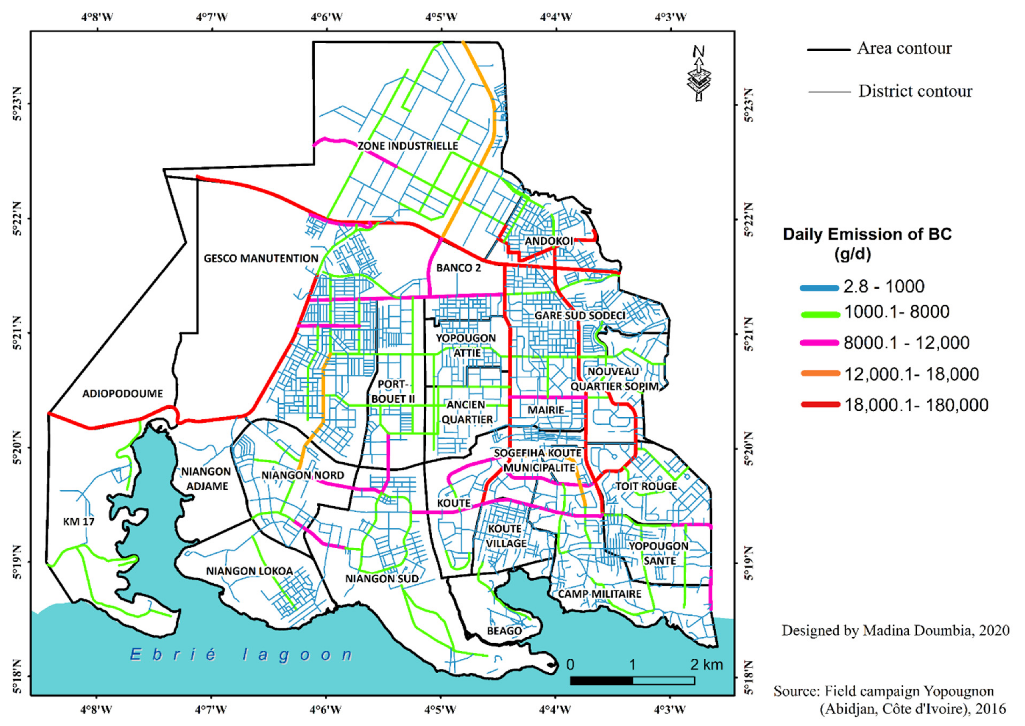
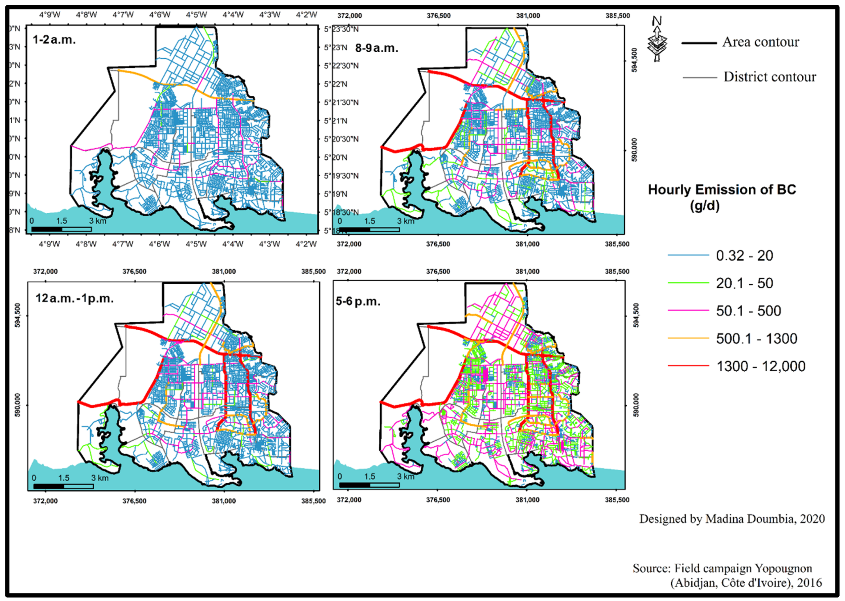
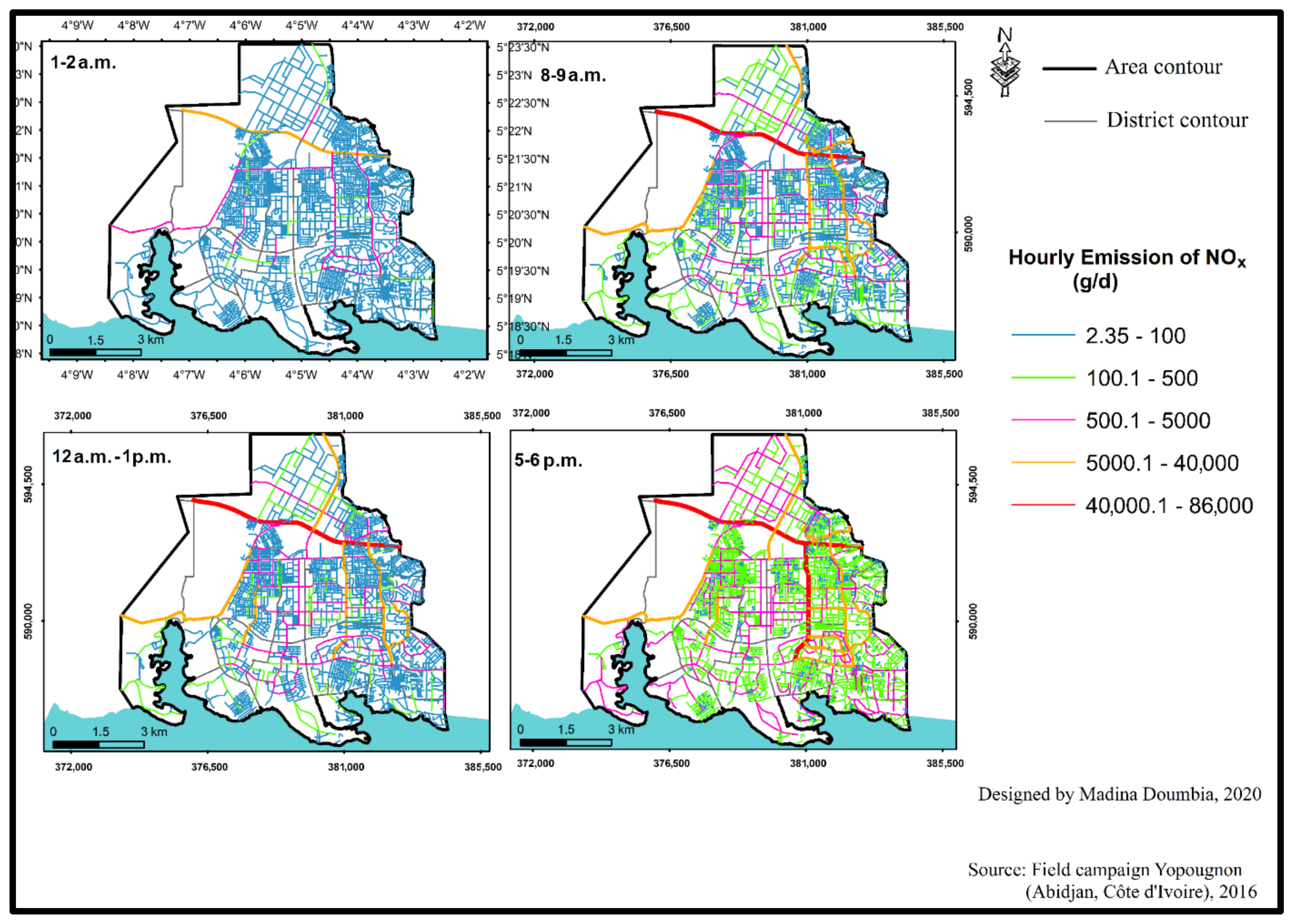
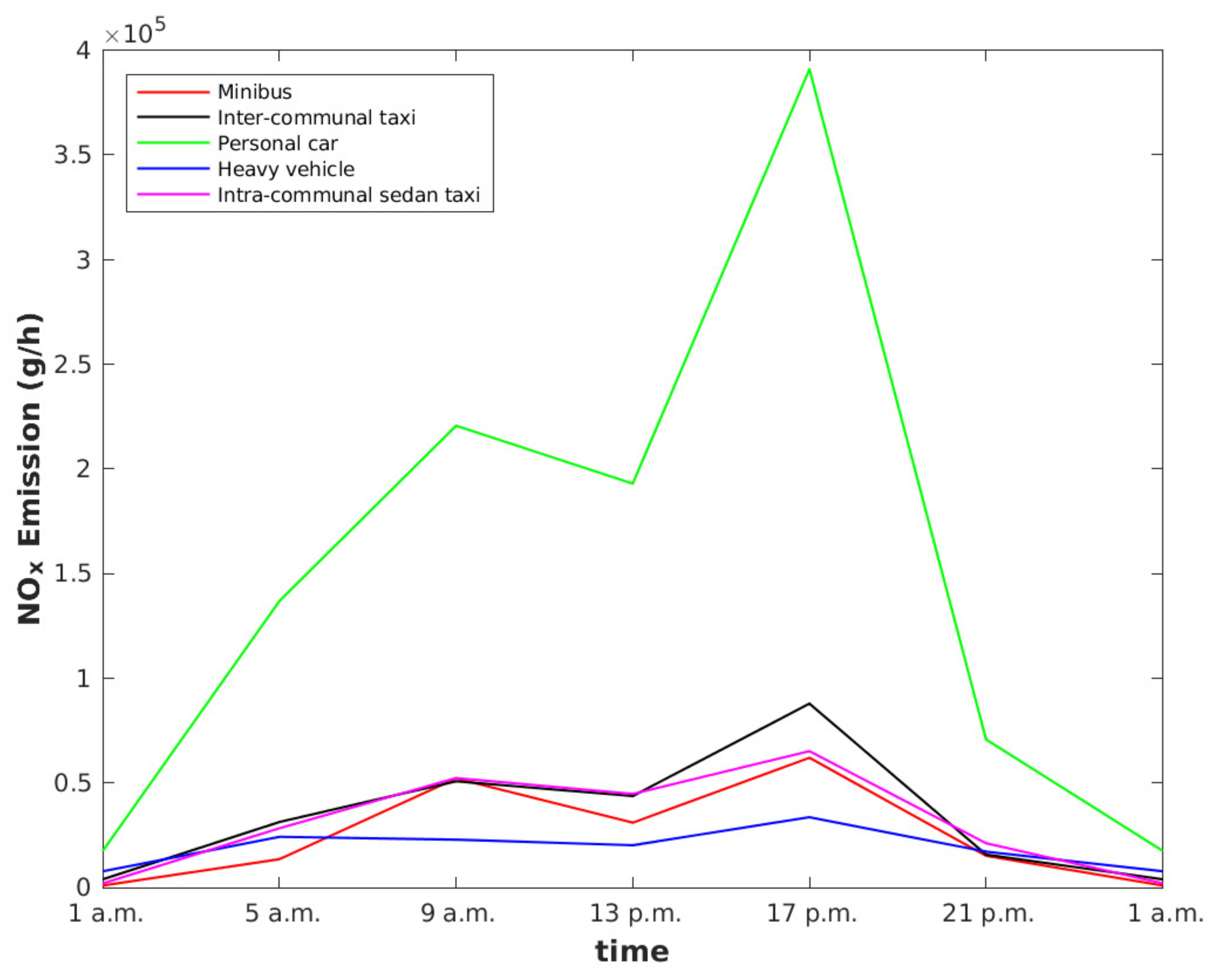
3.5. Spatial and Temporal Variation of Vehicle Emissions

Emission per hour is calculated for a better characterization of the spatial distribution of emissions in Yopougon. Figure 6 and Figure 7 display the spatial distribution of BC and NOx emissions at different times of the day (1–2 a.m., 8–9 a.m., 12 a.m.–1 p.m. and 5–6 p.m.). Red lines correspond to areas of high emissions with values between 1300 and 12,000 g/d for BC and 40,000 and 86,000 g/d for NOx. Blue lines correspond to areas of low emissions (0.32 to 20 g/d for BC and 2.35 to 100 g/d for NOx). This spatial distribution of emissions displayed through these maps allows for the identification of the different areas with high emissions associated with intense traffic activities. In addition, high emissions in the urban area of Yopougon are also observed during the off-peak hours such as 1 to 2 a.m. (at night) on the highway axis in orange. Significant emissions are also observed at peak hours such as 5 to 6 p.m. (in the evening) due to the high rate of traffic at these times.
Figure 8 illustrates the diurnal cycle of emission of NOx and shows that daily traffic emission of NOx varies throughout the day with a high contribution from personal cars. Two emission peaks are found in the morning (9 a.m.) and in the afternoon (5 p.m.) while a decrease in emissions is observed at 1 p.m. for the different types of vehicles. These two peaks of emission are associated with vehicle flux peaks, occurring in time periods when most people go to work (morning peak) and go home again (evening peak) inducing high traffic volume [26,90]. This study of the diurnal cycle of emissions is very important because it allows examination of the pollution at each time, thus to set up strategies to reduce the associated health risks. Emissions of NOx estimated at the level of individual road segments and varying by time of day in the city of Montreal (Canada) are used as input data of models [91].

3.6. Comparison with Other Emission Inventories

Table 4 presents the comparison of emissions from this work (Yopougon in 2016) with those from inventories of Liousse et al. [13] and Keita et al. [14]. These two inventories are on a regional scale, whereas in this study emission inventories are on a local scale. It is therefore appropriate to bring the regional studies to the local scale to obtain emissions in the study area (Yopougon). A “downscaling” method was performed for this purpose. The latter consists of extracting information from a larger scale to adapt to a smaller scale. For comparison, EFs of Liousse et al. [13] and new EFs of Keita et al. [15], measured as part of the Dynamics-Aerosol-Chemistry-Cloud Interactions in West Africa (DACCIWA) program and specific to our study area were used to estimate emissions (Table 4). Results show that BC emission values given by this study using the EFs of Keita et al. [15] and Liousse et al. [13] are 6–9 times higher than BC emissions of Liousse et al. [13], respectively. BC emissions of Keita et al. [14] (0.29 t/d) established for the year 2015 using EFs of Keita et al. [15], are twice as low as those of this study (0.71 t/d). These differences may be explained, on the one hand, by the uncertainty related to the fuel consumption data from the regional and national databases used in these two inventories; fuel consumption data which are crucial parameters in traffic emission estimation in the West African region [13,91]. Furthermore, it should be recalled that this inventory is based on local data of fuel consumption collected during field measurements. On the other hand, Keita et al. [15] showed that the EF values measured for gasoline are higher than those used in Liousse et al. [13] (4 times higher for BC and twice as high for OC), while they are slightly lower for diesel. This means that the use of Liousse et al. [13] EFs underestimates BC and OC emissions for on-road gasoline engines while they are of the same order of magnitude for on-road diesel engines.
Regarding OC, Table 4 shows slightly similar traffic emissions for this study and Liousse et al. [13] both using Liousse et al. [13] as the EF (0.56 t/d and 0.50 t/d, respectively). However, a difference exists when comparing OC emissions between this study and Keita et al. [14], using both EFs of [15]. Indeed, Keita et al.’s [14] values are about twice as high as those of our study (0.93 t/d and 0.48 t/d, respectively). It can be also noted that Keita et al.’s [14] values are twice as high as those of [12].
Briefly, local BC and OC emissions from traffic sources in this study are a factor of two larger and smaller, respectively, compared to Keita et al. [14] using the same emission factors. These differences can be explained by different factors such as considerable change in anthropogenic activities, EFs and spatial resolution. Regarding changes in anthropogenic activities, for example, high urbanization rates from 2005 to 2015 may be noted which lead to the highest number of vehicles and emissions. Secondly, the EFs of Keita et al. [15] took into account the different types of vehicles as well as age. EF is strongly dependent on vehicle age. The older the vehicles, the EF values for carbonaceous particles are higher [15]. It is worth noting that the EFs of Liousse et al. [13] are higher than those of Keita et al. [15] for diesel (for BC) and gasoline (for OC) explaining the higher emissions of this study found with EFs of Liousse et al. [13] compared to Keita et al. [14]. Finally, spatial resolution may also impact emission estimates by the use of fine resolutions. Spatial resolution of Liousse et al.’s [13] inventory was 25 km whilst 12.5 km for Keita et al. [14] and local for this study. Tan et al. [42] have shown that the emission inventory is improved by using finer resolution grids.

4. Conclusions

This study investigates emissions of six pollutants of major interest for air quality and their impacts such as black carbon (BC), organic carbon (OC), carbon monoxide (CO), nitrogen oxides (NOx), sulfur dioxide (SO2) and non-methane volatile organic component (NMVOC) from traffic in urban areas in Yopougon (Abidjan, Côte d’Ivoire). This study is based on a bottom-up methodology using local data of fuel consumption, as well as the use of the EFs of Liousse et al. [13] and the new realistic EFs for particulate matter (BC and OC) of Keita et al. [15] obtained during the DACCIWA campaign.
It was observed that the personal car (PC) vehicle type yielded the highest contribution to total emission in terms of proportion due to their number in Yopougon. Contribution to BC and OC emissions on the highway is significant for personal cars (PCs) followed by inter-communal taxis (TAs), heavy vehicles (HVs), minibuses (“Gbaka” or GBs) and intra-communal taxis (“Wôrô wôrô” or WRs). On the main roads, important contributions are observed for PCs, followed by WRs, for TAs, for GBs and for HVs. This is a first attempt to calculate emissions at a local scale including a comparison with regional estimates (interpolated emissions for Yopougon from downscaling approach, distributed with the population density). In addition, local emissions of BC and OC from traffic sources in this study are a factor of two larger and smaller, respectively, than the regional emissions using the same emission factors. Differences between these two emissions are due to fuel consumption data. For this study, we considered local data of fuel consumption per vehicle and fuel types, obtained from a field investigation—a local approximation. While regional emissions inventories are estimated using the International Energy Agency (IEA) fuel consumption database, available at broader country scale and fuel type.
As a perspective, the inventory resulting from our study is a significant novel contribution to the body of science since it will allow modeling of air quality and health in Yopougon. This work focused on the traffic in a locality of Abidjan where other sources of anthropogenic emissions may be observed. Thus, it needs to be completed through the integration of the other sources such as industrial, residential, landfill and charcoal making emissions.

Author Contributions

Methodology, M.D., S.K., E.-M.A., C.L. and S.S.; organization and writing paper, M.D., A.A.K., S.S., N.E.T., A.D. (Arona Diedhiou), and V.Y.; software, M.D., A.D. (Alima Dajuma), M.Z. and K.K.; validation, M.D., A.A.K., C.L. and V.Y.; investigation, M.D., M.Z., A.D. (Alima Dajuma) and A.B.; reading and following work, M.D., A.A.K., S.S., N.E.T., C.L., A.D. (Arona Diedhiou) and V.Y. All authors have read and agreed to the published version of the manuscript.

Funding

This work was supported by the Centre d’Excellence Africain sur le Changement Climatique, la Biodiversité et l’Agriculture Durable, Non-WASCAL-Sponsored West African Nationals, by Programme d’Appui Stratégique à la Recherche Scientifique (PASRES). It is also a contribution to the project PASMU (Atmospheric Pollution in Urban Areas and Impact on Health) funded by the Education and Research Ministry of Côte d’Ivoire, in the frame of the Debt Reduction-Development Contracts (C2Ds) managed by the Institute of Research for Development (IRD, France). The authors also thank IRD and the Institute of Geosciences for Environment (IGE, University Grenoble Alpes) for providing support via grant number “UMR IGE Imputation 252RA5”.

Acknowledgments

This study is a contribution to the PASMU project.

Conflicts of Interest

We have no conflict of interest.

References

  1. Konare, A.; Zakey, A.S.; Solmon, F.; Giorgi, F.; Rauscher, S.; Ibrah, S.; Bi, X. A regional climate modeling study of the effect of desert dust on the west african monsoon. J. Geophys. Res. Atmos. 2008, 113. [Google Scholar] [CrossRef]
  2. Solmon, F.; Mallet, M.; Elguindi, N.; Giorgi, F.; Zakey, A.; Konaré, A. Dust aerosol impact on regional precipitation over western Africa, mechanisms and sensitivity to absorption properties. Geophys. Res. Lett. 2008, 35. [Google Scholar] [CrossRef]
  3. Touré, N.; Konaré, A.; Silué, S. Intercontinental transport and climatic impact of saharan and sahelian dust. Adv. Meteorol. 2012, 2012. [Google Scholar] [CrossRef]
  4. Silue, S.; Konare, A.; Diedhiou, A.; Yoboue, V.; Toure, D.E.; Assamoi, P. Spatial and temporal variability of windborne dust in the Sahel-Sahara zone in relation with synoptic environment. Sci. Res. Essays 2013, 8, 705–717. [Google Scholar]
  5. Van der Werf, G.R.; Randerson, J.T.; Giglio, L.; Collatz, G.J.; Mu, M.; Kasibhatla, P.S.; Morton, D.C.; DeFries, R.S.; Jin, Y.V.; van Leeuwen, T.T. Global fire emissions and the contribution of deforestation, savanna, forest, agricultural and peat fires (1997–2009). Atmos. Chem. Phys. 2010, 10, 11707–11735. [Google Scholar] [CrossRef] [Green Version]
  6. Van der Werf, G.R.; Peters, W.; Van Leeuwen, T.T.; Giglio, L. What could have caused pre-industrial biomass burning emissions to exceed current rates? Clim. Past 2013, 9, 289–306. [Google Scholar] [CrossRef] [Green Version]
  7. Andela, N.; van der Werf, G.R. Recent trends in African fires driven by cropland expansion and El Niño to La Niña transition. Nat. Clim. Chang. 2014, 4, 791–795. [Google Scholar] [CrossRef]
  8. Liousse, C.; Galy-Lacaux, C.; Ndiaye, S.A.; Diop, B.; Ouafo, M.; Assamoi, E.M.; Gardrat, E.; Castera, P.; Rosset, R.; Akpo, A.; et al. Real time black carbon measurements in west and central Africa urban sites. Atmos. Environ. 2012, 54, 529–537. [Google Scholar]
  9. Wiedinmyer, C.; Akagi, S.K.; Yokelson, R.J.; Emmons, L.K.; Al-Saadi, J.A.; Orlando, J.J.; Soja, A.J. The fire INventory from NCAR (FINN): A high resolution global model to estimate the emissions from open burning. Geosci. Model. Dev. 2011, 4, 625. [Google Scholar] [CrossRef] [Green Version]
  10. N’Datchoh, E.T.; Diallo, I.; Konare, A.; Silue, S.; Ogunjobi, K.O.; Diedhiou, A.; Doumbia, M. Dust induced changes on the west African summer monsoon features. Int. J. Climatol. 2017, 38, 452–466. [Google Scholar] [CrossRef] [Green Version]
  11. Ichoku, C.; Ellison, L.T.; Willmot, K.E.; Matsui, T.; Dezfuli, A.K.; Gatebe, C.K.; Wang, J.; Wilcox, E.M.; Lee, J.; Adegoke, J.; et al. Biomass burning, land-cover change and the hydrological cycle in northern sub-Saharan Africa. Environ. Res. Lett. 2016, 11, 095005. [Google Scholar] [CrossRef] [Green Version]
  12. Assamoi, E.-M.; Liousse, C. A new inventory for two-wheel vehicle emissions in west Africa for 2002. Atmos. Environ. 2010, 44, 3985–3996. [Google Scholar] [CrossRef]
  13. Liousse, C.; Assamoi, E.; Criqui, P.; Granier, C.; Rosset, R. Explosive growth in African combustion emissions from 2005 to 2030. Environ. Res. Lett. 2014, 9, 035003. [Google Scholar] [CrossRef]
  14. Keita, S.; Liousse, C.; Assamoi, E.-M.; Doumbia, T.; Touré, N.; Gnamien, S.; Elguindi, N.; Granier, C.; Yoboué, V. African anthropogenic emissions inventory for gases and particles from 1990 to 2015. Earth Syst. Sci. Data Discuss. 2020, 1–29. [Google Scholar] [CrossRef]
  15. Keita, S.; Liousse, C.; Yoboú, V.; Dominutti, P.; Guinot, B.; Assamoi, E.M.; Borbon, A.; Haslett, S.L.; Bouvier, L.; Colomb, A. Particle and VOC emission factor measurements for anthropogenic sources in west Africa. Atmos. Chem. Phys. 2018, 18, 7691–7708. [Google Scholar] [CrossRef] [Green Version]
  16. Liousse, C. Updated African biomass burning emission inventories in the framework of the AMMA-IDAF program, with an evaluation of combustion aerosols. Atmos. Chem. Phys. 2010, 10, 9631–9646. [Google Scholar] [CrossRef] [Green Version]
  17. Laborde, M.; Crippa, M.; Tritscher, T.; Jurányi, Z.; Decarlo, P.F.; Temime-Roussel, B.; Marchand, N.; Eckhardt, S.; Stohl, A.; Baltensperger, U. Black carbon physical properties and mixing state in the European megacity Paris. Atmos. Chem. Phys. 2013, 13, 5831–5856. [Google Scholar] [CrossRef] [Green Version]
  18. Freney, E.J.; Sellegri, K.; Canonaco, F.; Colomb, A.; Borbon, A.; Michoud, V.; Doussin, J.-F.; Crumeyrolle, S.; Amarouche, N.; Pichon, J.-M.; et al. Characterizing the impact of urban emissions on regional aerosol particles: Airborne measurements during the MEGAPOLI experiment. Atmos. Chem. Phys. 2014, 14, 1397–1412. [Google Scholar] [CrossRef] [Green Version]
  19. Huang, X.; Song, Y.; Zhao, C.; Cai, X.; Zhang, H.; Zhu, T. Direct radiative effect by multicomponent aerosol over China. J. Clim. 2015, 28, 3472–3495. [Google Scholar] [CrossRef]
  20. Pu, W.; Wang, X.; Zhang, X.; Ren, Y.; Shi, J.-S.; Bi, J.-R.; Zhang, B.-D. Size distribution and optical properties of particulate matter (PM10) and black carbon (BC) during dust storms and local air pollution events across a loess plateau site. Aerosol Air Qual. Res. 2015, 15, 2212–2224. [Google Scholar] [CrossRef] [Green Version]
  21. Wang, Q.; Huang, R.-J.; Cao, J.; Tie, X.; Shen, Z.; Zhao, S.; Han, Y.; Li, G.; Li, Z.; Ni, H.; et al. Contribution of regional transport to the black carbon aerosol during winter haze period in Beijing. Atmos. Environ. 2016, 132, 11–18. [Google Scholar] [CrossRef]
  22. Oguntoke, O.; Yussuf, A.S. Air pollution arising from vehicular emissions and the associated human health problems in abeokuta metropolis, Nigeria. Asset Int. J. Ser. A 2008, 8, 119–132. [Google Scholar]
  23. Ekpenyong, C.E.; Ettebong, E.O.; Akpan, E.E.; Samson, T.K.; Daniel, N.E. Urban city transportation mode and respiratory health effect of air pollution: A cross-sectional study among transit and non-transit workers in Nigeria. BMJ Open 2012, 2, e001253. [Google Scholar] [CrossRef] [Green Version]
  24. Ndoke, P.N.; Jimoh, O.D. Impact of Traffic Emission on Air Quality in a Developing City of Nigeria. Available online: http://www.journal.au.edu/au_techno/2005/apr05/vol8no4_abstract10.pdf (accessed on 30 January 2021).
  25. Naidja, L.; Ali-Khodja, H.; Khardi, S. Particulate matter from road traffic in Africa. J. Earth Sci. Geotech. Eng. 2017, 7, 289–304. [Google Scholar]
  26. Doumbia, M.; Toure, N.; Silue, S.; Yoboue, V.; Diedhiou, A.; Hauhouot, C. Emissions from the road traffic of west African cities: Assessment of vehicle fleet and fuel consumption. Energies 2018, 11, 2300. [Google Scholar] [CrossRef] [Green Version]
  27. Hopkins, J.R.; Evans, M.J.; Lee, J.D.; Lewis, A.C.; Marsham, J.H.; McQuaid, J.B.; Parker, D.J.; Stewart, D.J.; Reeves, C.E.; Purvis, R.M. Direct estimates of emissions from the megacity of Lagos. Atmos. Chem. Phys. 2009, 9, 8471–8477. [Google Scholar] [CrossRef] [Green Version]
  28. Armah, F.A.; Yawson, D.O.; Pappoe, A.A. A systems dynamics approach to explore traffic congestion and air pollution link in the city of Accra, Ghana. Sustainability 2010, 2, 252–265. [Google Scholar] [CrossRef] [Green Version]
  29. Ameh, J.A.; Tor-Anyiin, T.A.; Eneji, I.S. Assessment of some gaseous emissions in traffic areas in Makurdi metropolis, Benue State, Nigeria. Open J. Air Pollut. 2015, 4, 175. [Google Scholar] [CrossRef] [Green Version]
  30. Moselakgomo, M.; Naidoo, M.; Letebele, M.O. The indicative effects of inefficient urban traffic flow on fuel cost and exhaust air pollutant emissions. In Proceedings of the 34th Annual Southern African Transport Conference, Pretoria, South Africa, 6–9 July 2015. [Google Scholar]
  31. Gnamien, S.; Yoboué, V.; Liousse, C.; Keita, S.; Bahino, J.; Siélé, S.; Diaby, L. Particulate pollution in Korhogo and Abidjan (Cote d’Ivoire) during the dry season. Aerosol Air Qual. Res. 2020, 21, 20020. [Google Scholar] [CrossRef]
  32. Alshetty, V.D.; Kuppili, S.K.; Nagendra, S.S.; Ramadurai, G.; Sethi, V.; Kumar, R.; Sharma, N.; Namdeo, A.; Bell, M.; Goodman, P. Characteristics of tail pipe (Nitric oxide) and resuspended dust emissions from urban roads–A case study in Delhi city. J. Transp. Health 2019, 17, 100653. [Google Scholar] [CrossRef]
  33. Goodrick, S.L.; Achtemeier, G.L.; Larkin, N.K.; Liu, Y.; Strand, T.M. Modelling smoke transport from wildland fires: A review. Int. J. Wildland Fire 2013, 22, 83. [Google Scholar] [CrossRef]
  34. Paugam, R.; Wooster, M.; Freitas, S.; Val Martin, M. A review of approaches to estimate wildfire plume injection height within large-scale atmospheric chemical transport models. Atmos. Chem. Phys. 2016, 16, 907–925. [Google Scholar] [CrossRef] [Green Version]
  35. Requia, W.J.; Higgins, C.D.; Adams, M.D.; Mohamed, M.; Koutrakis, P. The health impacts of weekday traffic: A health risk assessment of PM2. 5 emissions during congested periods. Environ. Int. 2018, 111, 164–176. [Google Scholar] [CrossRef] [PubMed]
  36. San José, R.; Pérez, J.L.; Pérez, L.; González, R.M.; Pecci, J.; Palacios, M. Forest fire forecasting tool for air quality modelling systems. Fís. Tierra 2015, 27, 69. [Google Scholar]
  37. Shekarrizfard, M.; Valois, M.-F.; Weichenthal, S.; Goldberg, M.S.; Fallah-Shorshani, M.; Cavellin, L.D.; Crouse, D.; Parent, M.-E.; Hatzopoulou, M. Investigating the effects of multiple exposure measures to traffic-related air pollution on the risk of breast and prostate cancer. J. Transp. Health 2018, 11, 34–46. [Google Scholar] [CrossRef]
  38. Zhang, K.; Batterman, S.; Dion, F. Vehicle emissions in congestion: Comparison of work zone, rush hour and free-flow conditions. Atmos. Environ. 2011, 45, 1929–1939. [Google Scholar] [CrossRef]
  39. Zhang, X.; Craft, E.; Zhang, K. Characterizing spatial variability of air pollution from vehicle traffic around the Houston ship channel area. Atmos. Environ. 2017, 161, 167–175. [Google Scholar] [CrossRef]
  40. Zhang, K.; Batterman, S. Air pollution and health risks due to vehicle traffic. Sci. Total Environ. 2013, 450, 307–316. [Google Scholar] [CrossRef] [Green Version]
  41. Huo, H.; Zhang, Q.; He, K.; Yao, Z.; Wang, X.; Zheng, B.; Streets, D.G.; Wang, Q.; Ding, Y. Modeling vehicle emissions in different types of Chinese cities: Importance of vehicle fleet and local features. Environ. Pollut. 2011, 159, 2954–2960. [Google Scholar] [CrossRef]
  42. Tan, J.; Zhang, Y.; Ma, W.; Yu, Q.; Wang, J.; Chen, L. Impact of spatial resolution on air quality simulation: A case study in a highly industrialized area in Shanghai, China. Atmos. Pollut. Res. 2015, 6, 322–333. [Google Scholar] [CrossRef] [Green Version]
  43. Allende, D.; Ruggeri, M.F.; Lana, B.; Garro, K.; Altamirano, J.; Puliafito, E. Inventory of primary emissions of selected persistent organic pollutants to the atmosphere in the area of Great Mendoza. Emerg. Contam. 2016, 2, 14–25. [Google Scholar] [CrossRef] [Green Version]
  44. Jing, B.; Wu, L.; Mao, H.; Gong, S.; He, J.; Zou, C.; Song, G.; Li, X.; Wu, Z. Development of a vehicle emission inventory with high temporal–spatial resolution based on NRT traffic data and its impact on air pollution in Beijing–Part 1: Development and evaluation of vehicle emission inventory. Atmos. Chem. Phys. 2016, 16, 3161–3170. [Google Scholar] [CrossRef] [Green Version]
  45. Zhou, Y.; Zhao, Y.; Mao, P.; Zhang, Q.; Zhang, J.; Qiu, L.; Yang, Y. Development of a high-resolution emission inventory and its evaluation and application through air quality modeling for Jiangsu province, China. Atmos. Chem. Phys. 2017, 17, 211–233. [Google Scholar] [CrossRef] [Green Version]
  46. Ponche, J.-L.; Vinuesa, J.-F. Emission scenarios for air quality management and applications at local and regional scales including the effects of the future European emission regulation (2015) for the upper Rhine Valley. Atmos. Chem. Phys. 2005, 5, 999–1014. [Google Scholar] [CrossRef] [Green Version]
  47. Abulude, F.O.; Bahloul, M.; Adeoya, E.A.; Olubayode, S.A. A review on top-down and bottom-up approaches for air pollution studies. Preprints 2017. [Google Scholar] [CrossRef] [Green Version]
  48. Wang, H.; Chen, C.; Huang, C.; Fu, L. On-road vehicle emission inventory and its uncertainty analysis for Shanghai, China. Sci. Total Environ. 2008, 398, 60–67. [Google Scholar] [CrossRef]
  49. Wang, H.; Fu, L.; Lin, X.; Zhou, Y.; Chen, J. A bottom-up methodology to estimate vehicle emissions for the Beijing urban area. Sci. Total Environ. 2009, 407, 1947–1953. [Google Scholar] [CrossRef]
  50. Zavala, M.; Herndon, S.C.; Wood, E.C.; Jayne, J.T.; Nelson, D.D.; Trimborn, A.M.; Dunlea, E.; Knighton, W.B.; Mendoza, A.; Allen, D.T.; et al. Comparison of emissions from on-road sources using a mobile laboratory under various driving and operational sampling modes. Atmos. Chem. Phys. 2009, 9, 1–14. [Google Scholar] [CrossRef] [Green Version]
  51. Mohan, M. Performance evaluation of AERMOD and ADMS-urban for total suspended particulate matter concentrations in megacity Delhi. Aerosol Air Qual. Res. 2011. [Google Scholar] [CrossRef] [Green Version]
  52. Timmermans, R.M.A.; Denier van der Gon, H.A.C.; Kuenen, J.J.P.; Segers, A.J.; Honoré, C.; Perrussel, O.; Builtjes, P.J.H.; Schaap, M. Quantification of the urban air pollution increment and its dependency on the use of down-scaled and bottom-up city emission inventories. Urban Clim. 2013, 6, 44–62. [Google Scholar] [CrossRef]
  53. Borge García, R.; de la Paz, D.; Lumbreras, J.; Pérez, J.; Vedrenne, M. Analysis of contributions to NO2 ambient air quality levels in Madrid city (Spain) through modeling. Implications for the development of policies and air quality monitoring. J. Geosci. Environ. Prot. 2014, 2, 6–11. [Google Scholar]
  54. Pallavidino, L.; Prandi, R.; Bertello, A.; Bracco, E.; Pavone, F. Compilation of a road transport emission inventory for the province of Turin: Advantages and key factors of a bottom–up approach. Atmos. Pollut. Res. 2014, 5, 648–655. [Google Scholar] [CrossRef] [Green Version]
  55. He, J.; Wu, L.; Mao, H.; Liu, H.; Jing, B.; Yu, Y.; Ren, P.; Feng, C.; Liu, X. Development of a vehicle emission inventory with high temporal–spatial resolution based on NRT traffic data and its impact on air pollution in Beijing–Part 2: Impact of vehicle emission on urban air quality. Atmos. Chem. Phys. 2016, 16, 3171–3184. [Google Scholar] [CrossRef] [Green Version]
  56. Cooke, W.F.; Liousse, C.; Cachier, H.; Feichter, J. Construction of a 1 × 1 fossil fuel emission data set for carbonaceous aerosol and implementation and radiative impact in the ECHAM4 model. J. Geophys. Res. Atmos. 1999, 104, 22137–22162. [Google Scholar] [CrossRef]
  57. Junker, C.; Liousse, C. A global emission inventory of carbonaceous aerosol from historic records of fossil fuel and biofuel consumption for the period 1860–1997. Atmos. Chem. Phys. 2008, 1–13. [Google Scholar]
  58. Friedrich, R.; Reis, S. Emissions of Air Pollutants: Measurements, Calculations and Uncertainties; Springer Science & Business Media: Berlin, Germany, 2013. [Google Scholar]
  59. Assamoi, A.Y.E.-M. Emissions Anthropiques d’Aérosols Carbonés en Afrique en 2005 et en 2030: Élaboration e’Inventaires et Évaluation. Ph.D. Thesis, Université Paul Sabatier-Toulouse III, Toulouse, France, 2011. [Google Scholar]
  60. Barros, N.; Fontes, T.; Silva, M.P.; Manso, M.C. How wide should be the adjacent area to an urban motorway to prevent potential health impacts from traffic emissions? Transp. Res. Part A: Policy Pract. 2013, 50, 113–128. [Google Scholar] [CrossRef]
  61. Ouarzazi, J.; Terhzaz, M.; Abdellaoui, A.; Bouhafid, A.; Nollet, V.; Dechaux, J.-C. Etude descriptive de La mesure de polluants atmospheriques dans l’agglomération de Marrakech. Pollut. Atmos. 2003, 2268–3798, 137–151. [Google Scholar] [CrossRef] [Green Version]
  62. Kansal, A.; Khare, M.; Sharma, C.S. Air quality modelling study to analyse the impact of the world bank emission guidelines for thermal power plants in Delhi. Atmos. Pollut. Res. 2011, 2, 99–105. [Google Scholar] [CrossRef] [Green Version]
  63. Sindhwani, R.; Goyal, P. Assessment of traffic-generated gaseous and particulate matter emissions and trends over Delhi (2000–2010). Atmos. Pollut. Res. 2014, 5, 438–446. [Google Scholar] [CrossRef] [Green Version]
  64. Höglund, P.G. Parking, energy consumption and air pollution. Sci. Total Environ. 2004, 334, 39–45. [Google Scholar] [CrossRef]
  65. Chinrungrueng, J.; Sunantachaikul, U.; Triamlumlerd, S. Smart parking: An application of optical wireless sensor network. In Proceedings of the 2007 International Symposium on Applications and the Internet Workshops, Hiroshima, Japan, 15–19 January 2007; p. 66. [Google Scholar]
  66. Coric, V.; Gruteser, M. Crowdsensing maps of on-street parking spaces. In Proceedings of the 2013 IEEE International Conference on Distributed Computing in Sensor Systems, Cambridge, MA, USA, 20–23 May 2013; pp. 115–122. [Google Scholar]
  67. Effiong, U.E. Air pollution emission inventory along a major traffic route within Ibadan metropolis, southwestern Nigeria. Afr. J. Environ. Sci. Technol. 2016, 10, 432–438. [Google Scholar] [CrossRef] [Green Version]
  68. Semakula, M.; Inambao, F. Biodiesel, Combustion, Performance and Emissions Characteristics; Springer Nature: London, UK, 2020. [Google Scholar]
  69. Chen, Y.; Borken-Kleefeld, J. NO x emissions from Diesel passenger cars worsen with age. Environ. Sci. Technol. 2016, 50, 3327–3332. [Google Scholar] [CrossRef] [PubMed] [Green Version]
  70. Chen, Y.; Sun, R.; Borken-Kleefeld, J. On-Road NO x and smoke emissions of Diesel light commercial vehicles–combining remote sensing measurements from across Europe. Environ. Sci. Technol. 2020, 54, 11744–11752. [Google Scholar] [CrossRef] [PubMed]
  71. Smith, T.R.; Kersey, V.; Bidwell, T. The effect of engine age, engine oil age and drain interval on vehicle tailpipe emissions and fuel efficiency. Sae Trans. 2001, 1838–1861. [Google Scholar]
  72. ATMOPACA. Les Emissions Dues aux Transports Routiers Note de Synthese Realisee dans le Cadre d’un Projet Soutenu par la Region PACA et la CPA. Available online: https://www.atmosud.org/sites/paca/files/atoms/files/081105_atmopaca_note_synthese_transport_colloque_ort.pdf (accessed on 30 January 2021).
  73. Pérez-Martínez, P.J.; Fátima Andrade, M.; Miranda, R.M. Traffic-related air quality trends in São Paulo, Brazil. J. Geophys. Res. Atmos. 2015, 120, 6290–6304. [Google Scholar] [CrossRef] [Green Version]
  74. Agyemang-Bonsu, K.W.; Dontwi, I.K.; Tutu-Benefoh, D.A.; Bentil, D.E.; Boateng, O.G.; Asuobonteng, K.; Agyemang, W. Traffic-data driven modelling of vehicular emissions using COPERT III in Ghana: A case study of Kumasi. Am. J. Sci. Ind. Res. 2010, 1, 32–40. [Google Scholar]
  75. Bahino, J.; Yoboué, V.; Galy-Lacaux, C.; Adon, M.; Akpo, A.; Keita, S.; Liousse, C.; Gardrat, E.; Chiron, C.; Ossohou, M. A pilot study of gaseous pollutants’ measurement (NO 2, SO 2, NH 3, HNO 3 and O 3) in Abidjan, Côte d’Ivoire: Contribution to an overview of gaseous pollution in African cities. Atmos. Chem. Phys. 2018, 18, 5173–5198. [Google Scholar] [CrossRef] [Green Version]
  76. Boularab, I.; Elghazi, I.; Mouhaddach, O.; Kestemont, M.-P.; El Jaafari, S. Analyse Spatiale de la Pollution Particulaire au Niveau de la Ville de Meknès (Maroc)/[Spatial Analysis of Particulate Air Pollution in Meknes City (Morocco)]. Int. J. Innov. Appl. Stud. 2015, 13, 781. [Google Scholar]
  77. Atmo PACA. Inventaire des Émissions Année de Référence 2004. Pollution Atmosphérique et Gaz à Effet de Serre. Available online: https://www.atmosud.org/sites/paca/files/publications_import/files/090223_AirPACA_Rapport_Inventaire_PACA_2004_V2009_net.pdf (accessed on 30 January 2021).
  78. Joumard, R. Les Enjeux de La Pollution de l’Air des Transports. In Proceedings of the Transports et Pollution de l’Air, Avignon, France, 16–18 June 2003; pp. 233–240. [Google Scholar]
  79. Kim Oanh, N.T.; Huynh, H.V.; Saikawa, E. Comparative analysis of passenger traffic fleets in Asian cities: Technology, driving activities and emission. In Proceedings of the AGU Fall Meeting Abstracts, San Francisco, CA, USA, 14–18 December 2015. [Google Scholar]
  80. Franco, J.F.; Rojas, N.Y.; Sarmiento, O.L.; Behrentz, E. Urban air pollution in school-related microenvironments in Bogota, Colombia. Ing. E Investig. 2013, 33, 42–48. [Google Scholar]
  81. Guinot, B.; Cachier, H.; Sciare, J.; Tong, Y.; Xin, W.; Jianhua, Y. Beijing aerosol: Atmospheric interactions and new trends. J. Geophys. Res. Atmos. 2007, 112. [Google Scholar] [CrossRef] [Green Version]
  82. Sandradewi, J.; Prévôt, A.S.; Szidat, S.; Perron, N.; Alfarra, M.R.; Lanz, V.A.; Weingartner, E.; Baltensperger, U. Using aerosol light absorption measurements for the quantitative determination of wood burning and traffic emission contributions to particulate matter. Environ. Sci. Technol. 2008, 42, 3316–3323. [Google Scholar] [CrossRef] [PubMed]
  83. Pio, C.; Cerqueira, M.; Harrison, R.M.; Nunes, T.; Mirante, F.; Alves, C.; Oliveira, C.; de la Campa, A.S.; Artíñano, B.; Matos, M. OC/EC ratio observations in Europe: Re-thinking the approach for apportionment between primary and secondary organic carbon. Atmos. Environ. 2011, 45, 6121–6132. [Google Scholar] [CrossRef]
  84. Bond, T.C.; Doherty, S.J.; Fahey, D.W.; Forster, P.M.; Berntsen, T.; DeAngelo, B.J.; Flanner, M.G.; Ghan, S.; Kärcher, B.; Koch, D. Bounding the role of black carbon in the climate system: A scientific assessment. J. Geophys. Res. Atmos. 2013, 118, 5380–5552. [Google Scholar] [CrossRef]
  85. Duprez, F. Les Coûts Sociaux du Système de Transports Urbains d’Abidjan (Côte d’Ivoire). Available online: http://dev.codatu.org/wp-content/uploads/Les-co%C3%BBts-sociaux-du-syst%C3%A8me-de-transports-urbains-dAbidjan-Cote-dIvoire-F.DUPREZ.pdf (accessed on 30 January 2021).
  86. Guézéré, A. Deux Roues Motorisées et Étalement Urbain à Lomé, Quel Lien avec la Théorie des «trois Âges» de la Ville? Norois. Environ. Aménage. Soc. 2013, 41–62. [Google Scholar] [CrossRef]
  87. Kumar, A.; Barrett, F. Stuck in traffic: Urban transport in Africa. In AICD Background Paper. Available online: https://www.eu-africa-infrastructure-tf.net/attachments/library/aicd-background-paper-1-urban-trans-summary-en.pdf (accessed on 30 January 2021).
  88. Pochet, P.; Olvera, L.D.; Plat, D.; Adolehoume, A. L’usage Privé et Public des Motos dans les Villes d’Afrique Sub-Saharienne. In Public Transport Trends 2017; UITP: Brussels, Belgium, 2017; pp. 103–105. [Google Scholar]
  89. Olvera, L.D.; Plat, D.; Pochet, P.; Maïdadi, S. Motorbike taxis in the “Transport Crisis” of west and central African cities. EchoGéo 2012, 20, 15. [Google Scholar] [CrossRef] [Green Version]
  90. Kan, Z.; Tang, L.; Kwan, M.-P.; Zhang, X. Estimating vehicle fuel consumption and emissions using GPS big data. Int. J. Environ. Res. Public Health 2018, 15, 566. [Google Scholar] [CrossRef] [Green Version]
  91. Sider, T.; Alam, A.; Zukari, M.; Dugum, H.; Goldstein, N.; Eluru, N.; Hatzopoulou, M. Land-use and socio-economics as determinants of traffic emissions and individual exposure to air pollution. J. Transp. Geogr. 2013, 33, 230–239. [Google Scholar] [CrossRef]
Figure 1. Different road types of the road network in Yopougon. Red line represents the highway, blue line is for the backstreet, pink lines are the main roads, green and orange are the secondary roads and boulevards, respectively. Location of counting point of vehicle fleet composition over several road types in Yopougon in Doumbia et al. [26].
Energies 14 01111 g001
Figure 2. Yopougon network with different road segments. Number of road segments of each road type are in brackets.
Energies 14 01111 g002
Figure 3. Spatial distribution of pollutant emissions of BC for the year 2016 in Yopougon.
Energies 14 01111 g003
Figure 4. Total traffic emissions in Yopougon of BC, OC, CO, NOx, SO2 and NMVOC.
Energies 14 01111 g004
Figure 5. Traffic emission contribution by different vehicle types in Yopougon.
Energies 14 01111 g005
Figure 6. Spatial distribution of pollutant emissions of BC at different hours.
Energies 14 01111 g006
Figure 7. Spatial distribution of pollutant emissions of NOx at different hours.
Energies 14 01111 g007
Figure 8. Total vehicle emission of NOx for different vehicle types in Yopougon.
Energies 14 01111 g008
Table 1. Emissions factor (EF) of traffic sources for gasoline and diesel vehicle of different aerosols and gases from literature.
EF (g/kg)BCOCCONOxSO2NMVOC
Fuel
Diesel5.00 [13]
3.35 ± 2.20 (a) [15]
2.20 ± 1.05 (b) [15]
2.50 [13]
2.03 ± 1.13 (a) [15]
2.5 ± 1.43 (b)
37.00 [13]34.40 [13]0.72 [13]10.85 [13]
Gasoline0.15 [13]
0.62 ± 0.49 (a) [15]
0.73 [13]
1.1 ± 0.77(a) [15]
300.00 [13]19.50 [13]2.36 [13]34.00 [13]
(a) light duty vehicle (LDV) (b) heavy duty vehicle (HDV). black carbon (BC), organic carbon (OC), carbon monoxide (CO), nitrogen oxides (NOx), sulfur dioxide (SO2) and non-methane volatile organic component (NMVOC).
Table 2. Emissions of the different pollutants (g/d) on the different sampled axes of the city of Yopougon for road vehicles using emissions factors (EFs).
Road NetworkRoad NameEMISSIONS (g/d)
BC (a)BC (b)OC (a)OC (b)CO (a)NOX (a)SO2 (a)NMVOC (a)
BO13ème pont-Zone Indus19,786.0512,616.9110,167.438803.34267,924.66143,635.833799.8256,625.44
BO240-St Pierre7938.985345.904064.553388.52100,842.3557,221.081472.5421,970.10
MR1Ant Annaneraie-CHU7575.225102.713899.143271.15105,443.7055,169.051477.2222,002.43
HWBanco-1er Pont129,461.0684,700.965699.934879.391,853,499.61946,023.0225,648.34381,820.80
BO3Crf Zone-3ème pont14,942.339775.227703.576593.96213,481.14109,161.792956.8144,019.00
MR2Crf Zone-CHU6010.404005.383075.532579.4375,619.2543,275.781109.1416,551.22
BO4Kenya-Wakouboué7441.674992.333803.323171.6291,590.8453,455.371357.3420,263.24
MR3Lubafrique-Antenne_Maroc5569.683746.972183.941827.8074,161.5440,355.111059.7915,798.07
SR1Mossikro-Nouveau Qrt10,281.606928.765294.974443.78144,353.0774,955.642014.6630,002.63
SR2Petro Ivoir-Texaco12,806.928605.586563.135485.44165,474.7792,480.272397.3535,756.84
MR4Rd Pt Gesco- Shell10,569.286985.085540.504712.61150,798.8777,201.622089.8631,113.27
MR5Rd Pt Gesco-Dabou15,236.0910,108.177843.946645.52212,772.30111,004.712976.5644,331.67
BO5Sable-Bel Air9894.026642.945108.744311.11144,829.7372,495.771985.0229,538.42
BO6Siporex-Kenya10,842.307278.265535.544608.36130,885.6177,724.761957.5829,234.57
BO7Wakouboué-Sadiguiba8420.775657.864422.343695.53108,448.5560,785.521573.5323,470.87
BSRuelle365.86248.9072.4860.825551.382692.8274.931114.33
(a) EF of Liousse et al. [13] (b) EF of Keita et al. [15].
Table 3. Contribution of vehicle types to the emissions (in %) of the different pollutants (BC, OC, CO, NOx, SO2 and NMVOC) for each road type.
Highway (HW)Boulevard (BO)Main Road (MR)Secondary Road (SR) Backstreet
(BS)
BCPersonal car (PC)70.2154.8445.652.8375.48
IC Sedan Taxi (WR)0.4314.7620.7416.232.48
IC Taxi (TA)13.1611.0415.2113.2918.25
Minibus (GB)6.412.4811.6510.462.29
Heavy Vehicle (HV)9.816.886.797.191.49
OCPersonal car (PC)71.1255.9346.753.9276.29
IC Sedan Taxi (WR)0.4214.4120.3315.852.4
IC Taxi (TA)12.7610.7714.9112.9817.65
Minibus (GB)6.212.1811.4110.222.21
Heavy Vehicle (HV)9.56.726.667.021.44
COPersonal car (PC)84.9374.3866.7172.8188.04
IC Sedan Taxi (WR)0.228.3812.699.361.21
IC Taxi (TA)6.666.269.317.668.9
Minibus (GB)3.247.087.136.031.12
Heavy Vehicle (HV)4.963.94.164.140.73
NOxPersonal car (PC)72.0257.0247.855.0277.08
IC Sedan Taxi (WR)0.414.0519.9115.472.32
IC Taxi (TA)12.3610.514.612.6717.06
Minibus (GB)6.0111.8811.189.982.14
Heavy Vehicle (HV)9.216.556.526.851.4
SO2Personal car (PC)78.6165.4456.6563.5882.76
IC Sedan Taxi (WR)0.3111.316.5312.531.75
IC Taxi (TA)9.458.4512.1210.2612.83
Minibus (GB)4.599.559.288.081.61
Heavy Vehicle (HV)7.045.275.415.551.05
NMVOCPersonal car (PC)78.3465.0756.2663.2182.53
IC Sedan Taxi (WR)0.3111.4216.6812.661.77
IC Taxi (TA)9.578.5412.2310.3713
Minibus (GB)4.659.659.378.161.63
Heavy Vehicle (HV)7.135.325.465.61.06
Table 4. Emission factors (EFs) from previous studies used to calculate traffic emission in Yopougon (t/d).
Emission Factor Emission YearsBCOCInventory
Liousse et al. [13]20050.120.50Liousse et al. [13]
Keita et al. [15]20150.290.93Keita et al. [14]
Liousse et al. [13]20161.090.56This study
Keita et al. [15]20160.730.47This study
Publisher’s Note: MDPI stays neutral with regard to jurisdictional claims in published maps and institutional affiliations.

