EEG Source Network for the Diagnosis of Schizophrenia and the Identification of Subtypes Based on Symptom Severity—A Machine Learning Approach


Abstract
1. Introduction
2. Materials and Methods
2.1. Participants
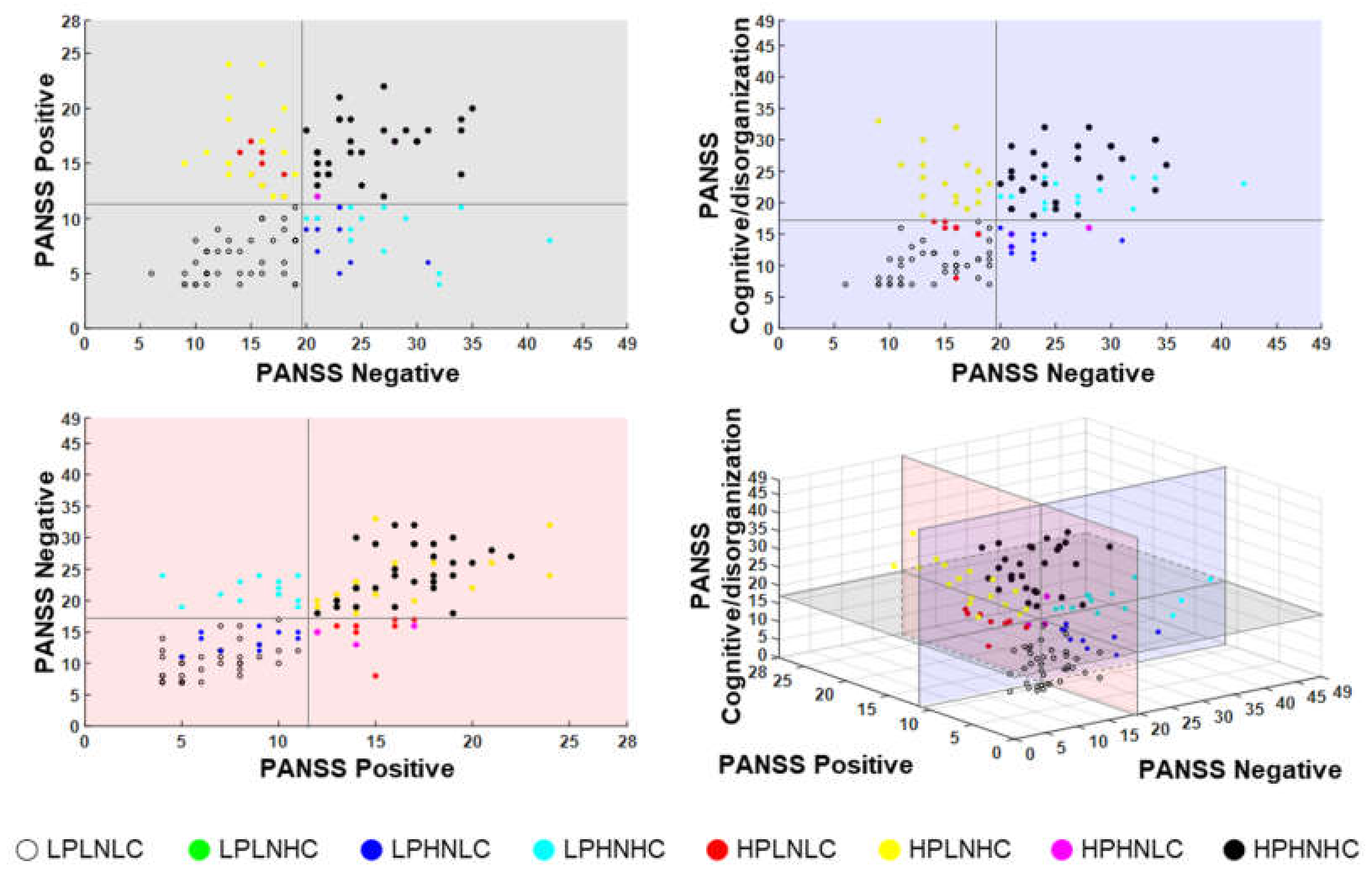
2.2. SZ Subtype Classification according to Symptom Severities
2.3. EEG Data Acquisition and Analysis
2.4. Feature Extraction
2.5. Feature Selection and Classification
3. Results
4. Discussion
Author Contributions
Funding
Conflicts of Interest
References
- American Psychiatric Association. Diagnostic and Statistical Manual of Mental Disorders (DSM-5®); American Psychiatric Publishing: Arlington, VA, USA, 2013. [Google Scholar]
- Lindström, E.; Wieselgren, I.M.; Von Knorring, L. Interrater reliability of the Structured Clinical Interview for the Positive and Negative Syndrome Scale for schizophrenia. Acta Psychiatr. Scand. 1994, 89, 192–195. [Google Scholar] [CrossRef] [PubMed]
- McGorry, P.D.; Mihalopoulos, C.; Henry, L.; Dakis, J.; Jackson, H.J.; Flaum, M.; Harrigan, S.; McKenzie, D.; Kulkarni, J.; Karoly, R. Spurious precision: Procedural validity of diagnostic assessment in psychotic disorders. Am. J. Psychiatry 1995, 152, 220–223. [Google Scholar] [CrossRef] [PubMed]
- Norman, R.M.; Malla, A.K.; Cortese, L.; Diaz, F. A study of the interrelationship between and comparative interrater reliability of the SAPS, SANS and PANSS. Schizophr. Res. 1996, 19, 73–85. [Google Scholar] [CrossRef]
- Winterer, G.; Coppola, R.; Egan, M.F.; Goldberg, T.E.; Weinberger, D.R. Functional and effective frontotemporal connectivity and genetic risk for schizophrenia. Biol. Psychiatry 2003, 54, 1181–1192. [Google Scholar] [CrossRef]
- Lynall, M.-E.; Bassett, D.S.; Kerwin, R.; McKenna, P.J.; Kitzbichler, M.; Muller, U.; Bullmore, E. Functional connectivity and brain networks in schizophrenia. J. Neurosci. 2010, 30, 9477–9487. [Google Scholar] [CrossRef]
- Pae, J.S.; Kwon, J.S.; Youn, T.; Park, H.-J.; Kim, M.S.; Lee, B.; Park, K.S. LORETA imaging of P300 in schizophrenia with individual MRI and 128-channel EEG. Neuroimage 2003, 20, 1552–1560. [Google Scholar] [CrossRef]
- Kawasaki, Y.; Sumiyoshi, T.; Higuchi, Y.; Ito, T.; Takeuchi, M.; Kurachi, M. Voxel-based analysis of P300 electrophysiological topography associated with positive and negative symptoms of schizophrenia. Schizophr. Res. 2007, 94, 164–171. [Google Scholar] [CrossRef]
- Wang, J.; Tang, Y.; Li, C.; Mecklinger, A.; Xiao, Z.; Zhang, M.; Hirayasu, Y.; Hokama, H.; Li, H. Decreased P300 current source density in drug-naive first episode schizophrenics revealed by high density recording. Int. J. Psychophysiol. 2010, 75, 249–257. [Google Scholar] [CrossRef]
- Kim, D.-W.; Shim, M.; Kim, J.-I.; Im, C.-H.; Lee, S.-H. Source activation of P300 correlates with negative symptom severity in patients with schizophrenia. Brain Topogr. 2014, 27, 307–317. [Google Scholar] [CrossRef]
- Kay, S.R.; Sevy, S. Pyramidical model of schizophrenia. Schizophr. Bull. 1990, 16, 537–545. [Google Scholar] [CrossRef]
- Kay, S.R.; Fiszbein, A.; Opler, L.A. The positive and negative syndrome scale (PANSS) for schizophrenia. Schizophr. Bull. 1987, 13, 261–276. [Google Scholar] [CrossRef] [PubMed]
- Strauss, G.P.; Nuñez, A.; Ahmed, A.O.; Barchard, K.A.; Granholm, E.; Kirkpatrick, B.; Gold, J.M.; Allen, D.N. The latent structure of negative symptoms in schizophrenia. JAMA Psychiatry 2018, 75, 1271–1279. [Google Scholar] [CrossRef] [PubMed]
- Mucci, A.; Vignapiano, A.; Bitter, I.; Austin, S.F.; Delouche, C.; Dollfus, S.; Erfurth, A.; Fleischhacker, W.W.; Giordano, G.M.; Gladyshev, I.; et al. A large European, multicenter, multinational validation study of the Brief Negative Symptom Scale. Eur. Neuropsychopharmacol. 2019, 29, 947–959. [Google Scholar] [CrossRef] [PubMed]
- Kirkpatrick, B.; Buchanan, R.W.; McKenny, P.D.; Alphs, L.D.; Carpenter, W.T., Jr. The schedule for the deficit syndrome: An instrument for research in schizophrenia. Psychiatry Res. Neuroimaging 1989, 30, 119–123. [Google Scholar] [CrossRef]
- Bowie, C.R.; Harvey, P.D. Cognitive deficits and functional outcome in schizophrenia. Neuropsych. Dis. Treat. 2006, 2, 531–536. [Google Scholar] [CrossRef] [PubMed]
- Morris, J.C.; Edland, S.; Clark, C.; Galasko, D.; Koss, E.; Mohs, R.; Van Belle, G.; Fillenbaum, G.; Heyman, A. The Consortium to Establish a Registry for Alzheimer’s Disease (CERAD): Part IV. Rates of cognitive change in the longitudinal assessment of probable Alzheimer’s disease. Neurology 1993, 43, 2457. [Google Scholar] [CrossRef]
- Folstein, M.F.; Folstein, S.E.; McHugh, P.R. “Mini-mental state”: A practical method for grading the cognitive state of patients for the clinician. J. Psychiatr. Res. 1975, 12, 189–198. [Google Scholar] [CrossRef]
- Andreasen, N.C. A unitary model of schizophrenia: Bleuler’s fragmented phrene as schizencephaly. Arch. Gen. Psychiat. 1999, 56, 781–787. [Google Scholar] [CrossRef]
- Marder, S.R.; Davis, J.M.; Chouinard, G. The effects of risperidone on the five dimensions of schizophrenia derived by factor analysis: Combined results of the North American trials. J. Clin. Psychiatry 1997. [Google Scholar] [CrossRef]
- Kim, J.-H.; Kim, S.-Y.; Lee, J.; Oh, K.-J.; Kim, Y.-B.; Cho, Z.-H. Evaluation of the factor structure of symptoms in patients with schizophrenia. Psychiatry Res. 2012, 197, 285–289. [Google Scholar] [CrossRef]
- Kay, S.R.; Opler, L.A.; Lindenmayer, J.-P. Reliability and validity of the positive and negative syndrome scale for schizophrenics. Psychiatry Res. 1988, 23, 99–110. [Google Scholar] [CrossRef]
- Bell, M.D.; Lysaker, P.H.; Milstein, R.M.; Beam-Goulet, J.L. Concurrent validity of the cognitive component of schizophrenia: Relationship of PANSS scores to neuropsychological assessments. Psychiatry Res. 1994, 54, 51–58. [Google Scholar] [CrossRef]
- Mortimer, A.M. Symptom rating scales and outcome in schizophrenia. Br. J. Psychiatry 2007, 191, s7–s14. [Google Scholar] [CrossRef] [PubMed]
- Andreasen, N.C. Negative symptoms in schizophrenia: Definition and reliability. Arch. Gen. Psychiatry 1982, 39, 784–788. [Google Scholar] [CrossRef] [PubMed]
- Liemburg, E.; Castelein, S.; Stewart, R.; van der Gaag, M.; Aleman, A.; Knegtering, H.; Outcome of Psychosis (GROUP) Investigators. Two subdomains of negative symptoms in psychotic disorders: Established and confirmed in two large cohorts. J. Psychiatr. Res. 2013, 47, 718–725. [Google Scholar] [CrossRef]
- Lakhan, S.E. Schizophrenia proteomics: Biomarkers on the path to laboratory medicine? Diagn. Pathol. 2006, 1, 11. [Google Scholar] [CrossRef][Green Version]
- Micheloyannis, S.; Pachou, E.; Stam, C.J.; Breakspear, M.; Bitsios, P.; Vourkas, M.; Erimaki, S.; Zervakis, M. Small-world networks and disturbed functional connectivity in schizophrenia. Schizophr. Res. 2006, 87, 60–66. [Google Scholar] [CrossRef]
- Rubinov, M.; Knock, S.A.; Stam, C.J.; Micheloyannis, S.; Harris, A.W.; Williams, L.M.; Breakspear, M. Small-world properties of nonlinear brain activity in schizophrenia. Hum. Brain Mapp. 2009, 30, 403–416. [Google Scholar] [CrossRef]
- Jalili, M.; Knyazeva, M.G. EEG-based functional networks in schizophrenia. Comput. Biol. Med. 2011, 41, 1178–1186. [Google Scholar] [CrossRef]
- Liu, Y.; Liang, M.; Zhou, Y.; He, Y.; Hao, Y.; Song, M.; Yu, C.; Liu, H.; Liu, Z.; Jiang, T. Disrupted small-world networks in schizophrenia. Brain 2008, 131, 945–961. [Google Scholar] [CrossRef]
- Yu, Q.; Sui, J.; Rachakonda, S.; He, H.; Gruner, W.; Pearlson, G.; Kiehl, K.A.; Calhoun, V.D. Altered topological properties of functional network connectivity in schizophrenia during resting state: A small-world brain network study. PLoS ONE 2011, 6, e25423. [Google Scholar] [CrossRef] [PubMed]
- Brady, R.O., Jr.; Gonsalvez, I.; Lee, I.; Öngür, D.; Seidman, L.J.; Schmahmann, J.D.; Eack, S.M.; Keshavan, M.S.; Pascual-Leone, A.; Halko, M.A. Cerebellar-prefrontal network connectivity and negative symptoms in schizophrenia. Am. J. Psychiatry 2019, 176, 512–520. [Google Scholar] [CrossRef] [PubMed]
- Garrity, A.G.; Pearlson, G.D.; McKiernan, K.; Lloyd, D.; Kiehl, K.A.; Calhoun, V.D. Aberrant “default mode” functional connectivity in schizophrenia. Am. J. Psychiatry 2007, 164, 450–457. [Google Scholar] [CrossRef] [PubMed]
- MacDonald, A.W., III; Carter, C.S.; Kerns, J.G.; Ursu, S.; Barch, D.M.; Holmes, A.J.; Stenger, V.A.; Cohen, J.D. Specificity of prefrontal dysfunction and context processing deficits to schizophrenia in never-medicated patients with first-episode psychosis. Am. J. Psychiatry 2005, 162, 475–484. [Google Scholar] [CrossRef]
- Van den Heuvel, M.P.; Mandl, R.C.; Stam, C.J.; Kahn, R.S.; Pol, H.E.H. Aberrant frontal and temporal complex network structure in schizophrenia: A graph theoretical analysis. J. Neurosci. 2010, 30, 15915–15926. [Google Scholar] [CrossRef]
- First, M.B.; Spitzer, R.L.; Gibbon, M.; Williams, J.B. Structured Clinical Interview for DSM-IV Clinical Version (SCID-I/CV); American Psychiatric Press: Washington, DC, USA, 1997. [Google Scholar]
- Yi, J.S.; Ahn, Y.M.; Shin, H.K.; An, S.K.; Joo, Y.H.; Kim, S.H.; Yoon, D.J.; Jho, K.H.; Koo, Y.J.; Lee, J.Y. Reliability and Validity of the Korean Version of the Positive and Negative Syndrome Scale. J. Korean Neuropsychiatr. Assoc. 2001, 40, 1090–1105. [Google Scholar]
- Semlitsch, H.V.; Anderer, P.; Schuster, P.; Presslich, O. A solution for reliable and valid reduction of ocular artifacts, applied to the P300 ERP. Psychophysiology 1986, 23, 695–703. [Google Scholar] [CrossRef]
- Tadel, F.; Baillet, S.; Mosher, J.C.; Pantazis, D.; Leahy, R.M. Brainstorm: A user-friendly application for MEG/EEG analysis. Comput. Intell. Neurosci. 2011, 2011, 879716. [Google Scholar] [CrossRef]
- Destrieux, C.; Fischl, B.; Dale, A.; Halgren, E. Automatic parcellation of human cortical gyri and sulci using standard anatomical nomenclature. Neuroimage 2010, 53, 1–15. [Google Scholar] [CrossRef]
- König, T.; Lehmann, D.; Saito, N.; Kuginuki, T.; Kinoshita, T.; Koukkou, M. Decreased functional connectivity of EEG theta-frequency activity in first-episode, neuroleptic-naıve patients with schizophrenia: Preliminary results. Schizophr. Res. 2001, 50, 55–60. [Google Scholar] [CrossRef]
- Park, Y.-M.; Che, H.-J.; Im, C.-H.; Jung, H.-T.; Bae, S.-M.; Lee, S.-H. Decreased EEG synchronization and its correlation with symptom severity in Alzheimer’s disease. Neurosci. Res. 2008, 62, 112–117. [Google Scholar] [CrossRef] [PubMed]
- Lachaux, J.P.; Rodriguez, E.; Martinerie, J.; Varela, F.J. Measuring phase synchrony in brain signals. Hum. Brain Mapp. 1999, 8, 194–208. [Google Scholar] [CrossRef]
- Pikovsky, A.; Rosenblum, M.; Kurths, J. Synchronization: A Universal Concept in Nonlinear Sciences; Cambridge University Press: Cambridge, UK, 2003; Volume 12. [Google Scholar]
- Rubinov, M.; Sporns, O. Complex network measures of brain connectivity: Uses and interpretations. Neuroimage 2010, 52, 1059–1069. [Google Scholar] [CrossRef] [PubMed]
- Watts, D.J.; Strogatz, S.H. Collective dynamics of ‘small-world’networks. Nature 1998, 393, 440–442. [Google Scholar] [CrossRef]
- Kumar, S.; Sharma, A.; Tsunoda, T. An improved discriminative filter bank selection approach for motor imagery EEG signal classification using mutual information. BMC Bioinform. 2017, 18, 545. [Google Scholar] [CrossRef]
- Amezquita-Garcia, J.A.; Bravo-Zanoguera, M.E.; González-Navarro, F.F.; Lopez-Avitia, R. Hand movement detection from surface electromyography signals by machine learning techniques. In Proceedings of the Latin American Conference on Biomedical Engineering, Cancún, Mexico, 2–5 October 2019; pp. 218–227. [Google Scholar]
- Combrisson, E.; Jerbi, K. Exceeding chance level by chance: The caveat of theoretical chance levels in brain signal classification and statistical assessment of decoding accuracy. J. Neurosci. Methods 2015, 250, 126–136. [Google Scholar] [CrossRef]
- Chyzhyk, D.; Grana, M.; Öngür, D.; Shinn, A.K. Discrimination of schizophrenia auditory hallucinators by machine learning of resting-state functional MRI. Int. J. Neural Syst. 2015, 25, 1550007. [Google Scholar] [CrossRef]
- Peters, H.; Shao, J.; Scherr, M.; Schwerthöffer, D.; Zimmer, C.; Förstl, H.; Bäuml, J.; Wohlschläger, A.; Riedl, V.; Koch, K. More consistently altered connectivity patterns for cerebellum and medial temporal lobes than for amygdala and striatum in schizophrenia. Front. Hum. Neurosci. 2016, 10, 55. [Google Scholar] [CrossRef]
- Guo, W.; Liu, F.; Chen, J.; Wu, R.; Li, L.; Zhang, Z.; Zhao, J. Family-based case-control study of homotopic connectivity in first-episode, drug-naive schizophrenia at rest. Sci. Rep. 2017, 7, 43312. [Google Scholar] [CrossRef]
- Phang, C.-R.; Noman, F.; Hussain, H.; Ting, C.-M.; Ombao, H. A multi-domain connectome convolutional neural network for identifying schizophrenia from EEG connectivity patterns. IEEE J. Biomed. Health Inform. 2019, 24, 1333–1343. [Google Scholar] [CrossRef]
- Anticevic, A.; Cole, M.W.; Repovs, G.; Murray, J.D.; Brumbaugh, M.S.; Winkler, A.M.; Savic, A.; Krystal, J.H.; Pearlson, G.D.; Glahn, D.C. Characterizing thalamo-cortical disturbances in schizophrenia and bipolar illness. Cereb. Cortex 2014, 24, 3116–3130. [Google Scholar] [CrossRef] [PubMed]
- Watanabe, T.; Kessler, D.; Scott, C.; Angstadt, M.; Sripada, C. Disease prediction based on functional connectomes using a scalable and spatially-informed support vector machine. Neuroimage 2014, 96, 183–202. [Google Scholar] [CrossRef] [PubMed]
- Cabral, C.; Kambeitz-Ilankovic, L.; Kambeitz, J.; Calhoun, V.D.; Dwyer, D.B.; Von Saldern, S.; Urquijo, M.F.; Falkai, P.; Koutsouleris, N. Classifying schizophrenia using multimodal multivariate pattern recognition analysis: Evaluating the impact of individual clinical profiles on the neurodiagnostic performance. Schizophr. Bull. 2016, 42, S110–S117. [Google Scholar] [CrossRef] [PubMed]
- Iwabuchi, S.J.; Palaniyappan, L. Abnormalities in the effective connectivity of visuothalamic circuitry in schizophrenia. Psychol. Med. 2017, 47, 1300. [Google Scholar] [CrossRef]
- Schnack, H.G.; Kahn, R.S. Detecting neuroimaging biomarkers for psychiatric disorders: Sample size matters. Front. Psychiatry 2016, 7, 50. [Google Scholar] [CrossRef]
- Barabassy, A.; Szatmári, B.; Laszlovszky, I.; Németh, G. Negative symptoms of schizophrenia: Constructs, burden, and management. In Psychotic Disorders—An Update; Durbano, F., Ed.; Intech Open: London, UK, 2018. [Google Scholar]
- Sadock, B.; Sadock, V.; Ruiz, P. Kaplan and Sadock’s Synopsis of Psychiatry: Behavioral Sciences/Clinical Psychiatry; Wolters Kluwer: Philadelphia, PA, USA, 2014. [Google Scholar]
- Slifstein, M.; Van De Giessen, E.; Van Snellenberg, J.; Thompson, J.L.; Narendran, R.; Gil, R.; Hackett, E.; Girgis, R.; Ojeil, N.; Moore, H. Deficits in prefrontal cortical and extrastriatal dopamine release in schizophrenia: A positron emission tomographic functional magnetic resonance imaging study. JAMA Psychiatry 2015, 72, 316–324. [Google Scholar] [CrossRef]
- Clementz, B.A.; Grove, W.M.; Katsanis, J.; Iacono, W.G. Psychometric detection of schizotypy: Perceptual aberration and physical anhedonia in relatives of schizophrenics. J. Abnorm. Psychol. 1991, 100, 607. [Google Scholar] [CrossRef]
- Keefe, R.S.; Lobelc, D.S.; Mohs, R.C.; Silverman, J.M.; Harvey, P.D.; Davidson, M.; Losonczy, M.F.; Davis, K.L. Diagnostic issues in chronic schizophrenia: Kraepelinian schizophrenia, undifferentiated schizophrenia, and state-independent negative symptoms. Schizophr. Res. 1991, 4, 71–79. [Google Scholar] [CrossRef]
- Berenbaum, H.; McGrew, J. Familial resemblance of schizotypic traits. Psychol. Med. 1993, 23, 327–333. [Google Scholar] [CrossRef]
- Rey, E.R.; Bailer, J.; Bräuer, W.; Händel, M.; Laubenstein, D.; Stein, A. Stability trends and longitudinal correlations of negative and positive syndromes within a three-year follow-up of initially hospitalized schizophrenics. Acta Psychiatr. Scand. 1994, 90, 405–412. [Google Scholar] [CrossRef]
- Dollfus, S.; Petit, M. Negative symptoms in schizophrenia: Their evolution during an acute phase. Schizophr. Res. 1995, 17, 187–194. [Google Scholar] [CrossRef]
- Lyons, M.J.; Toomey, R.; Faraone, S.V.; Kremen, W.S.; Yeung, A.S.; Tsuang, M.T. Correlates of psychosis proneness in relatives of schizophrenic patients. J. Abnorm. Psychol. 1995, 104, 390. [Google Scholar] [CrossRef] [PubMed]
- Blanchard, J.J.; Mueser, K.T.; Bellack, A.S. Anhedonia, positive and negative affect, and social functioning in schizophrenia. Schizophr. Bull. 1998, 24, 413–424. [Google Scholar] [CrossRef] [PubMed]
- Fusar-Poli, P.; Papanastasiou, E.; Stahl, D.; Rocchetti, M.; Carpenter, W.; Shergill, S.; McGuire, P. Treatments of negative symptoms in schizophrenia: Meta-analysis of 168 randomized placebo-controlled trials. Schizophr. Bull. 2015, 41, 892–899. [Google Scholar] [CrossRef] [PubMed]
- Wang, L.; Zou, F.; Shao, Y.; Ye, E.; Jin, X.; Tan, S.; Hu, D.; Yang, Z. Disruptive changes of cerebellar functional connectivity with the default mode network in schizophrenia. Schizophr. Res. 2014, 160, 67–72. [Google Scholar] [CrossRef] [PubMed]
- Duan, H.-F.; Gan, J.-L.; Yang, J.-M.; Cheng, Z.-X.; Gao, C.-Y.; Shi, Z.-J.; Zhu, X.-Q.; Liang, X.-J.; Zhao, L.-M. A longitudinal study on intrinsic connectivity of hippocampus associated with positive symptom in first-episode schizophrenia. Behav. Brain Res. 2015, 283, 78–86. [Google Scholar] [CrossRef]
- Tang, Y.; Chen, K.; Zhou, Y.; Liu, J.; Wang, Y.; Driesen, N.; Edmiston, E.K.; Chen, X.; Jiang, X.; Kong, L. Neural activity changes in unaffected children of patients with schizophrenia: A resting-state fMRI study. Schizophr. Res. 2015, 168, 360–365. [Google Scholar] [CrossRef]
- Xu, Y.; Zhuo, C.; Qin, W.; Zhu, J.; Yu, C. Altered spontaneous brain activity in schizophrenia: A meta-analysis and a large-sample study. BioMed Res. Int. 2015, 2015, 204628. [Google Scholar] [CrossRef]
- Zhou, Y.; Ma, X.; Wang, D.; Qin, W.; Zhu, J.; Zhuo, C.; Yu, C. The selective impairment of resting-state functional connectivity of the lateral subregion of the frontal pole in schizophrenia. PLoS ONE 2015, 10, e0119176. [Google Scholar] [CrossRef]
- Fujiki, R.; Morita, K.; Sato, M.; Yamashita, Y.; Kato, Y.; Ishii, Y.; Shoji, Y.; Uchimura, N. Single event-related changes in cerebral oxygenated hemoglobin using word game in schizophrenia. Neuropsychiatr. Dis. Treat 2014, 10, 2353. [Google Scholar] [CrossRef]
- Watanabe, A.; Kato, T. Cerebrovascular response to cognitive tasks in patients with schizophrenia measured by near-infrared spectroscopy. Schizophr. Bull. 2004, 30, 435–444. [Google Scholar] [CrossRef] [PubMed]
- Ehlis, A.-C.; Herrmann, M.J.; Plichta, M.M.; Fallgatter, A.J. Cortical activation during two verbal fluency tasks in schizophrenic patients and healthy controls as assessed by multi-channel near-infrared spectroscopy. Psychiatry Res. Neuroimaging 2007, 156, 1–13. [Google Scholar] [CrossRef] [PubMed]
- Mitchell, A.C.; Jiang, Y.; Peter, C.; Akbarian, S. Transcriptional regulation of GAD1 GABA synthesis gene in the prefrontal cortex of subjects with schizophrenia. Schizophr. Res. 2015, 167, 28–34. [Google Scholar] [CrossRef]
- Culham, J.C.; Kanwisher, N.G. Neuroimaging of cognitive functions in human parietal cortex. Curr. Opin. Neurobiol. 2001, 11, 157–163. [Google Scholar] [CrossRef]


| SZ (n = 119) | NC (n = 119) | p-Value | |
|---|---|---|---|
| Mean ± SD or n | |||
| Age (years) | 36.26 ± 12.40 | 36.67 ± 11.66 | 0.792 |
| Sex | 0.794 | ||
| Male | 53 | 51 | |
| Female | 66 | 68 | |
| Education (years) | 13.05 ± 2.89 | 13.55 ± 2.89 | 0.186 |
| Number of hospitalization | 2.43 ± 2.88 | ||
| Duration of illness (years) | 9.93 ± 9.21 | ||
| Dosage of antipsychotics (chlorpromazine equivalent, mg) | 887.83 ± 1110.95 | ||
| Positive and negative syndrome scale (PANSS) | |||
| Positive | 19.21 ± 8.69 | ||
| Negative | 19.93 ± 6.66 | ||
| General | 41.75 ± 13.80 | ||
| Total | 80.89 ± 25.31 | ||
| Five-factor model of the PANSS | |||
| Positive | 11.56 ± 5.26 | ||
| Negative | 19.60 ± 6.95 | ||
| Cognitive/disorganization | 17.69 ± 7.16 | ||
| Excitement | 12.72 ± 5.86 | ||
| Depression/anxiety | 11.79 ± 3.84 | ||
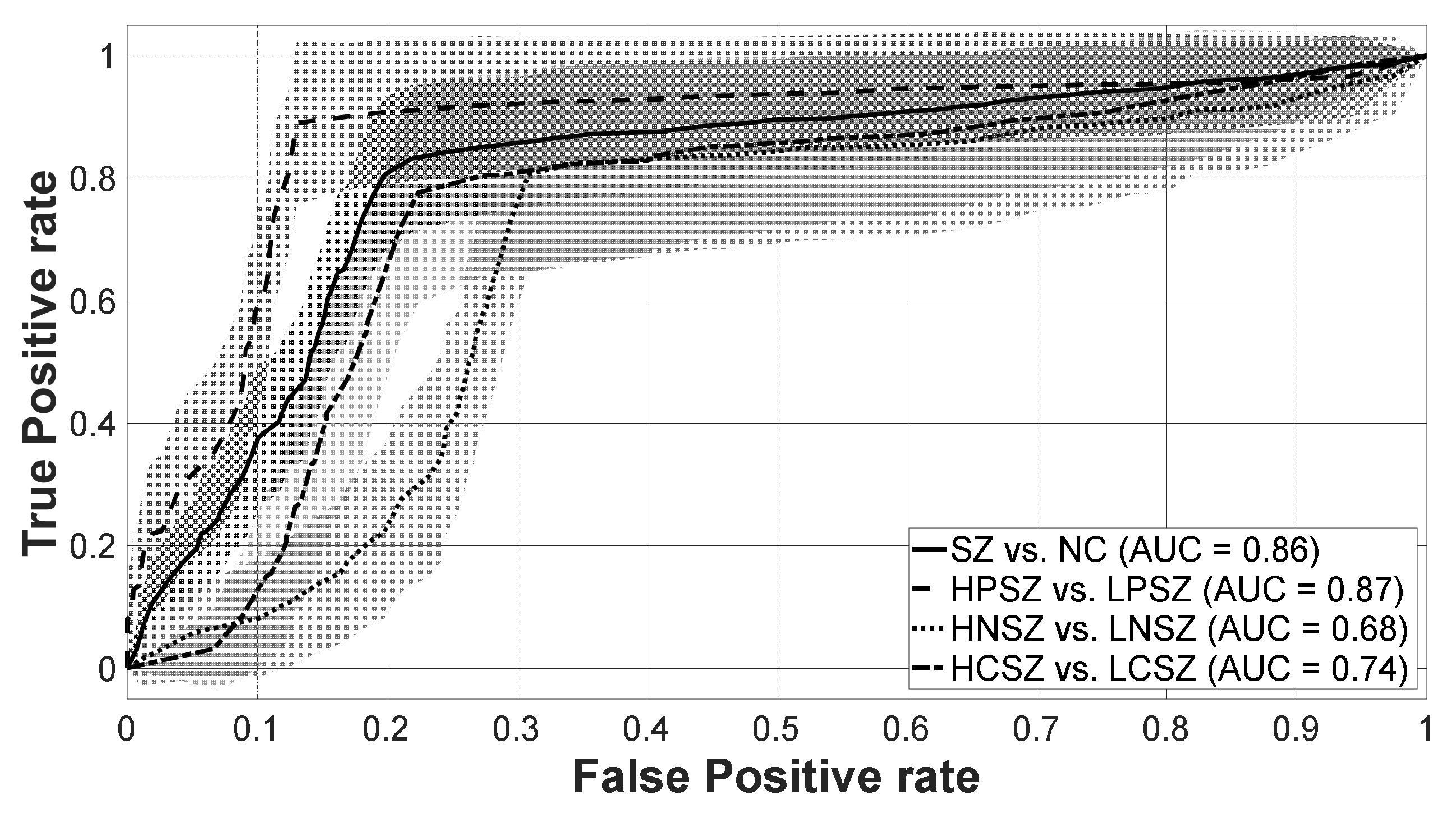
| Two-Classes Classification | Accuracy (%) | Sensitivity (%) | Specificity (%) | # of Features | |||||||
|---|---|---|---|---|---|---|---|---|---|---|---|
| SZ (n = 119) vs. NC (n = 119) | 80.66 | 78.83 | 82.48 | 27 | |||||||
| HPSZ (n = 57) vs. LPSZ (n = 62) | 88.10 | 88.40 | 87.77 | 19 | |||||||
| HNSZ (n = 55) vs. LNSZ (n = 64) | 75.25 | 80.76 | 68.50 | 7 | |||||||
| HCSZ (n = 59) vs. LCSZ (n = 60) | 77.78 | 77.83 | 77.80 | 27 | |||||||
| Selected features ranking (brain region) | 1st | 2nd | 3rd | 4th | 5th | ||||||
| SZ vs. NC | Frontal | > | Occipital | > | Limbic | > | Temporal | = | Parietal | ||
| HPSZ vs. LPSZ | Frontal | > | Tempo-Occipital | > | Temporal | = | Occipital | = | Parietal | ||
| HNSZ vs. LNSZ | Frontal | = | Tempo-Occipital | = | Parietal | > | Insula | ||||
| HCSZ vs. LCSZ | Parietal | > | Frontal | > | Temporal | = | Limbic | ||||
| Selected features ranking (frequency band) | 1st | 2nd | 3rd | 4th | 5th | 6th | |||||
| SZ vs. NC | Theta | = | Beta3 | > | Delta | > | Alpha | > | Beta2 | ||
| HPSZ vs. LPSZ | Alpha | > | Delta | > | Theta | = | Alpha1 | = | Beta4 | = | gamma |
| HNSZ vs. LNSZ | Alpha2 | > | Delta | = | Theta | = | Beta1 | = | Beta4 | = | gamma |
| HCSZ vs. LCSZ | Beta2 | > | Delta | = | Alpha | = | Beta | > | Gamma | ||
| # | Accuracy (%) | Sensitivity (%) | Specificity (%) | Frequency Band | Brain Region |
|---|---|---|---|---|---|
| 1 | 63.69 | 70.52 | 56.03 | Delta | Supramarginal gyrus R |
| 2 | 69.83 | 75.98 | 62.60 | Alpha2 | Anterior transverse collateral sulcus L |
| 3 | 71.99 | 76.38 | 66.90 | Gamma | Precuneus (medial part of P1) R |
| 4 | 73.90 | 80.05 | 67.10 | Beta1 | Inferior segment of the circular sulcus of the insula L |
| 5 | 74.67 | 80.81 | 67.33 | Theta | Posterior transverse collateral sulcus L |
| 6 | 75.13 | 80.33 | 68.93 | Alpha2 | Triangular part of the inferior frontal gyrus L |
| 7 | 75.25 | 80.76 | 68.50 | Beta4 | Marginal branch (or part) of the cingulate sulcus R |
Publisher’s Note: MDPI stays neutral with regard to jurisdictional claims in published maps and institutional affiliations. |
© 2020 by the authors. Licensee MDPI, Basel, Switzerland. This article is an open access article distributed under the terms and conditions of the Creative Commons Attribution (CC BY) license (http://creativecommons.org/licenses/by/4.0/).
Share and Cite
Kim, J.-Y.; Lee, H.S.; Lee, S.-H. EEG Source Network for the Diagnosis of Schizophrenia and the Identification of Subtypes Based on Symptom Severity—A Machine Learning Approach. J. Clin. Med. 2020, 9, 3934. https://doi.org/10.3390/jcm9123934
Kim J-Y, Lee HS, Lee S-H. EEG Source Network for the Diagnosis of Schizophrenia and the Identification of Subtypes Based on Symptom Severity—A Machine Learning Approach. Journal of Clinical Medicine. 2020; 9(12):3934. https://doi.org/10.3390/jcm9123934
Chicago/Turabian StyleKim, Jeong-Youn, Hyun Seo Lee, and Seung-Hwan Lee. 2020. "EEG Source Network for the Diagnosis of Schizophrenia and the Identification of Subtypes Based on Symptom Severity—A Machine Learning Approach" Journal of Clinical Medicine 9, no. 12: 3934. https://doi.org/10.3390/jcm9123934
APA StyleKim, J.-Y., Lee, H. S., & Lee, S.-H. (2020). EEG Source Network for the Diagnosis of Schizophrenia and the Identification of Subtypes Based on Symptom Severity—A Machine Learning Approach. Journal of Clinical Medicine, 9(12), 3934. https://doi.org/10.3390/jcm9123934