3.1. Effect of the Body-Generated Vortices
The body of the fish model is composed of the stationary head, stationary sting, and pitching tail section. Each component generates a boundary layer and has the potential to generate vortices that can interact with the caudal fin downstream. The Q-criterion, also referred to as
Q, is an Eulerian scalar used for vortex identification as proposed by Hunt et al., and its definition is shown in Equation (
3). The velocity gradient tensor,
, can be decomposed such that
, where
is the symmetric rate of strain tensor and
is the anti-symmetric rate of rotation tensor.
represents the Euclidean (Frobenius) norm of
.
Any region with values of
Q larger than zero are regions where the local rate of rotation,
, is dominant over the local rate of strain,
S [
44]. In
Figure 6,
Figure 7,
Figure 8 and
Figure 9, the lowest contour is set to
, which is approximately
of the global maximum value. The value is set above zero to eliminate experimental noise in the visualization.
Figure 6A shows the wake beside the body and caudal fin at the midspan plane (0 mm) for case 8 (
,
). There are several small structures forming in the boundary layer of the tail, but none of these structures are strong enough to persist downstream and interact with the caudal fin.
Figure 6B shows the wake between the body and caudal fin at the
mm plane. Small structures in the boundary layer are also visible in this plane, but none of them persist long enough to interact with the caudal fin.
Figure 6C shows the wake between the body and caudal fin at the
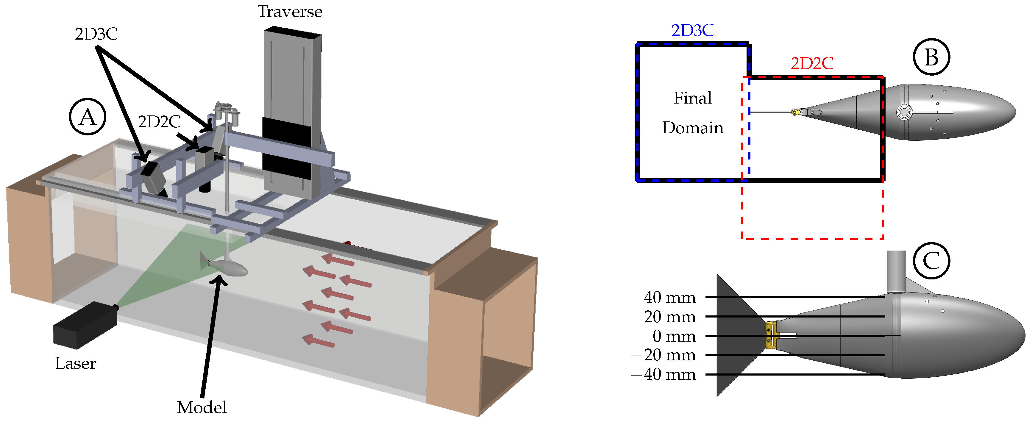
mm plane. We believe that the vortices shown here are generated by the sting, and they appear to dissipate in the flow before being able to interact with the caudal fin as discrete vortices. The sting did generate more turbulence in the flow that caused more uncertainty in the phase-averaged data. For this reason, the two negative planes are used in future sections to describe the flow at the
mm and
mm planes. The flow between the body and caudal fin could not be observed below the midspan plane due to the body shadow (
mm and
mm planes). Overall, the body-generated vortices are not strong enough to persist in the flow and interact with the caudal fin. This is in agreement with the recent numerical work by Liu et al., who observed that the body-generated vortices of a crevalle jack fish without the dorsal/ventral fins were not strong enough to interact with the caudal fin in a meaningful way [
22]. Observations described here are consistent across all eight cases.
3.2. Leading Edge Vortex Formation
As the fin moves relative to the surrounding fluid, a shear layer forms along each edge of the fin as fluid flows around the edge. We refer to the anterior swept edge of the caudal fin as the leading edge, and a vortex that forms along this edge as a leading edge vortex (LEV). Borazjani and Dghooghi [
24] and Liu et al. [
22] have previously identified LEVs forming on the caudal fin of carangiform swimmers. Our results are consistent with those, identifying LEVs using
Q at the
mm plane (
Figure 7) and
mm plane (
Figure 8). We only present the planes below the midspan (
) as they are less affected by the wake of the sting. The LEVs described here are on the
side of the fin, which is not in the shadow of either the fin or the body/tail. The 0 mm plane does not form an LEV because the body connects to the fin in this region (
), eliminating the leading edge.
During each half-cycle, an LEV forms along the swept leading edge of the fin due to a shear layer whose strength is proportional to the edge’s velocity relative to the surrounding fluid. For all cases, the edge’s velocity is smallest at the peduncle joint and increases along the chord of the rigid fin. This creates an LEV with nonuniform circulation that is weakest at the peduncle joint and strongest near the spanwise tips. Buchholz and Smits [
7] linked a nonuniform chordwise edge vortex to a chordwise pressure gradient on the surface of the fin. Simply for illustrative purposes, we use case 7 as an example here to describe the life-cycle of an LEV forming on the caudal fin. Videos of all eight cases for the
mm and
mm planes (where applicable) are available in
Supplementary Videos S1 through S14. The
mm and
mm planes are shown in
Figure 7 and
Figure 8, respectively.
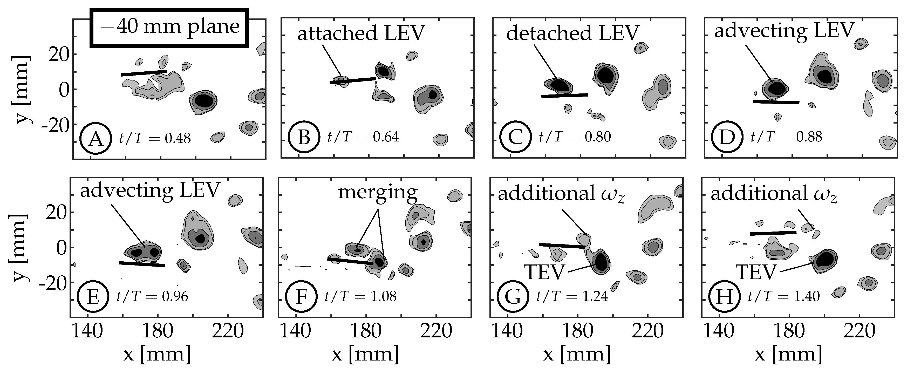
The example starts at
with the caudal fin at the positive amplitude extreme and starting to move downward (between
Figure 7A,B). The LEV forms at
and can be seen in
Figure 7B (
). It continues to grow in size and strength until
(
Figure 7C). The relative strength of LEVs is determined using
Q contours to compare the size and magnitudes within the structures. If two structures have similar
Q values throughout and one is larger than the other, we infer that the larger structure contains more circulation and is considered “stronger”. Similarly, if two structures have similar size and one has higher peak magnitudes of
Q, then the structure with higher
Q magnitudes is assumed to contain more circulation and is considered stronger. At
(
Figure 7C), the LEV has already detached from the surface at the
mm planes, but remains attached at the
mm planes (compare
Figure 7C and
Figure 8C). We consider the LEV to no longer be attached if a gap is present between the lowest contour level and the fin. At the
mm planes, the shear layer feeding the vortex is pinched-off between
and
, allowing the shed LEV to advect along the fin (
Figure 7D,E) and eventually merge with the forming trailing edge vortex (TEV) of the same sign (
,
Figure 7F). After the merging, the trailing edge continues to move upward generating additional vorticity that is not entrained in the primary vortex (
Figure 7G,H). At the
mm planes, the LEV remains attached (
Figure 8C–E) and does not appear to advect along the fin. Instead, it dissipates, or is swept back around the leading edge as an LEV is formed on the opposite side during the next half-cycle (
Figure 8F–H). Some combination of these two behaviors is also possible.
A few trends are observed across the four kinematic groups. The first is a result of the fact that the relative velocity of the leading edge, for a given nondimensional time and distance from the fin’s pitching axis, obviously increases with maximum tail amplitude (
) as this angle is related to the motion of the peduncle. The size and strength of the LEV increases accordingly as can be seen in
Figure 9 (both
mm and
mm planes). In these plots, case 5 (
Figure 9A,E) has the smallest LEV and case 8 (
Figure 9D,H) has the largest LEV.
Second, the numerical investigation of crevalle jack fish with video-captured geometry and kinematics by Liu et al., observed that the entire LEV was advected along the fin chord and merged with the TEV. In the current work, and for all cases, this behavior is only observed at the
mm planes while the LEV at the
mm planes appears to dissipate, is swept back across the leading edge, or some combination of these two. For all cases at the
mm planes, the LEV begins to merge with the TEV around the same nondimensional time (
) and continues through
(mid-merge is shown in
Figure 7F).
Third, with increasing maximum tail amplitude the LEV forms along the entire leading edge earlier in the half-cycle. At the
mm planes, the LEV also detaches from the surface earlier in the half-cycle with increasing maximum tail amplitude. For cases 5 and 6, the LEV detaches from the surface between
and
. For cases 7 and 8, which have larger tail amplitude, the detachment occurs between
and
. The top row of
Figure 9 shows that at
, the LEVs in cases 5 and 6 are still attached (
Figure 9A,B) while in cases 7 and 8, they are already detached (
Figure 9C,D). We note here that in general, the relative velocity of the leading edge and the strength of the resulting LEV would decrease as phase offset between tail and caudal fin motion (
) increased from
to
, if TE amplitude (
A) were kept constant.
The numerical simulations by Liu et al., linked the presence of attached LEVs to peaks in thrust, showing the significance of LEVs in the generation of thrust [
22]. The data shown in the current work suggests that the phenomenon of LEV attachment and detachment is also related to the leading edge velocity, which is governed by the body-fin kinematic parameters (
,
, and
). We acknowledge that the kinematic discrepancy (discussed in
Section 2.2) may have an effect on the formation and shedding of the LEVs, but the connection has not been determined. We believe that the link is less obvious because only one LEV is formed per half-cycle unlike the TEV where multiple vortices are shed per half-cycle.
3.3. Circulation Production in the Wake
The amount of circulation generated per half-cycle at the midspan in these experiments is similar among cases with similar kinematics despite having different freestream velocities. This supports the hypothesis that the magnitude of circulation production is insensitive to freestream velocity as proposed by Buchholz et al. [
45]. The first and second Strouhal number groups have a nominal Strouhal number (
) of
and
, respectively. In our experiments,
was varied to change
. Within each Strouhal number group,
varies slightly due to experimental variation in
A; but between the two groups, the freestream velocity is the dominant distinguishing parameter.
A time history of circulation produced by the trailing edge at the midspan was calculated by considering a rectangular region downstream of the TE. The region is tall enough to capture the full transverse extent of the wake and extends far enough downstream to contain the total amount of circulation shed in one half-cycle. To do this, the upstream and transverse boundaries of the region are held stationary while the downstream boundary moves with the approximate vortex advection speed. Case 5 is used in
Figure 10 as an illustrative example for the method of calculating the circulation history. This figure shows the first phase with vorticity present (
Figure 10A,
), the phase with peak circulation (
Figure 10B,
), and a later phase (
Figure 10C,
) once positive (red) vorticity is no longer being generated. The phase
is before the half-cycle begins and it is shown because it is the beginning of vorticity generation for the given half-cycle. Each half-cycle is defined by the trailing edge reaching an amplitude maximum or minimum. An area integral of the vorticity magnitude above a threshold of
within the region was used to calculate the circulation, and the time history of positive and negative circulation for this case can be seen in
Figure 11B as the solid red and blue curves, respectively. The positive and negative circulation time histories for the other seven cases are shown in
Figure 11B through
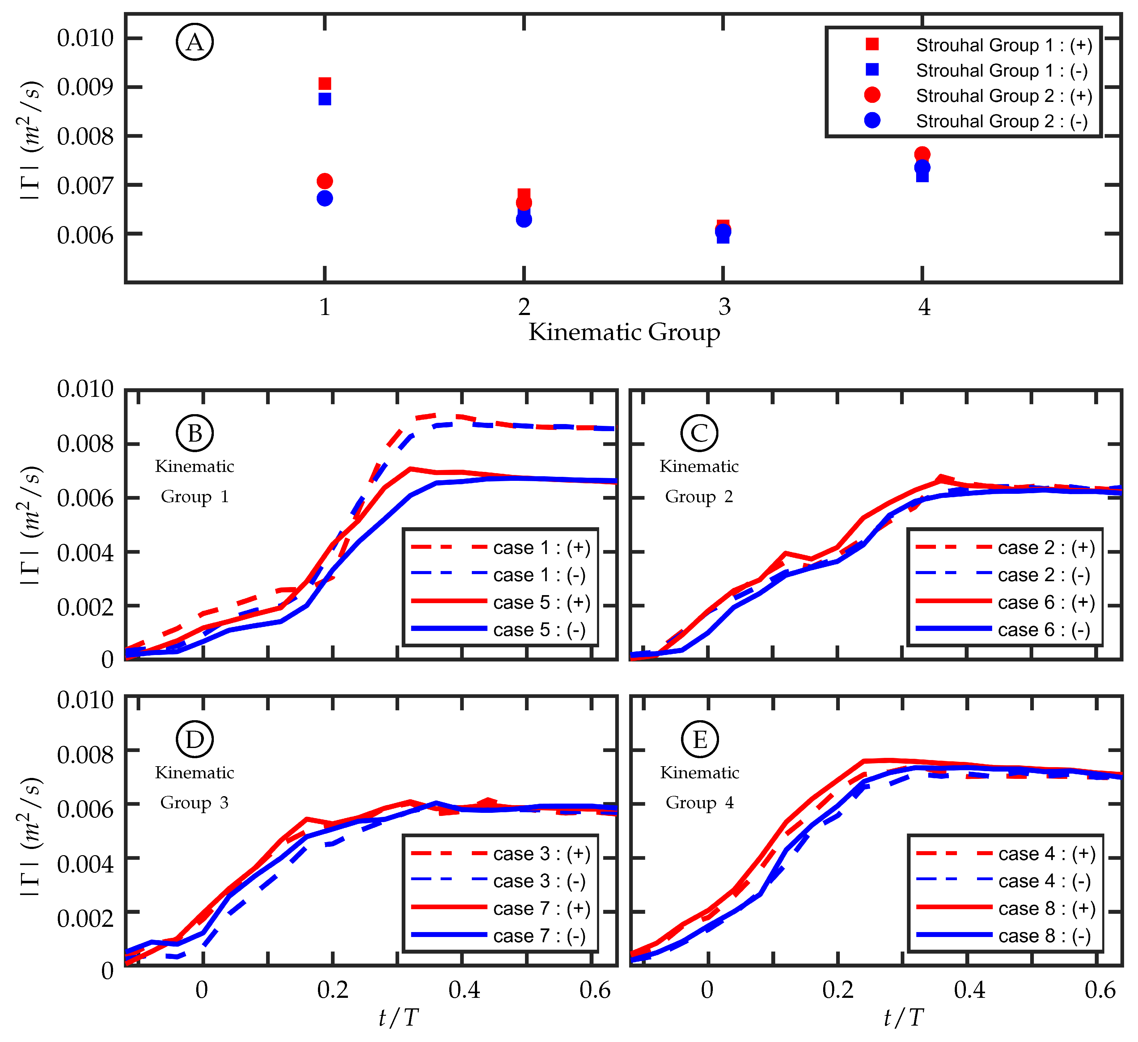
Figure 11E. For each case, the circulation rises during the beginning of the half-cycle, reaches a maximum value, and then plateaus. The plateau indicates that the amount of circulation, of that sign, remains relatively constant with a slow decrease due to viscous dissipation and interaction with neighboring structures. The maximum value at the beginning of the plateau region is considered the total circulation produced during that half-cycle.
For each time history (
Figure 11B through
Figure 11E), the positive and negative circulation produced per half-cycle match reasonably well with some variation during the beginning of the half-cycle. The consistency supports experimental symmetry. The maximum circulations produced per half-cycle within each kinematic group are compared in
Figure 11A, and the values align well for kinematic groups 2, 3, and 4. Kinematic group 1 does not match as well between the two Strouhal numbers. One possible explanation for this is that the motion profile in kinematic group 1 is characterized by entirely caudal fin motion and, as discussed in
Section 2.2, the kinematic discrepancy is most noticeable in this motion.
The discrepancy-caused variation in the trailing edge amplitude,
A, among all cases was summarized in
Table 1. In each kinematic group, this resulted in a difference between the two
cases, but it was not always true that the larger
A corresponded to the higher
(recalling that
was set by adjusting the freestream velocity and nominally holding
A constant). In kinematic groups 2, 3, and 4, the larger trailing edge amplitude between the two cases was 5.7%, 6.4%, and 1.8% higher than the lower one, respectively, while for kinematic group 1 the difference was
. Of this kinematic group, case 1 (dashed lines) and case 5 (solid lines) are shown in
Figure 11B. Despite its lower
, case 1, which had
mm, had a larger trailing edge amplitude and produced more circulation than case 5, which had
mm. The differences of
A between the cases in kinematic groups 2, 3, and 4 are smaller than in kinematic group 1, and the time histories of circulation produced are more similar. The fact that there is
not a large difference between the cases in kinematic groups 2, 3, and 4 indicates that the amount of circulation produced per half-cycle is relatively insensitive to freestream velocity. The large difference in circulation produced between cases 1 and 5 suggests that circulation production is sensitive to
A and by extension trailing edge velocity. The pitching frequency (
f) is held constant for all cases so an increase in
A corresponds to an increase in trailing edge velocity.
3.4. Effect of Nonsinusoidal Trailing Edge Kinematics
The vorticity in the wake of the fish model is arranged in a series of vortices that each originates in a shear layer created by the relative motion of the caudal fin trailing edge (TE) and the surrounding fluid. For this reason, the generation and arrangement of vorticity in the wake behind this two degree-of-freedom model is sensitive to the trailing edge kinematics. The experimental data is composed of four kinematic groups, which result in four distinct wake structures. Each will be explained in relation to their TE kinematics. Cases 1 and 4 will be discussed in more depth to exemplify the differences between a square-like (case 1) and a sinusoidal (case 4) waveform.
The TE amplitude is held relatively constant in cases 2 through 4 while case 1 has a TE amplitude that is larger due to experimental error. Despite this, the main difference between the cases is the amount of the TE amplitude that is contributed by either the tail or the caudal fin. To better understand how this affects the motion waveform we consider a simple example (
Figure 12) of adding two sinusoids (a model tail motion
T, dotted curve, and a model caudal fin motion
C, dashed curve) with a fixed offset between them (
) that results in a third sinusoid (the trailing edge excursion
A, solid curve). The vertical lines in the figure represent the timing of each peak.
is equal to the distance between the vertical dashed and dotted lines, and is the same in both figures. The phase offset between the model resultant curve (
A) and the model caudal fin curve (
C) is the distance between the vertical solid and dashed lines.
Figure 12 shows two examples where the resultant curves (
A) have the same peak amplitude. In
Figure 12A, the majority of
A is from
T; while in
Figure 12B, the majority of
A is from
C. From these examples, we can see that the phase offset between
C and
A is dependent on the relative peak amplitudes of
T and
C. In the experiments, the phase offset between the tail and caudal fin motion (
) is fixed at
and the TE excursion is fixed at approximately 22 mm, but the phase offset between the caudal fin and the TE motion thus varies. The actual waveform of the caudal fin in our experiments is square-like due to the kinematic discrepancy. This additionally causes the waveform of the TE motion to vary depending on how much of the amplitude is contributed by the caudal fin. Both effects are observed to have a significant impact on the vorticity generated at the trailing edge.
The actual experimental waveforms can be seen in
Figure 13. In this figure, the TE amplitude is represented by the solid curve and the TE velocity is represented by the dashed curve. These curves are overlaid with colored regions representing time periods of TE acceleration (red) and TE deceleration (blue) as well as yellow circles representing the approximate timing of vortex shedding. The diameter of the circles is equal to the temporal resolution of the dataset. Due to the discrete nature of experimental data, we are unable to pinpoint the exact timing of events, but we can identify a time period during which the event took place. For the purposes of this discussion, the yellow circles will be identified by the center time that occurs between the experimental time steps.
Figure 14 shows the vorticity arrangement for cases 1 through 4 at
. In cases 1 through 3, the primary vortices (P1 and P2) are shed during periods of TE deceleration; while in case 4, the primary vortex is shed during a period when the TE is still accelerating. This suggests that two different shedding mechanisms may be involved. In case 1, the TE is weakly accelerating between
and
(
Figure 13A). During this time period, the TE is nearly stationary as previously described and results in a weak shear layer that rolls up into discrete vortices due to what we assume are general shear layer instabilities. These early vortices will be referred to as secondary vortices (S1, S2, etc.). The primary vortex grows during a period of TE acceleration (
) and is shed at
during a period of TE deceleration. The full half-cycle can be seen in
Figure 15 and the vorticity arrangement at the end of the half-cycle can be see in
Figure 14A. In case 2, the first primary vortex (P1) is formed during a period of TE acceleration (
) and is shed at
. The second primary vortex (P2) is also formed during a period of TE acceleration (
) and is shed at
. Both vortices are shed during periods of TE deceleration (
Figure 13B and
Figure 14B). In case 3, the first primary vortex (P1) is formed during a period of TE acceleration (
) and is shed at
. The second primary vortex (P2) is also formed during a period of TE acceleration (
) and is shed at
. Both vortices are shed during periods of TE deceleration (
Figure 13C and
Figure 14C). In case 4, the primary vortex (P1) is formed during a period of TE acceleration (
) and is shed at
while the remaining shear layer rolls up into trailing secondary vortices (S1 and S2). Unlike the previous three cases where the primary vortices are shed during periods of TE deceleration, the primary vortex in this case is shed during the initial period of TE acceleration. The full half-cycle can be seen in
Figure 16. In cases 1 through 3, the deceleration of the TE results in the shedding of a forming vortex while in case 4 we believe the vortex becomes saturated and subsequently sheds during a period of TE acceleration. The mechanism in case 4 may be consistent with DeVoria and Ringuette who suggested that a steadily forming vortex will shed once it has become saturated and any remaining circulation is collected into a series of small vortices in the wake of the primary vortex [
46].
A second trend in cases 1 through 4 concerns the distribution of vorticity between the vortices that are shed per half-cycle. In case 1, The TE motion is entirely a result of the caudal fin and the wake consists of a weaker first vortex and a stronger second vortex. As tail motion is added, the first vortex becomes stronger and the second vortex becomes weaker. This is seen in cases 2 and 3 where the case 2 wake has two vortices of similar strength and case 3 has a stronger first vortex and a weaker second vortex. We hypothesize that if more cases are generated between these cases a clear transition will be observed. This transition may not be caused by the addition of tail motion itself, but is more likely the result of two factors: the short periods of deceleration due to the kinematic discrepancy, which weakens as the motion shifts from all caudal fin contribution to all tail contribution; as well as the changing phase offset between the total TE motion and the caudal fin motion.
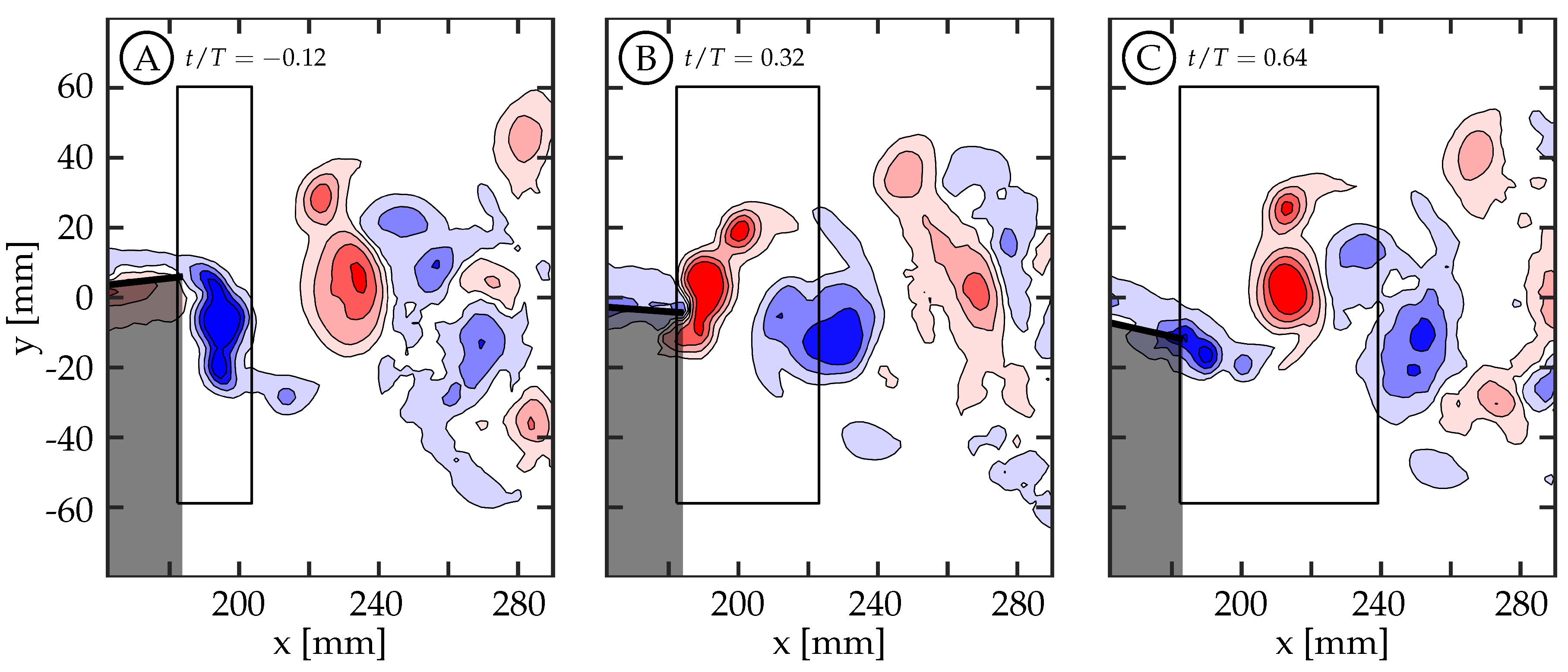
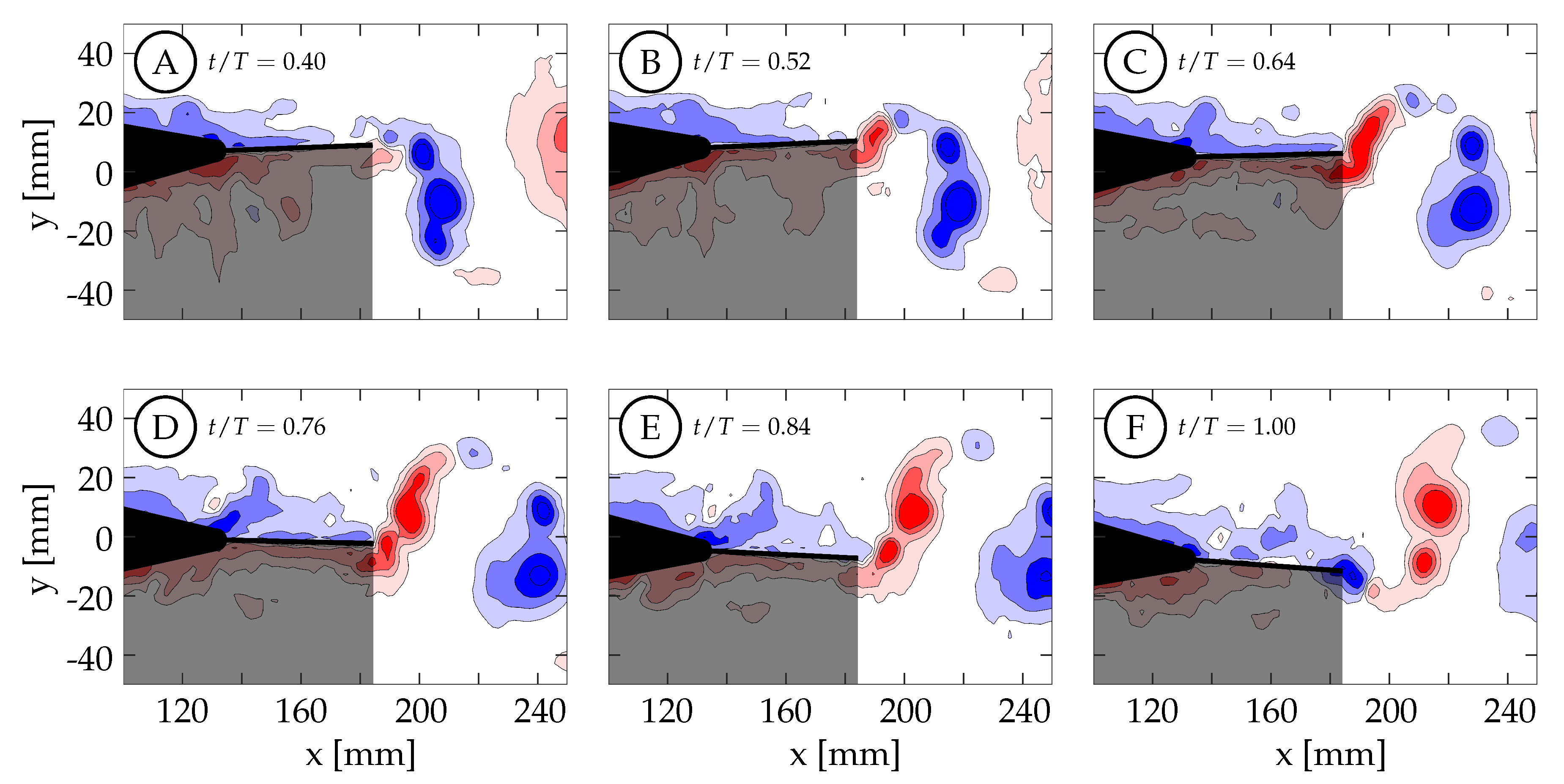
Case 4 is shown in
Figure 16, where
and the kinematics are characterized by a large amplitude tail motion (
) and negligible caudal fin motion (≈
). Phase-averaged TE amplitude and velocity curves versus nondimensional time are shown in
Figure 13D. The kinematic discrepancy is barely apparent in this case due to the negligible caudal fin motion, and therefore this case represents nearly ideal sinusoidal trailing edge motion as is used in many previous studies in the literature. At
(
Figure 16A), the TE is decelerating as it approaches the positive amplitude extreme at the beginning of the second half-cycle (
). The previously generated negative vortices (blue) have been shed while a small amount of positive vorticity (red) has started to form and is already visible at the TE. Between
and
, the TE decelerates until it reaches the positive amplitude extreme at the beginning of the second half-cycle (
Figure 16B). At this time the TE reverses direction and starts to form a strong shear layer. Between
and
, the fin accelerates to its largest downward velocity while the shear layer continues to feed the attached forming vortex (
Figure 16B,C). The velocity is here
out-of-phase with the TE amplitude as expected for an ideal sinusoid and therefore the velocity peak coincides with the TE amplitude zero crossing. At
(yellow circle in
Figure 13D), the vortex is shed and is visible in
Figure 16D. Between
and
, the TE decelerates as it moves downward toward the negative amplitude extreme at the end of the current half-cycle. During this time interval, the shear layer weakens and part of the remaining vorticity rolls up into a secondary vortex that trails the primary vortex (
Figure 16E). At some point before
, the fluid above the fin starts to impinge on its top surface and travel from top to bottom around the TE generating negative vorticity (blue) as seen in (
Figure 16F). From there, similar but opposite kinematics and vorticity arrangement are seen in the next half-cycle.
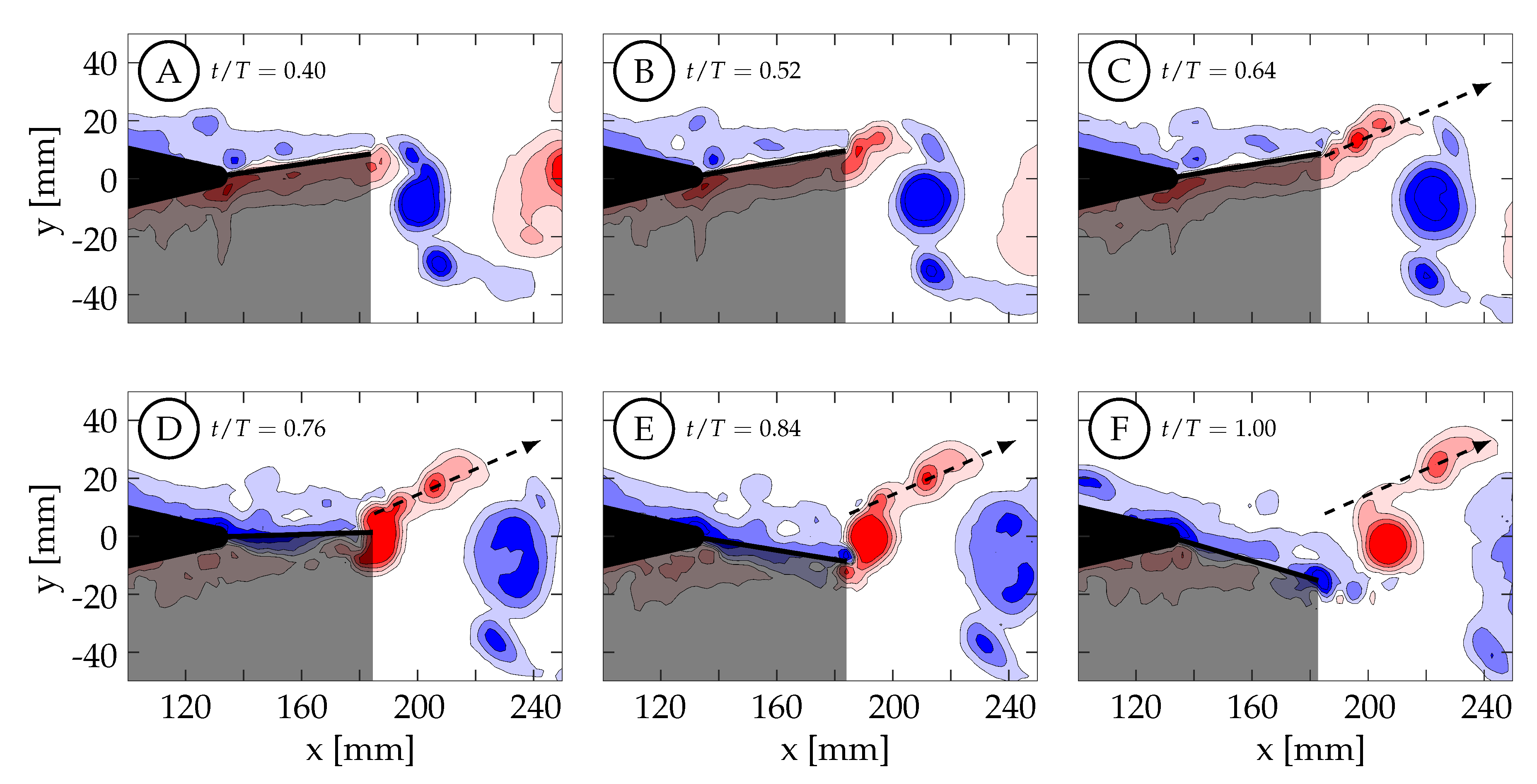
Case 1 is shown in
Figure 15, where
and the kinematics are characterized by a negligible tail motion (≈0.0
) and a large amplitude caudal fin motion (
) that exhibits the discrepancy described in
Section 2.2. Phase-averaged TE amplitude and velocity curves versus nondimensional time are shown in
Figure 13A. At
, the TE is decelerating as it approaches the positive amplitude extreme at the beginning of the second half-cycle (
).
Figure 15A shows that the previously generated negative vortices (blue) have been shed and positive vorticity (red) is visibly being created at the TE as the fin decelerates its upward motion. As in case 4, the fluid below the fin wants to continue moving upward due to its inertia, causing it to impinge on the fin and travel upward around the TE, generating a shear layer. In this case, between
and
the TE decelerates but then remains almost stationary at the positive amplitude extreme due to the kinematic discrepancy. Although the fin is almost stationary, the surrounding fluid continues to move upward due to its inertia. The fluid near the TE continues to travel around the TE, forming a relatively weak shear layer that extends linearly into the wake and can be seen in
Figure 15B,C. As a result of instabilities in the shear layer, it rolls up into several small vortices (
Figure 15C). The largest of these vortices remains coherent and advects downstream following a linear path inclined relative to the
x-direction (see dashed arrows in
Figure 15). Van Buren et al., also observed a small preliminary vortex being formed and shed at the beginning of their square-like profile case [
38]. After
, the TE begins to accelerate as it moves downward, generating a stronger shear layer that rolls up to form an attached vortex. At
, the TE reaches its largest negative velocity at the centerline while continuing to generate vorticity that feeds the attached vortex. The TE then begins to decelerate and the primary vortex is shed at
(yellow circle in
Figure 13A).
Figure 15E shows the primary vortex after it has been shed from the TE. The TE continues to decelerate, weakening the shear layer until at sometime between
and
, the tendency of the fluid on top of the fin to continue downward with its own inertia overcomes the previous flow from bottom to top, and negative vorticity is then generated. The final arrangement of vorticity at the end of the half-cycle is shown in
Figure 15F. At this time (
), the negative amplitude extreme has been reached and the next half-cycle begins. From there, similar but opposite kinematics and vorticity arrangement are seen in the next half-cycle.
The two intermediate cases in this Strouhal number grouping (cases 2 and 3) exhibit similar vortex shedding dynamics. A thorough description is not included here for brevity, but associated figures are included in
Supplementary Figure S1 through S8, which highlight the vorticity generation and organization for all eight cases. As described, in case 1 a shear layer rolls up into a secondary vortex before the trailing edge begins to accelerate and form the primary vortex. In case 4, the panel begins to accelerate sooner, so the shear layer stays attached and forms the primary vortex first. It saturates and sheds, and the trailing shear layer rolls up into secondary structures. In the intermediate cases, the timing of the TE acceleration does move earlier, but the periods of deceleration due to the kinematic discrepancy cause the first vortex to pinch off before saturation, and leaves time for a stronger secondary vortex. As the discrepancy lessens, this effect lessens.
It is deduced that the kinematic discrepancy is not only affecting the magnitude and distribution of vorticity shed from the trailing edge, but likely also the forces generated as well. The time-averaged normalized streamwise velocity for cases 1 through 4 are shown in
Figure 17 while cases 5 through 8 are shown in
Supplementary Figure S9. This quantity is used to visualize regions where momentum has been added to the wake to produce thrust (
, red) and regions of momentum deficit (blue). It is clear that the segmentation of the primary vortex in case 2 (
Figure 17B) cases a bifurcation in the higher velocity jet generated in the wake, and from both the smaller area of momentum surplus, and its relatively lower magnitude, we may assume that a lower force was generated as well. There is also some jet bifurfaction seen in case 1. Cases 3 and 4 exhibit a coherent jet core in the midspan plane, and the magnitude and area is largest in case 4. While we are not able to infer anything specific about the force and efficiency of the fish model, the connections are apparent among body kinematics, trailing edge velocity, vorticity production and organization, and momentum organization.


