Abstract
Wind-waves exhibit variations both in shape and steepness, and their asymmetrical nature is a well-known feature. One of the important characteristics of the sea surface is the front-back asymmetry of wind-wave crests. The wind-wave conditions on the surface of the sea constitute a sea state, which is listed as an essential climate variable by the Global Climate Observing System and is considered a critical factor for structural safety and optimal operations of offshore oil and gas platforms. Methods such as statistical representations of sensor-based wave parameters observations and numerical modeling are used to classify sea states. However, for offshore structures such as oil and gas platforms, these methods induce high capital expenditures (CAPEX) and operating expenses (OPEX), along with extensive computational power and time requirements. To address this issue, in this paper, we propose a novel, low-cost deep learning-based sea state classification model using visual-range sea images. Firstly, a novel visual-range sea state image dataset was designed and developed for this purpose. The dataset consists of 100,800 images covering four sea states. The dataset was then benchmarked on state-of-the-art deep learning image classification models. The highest classification accuracy of 81.8% was yielded by NASNet-Mobile. Secondly, a novel sea state classification model was proposed. The model took design inspiration from GoogLeNet, which was identified as the optimal reference model for sea state classification. Systematic changes in GoogLeNet’s inception block were proposed, which resulted in an 8.5% overall classification accuracy improvement in comparison with NASNet-Mobile and a 7% improvement from the reference model (i.e., GoogLeNet). Additionally, the proposed model took 26% less training time, and its per-image classification time remains competitive.
1. Introduction
The sea is the center of numerous commercial and non-commercial activities, such as maritime transportation, fishing, oil and gas production, and marine and coastal tourism. These activities play a major role in the global economy. For example, the maritime transportation industry facilitates over 80% of global trade by volume [1], the fishing industry has a share of 16% in the global protein production market [2], and the offshore oil and gas sector produces 37% and 28% of the global oil and gas share, respectively [3]. Similarly, marine, and coastal tourism is expected to contribute 26% to the global ocean economy by 2030 [4].
For operational and safety reasons, all activities taking place on the surface of the sea are subject to sea weather conditions. One of the prominent weather phenomena present on the surface of the sea is the wind-wave. These waves are formed by the transfer of energy from wind blowing over large stretches of a water body (i.e., sea surface) [5]. These waves have sharp and forward tilting crests and their asymmetric nature is a well-known feature [6]. The front-back asymmetry of a wind-wave is considered an important characteristic of the sea surface [7]. The sea state, which is the prevailing wind-wave conditions on the surface of the sea [8], is one of the important parameters of the sea weather reporting system and has been listed as an essential climate variable (ECV) by the Global Climate Observing System [9].
It has been reported that offshore oil and gas structures are vulnerable to wind-wave conditions (i.e., sea state), especially the wave height [10]. The contemporary method to measure and classify sea states is through the statistical presentation of wind-wave parameters such as significant wave height (Hs) and average zero-crossing period (Tz) [5]. These parameters are acquired from various traditional sources such as sea buoys, wave radars, and satellite observations [11]. Additionally, numerical wave modeling is used to determine wind-wave conditions [12]. However, due to the (i) high capital expenditures (CAPEX) and operating expenses (OPEX) incurred during the installation, operation, and maintenance of traditional data acquisition sources; (ii) data anomalies originating from sensor malfunctioning or communication breakdown; or (iii) high computational resource and time requirements of numerical modeling, these solutions are costly, especially for offshore oil and gas platforms.
In recent years, deep learning has been widely applied in various fields. For example, in medicine, a method for automatic multi-needle digitization for ultrasound-guided prostate brachytherapy is proposed using large margin mask R-CNN [13]. In astronomy, the detection and classification of various types of galaxies is achieved using a CNN [14]. In the domain of higher education, a CNN-based model facilitates the personalized learning of students by predicting their course grades [15]. For autonomous ship navigation, an improvement of ResNet is proposed to classify maritime navigation markers with high accuracy [16] and small ship detection is performed using a mask-CNN [17]. Similarly, machine and deep learning models have been employed as an alternative solution to forecast and classify wind-wave conditions. A recent survey on the topic has reported superior performance of these new approaches over contemporary numerical wave modeling in terms of efficiency, portability, and lower computational complexity [11]. However, to train and test these models, a large amount of wave parameter data acquired from traditional data sources is still needed. The inherent issues with these traditional data acquisition sources, however, question the cost-effectiveness of these models, especially for offshore oil and gas platforms.
Empirically, sea state can be estimated using The Beaufort wind force scale, which classifies sea state into 13 categories with corresponding wind speeds. The scale provides a concise description of the visual features of each sea state and is adopted by the World Meteorological Organization (WMO) [18]. By identifying these visual features, a sea state can be classified in a maritime scene. This leads to the interesting possibility of classifying a sea state using a deep learning image classification model and a sea image only. Following this approach, in this study, we propose a novel deep learning sea state classification model that classifies the prevailing sea state using visual-range sea image only. The suggested solution requires an optical sensor mounted on an offshore oil and gas platform to capture sea surface images at a regular interval. These images are then classified by the onboard sea state classification model. As a result, the proposed solution not only minimizes the CAPEX and OPEX associated with traditional sea state classification methods but also helps reduce the requirement for a specialized human force for the operational and maintenance purposes of traditional methods.
1.1. Related Work
This subsection presents a review of related work on the topics of sea state datasets and classification using deep learning models. For this purpose, the literature search method described in Appendix A was adopted, and the results presented in Appendix B were referred to.
1.1.1. Sea State Datasets
The global sea state dataset is a novel sea state parameter (i.e., significant wave height and mean wave period) dataset developed from wave model (WM) data acquired from spaceborne advanced synthetic aperture radar (ASAR) measurements [19]. The dataset has a temporal scale of 10 years (i.e., 2002–2012). A data validation approach based on in situ buoy measurements proposed in study [9] was applied to the acquired significant wave height and mean wave period data. The study presented a sea state dataset that has global coverage. The final dataset is presented in NetCDF format, which stores multidimensional numeric data for parameters under observation. The nature of data representation makes this dataset unsuitable for image classification models.
The sea state CC1 dataset v1 was developed using satellite altimeter data collected from ten space missions from 1991 to 2018 [9]. These satellites operated between an altitude of 717 to 1336 km. The collected data was validated using in situ wave parameter observations recorded by moored buoys and fixed platforms in coastal (i.e., <200 km from shore) and deep-sea locations across the globe. A standard for data quality–level was established to accept the measured wave parameters. In its final stage of development, a denoising technique was applied to the data. The final dataset offers a large temporal and geographical range. However, the dataset uses satellite altimetry observations, which makes it unsuitable for image classification models.
Apart from these two prominent datasets, there are studies which have mentioned and used various other sea-related datasets. In one such study by Loizou and Christmas [20], wind speed, period, wavelength, and highest value for significant wave height were estimated from “wave radar image data”. The work presented by Cheng et al. [21] estimated six sea states by applying LSTM, CNN, and a proposed deep learning model using “simulated ship motion data”. A numerical approach to estimate significant wave height presented by Wang and Hong uses horizontally polarized “radar image data” [22]. A very small-scale study conducted by Ampilova et al. [23] distinguished two sea surface conditions by analyzing multifractal spectra of “visual-range sea surface images”. However, the study only discussed two visual-range sea surface images as a test case. Almar et al. [24] suggested an optical geometry-based solution to derive sea surface elevation anomaly from “visual-range images” acquired from drone footage and satellite. The dataset, however, lacks temporal and geographical diversity. Work presented by Rikka et al. [25] proposed an image processing algorithm to estimate significant wave height and wind speed from “synthetic aperture radar (SAR)” satellite data.
In Table 1, a summary of the findings is presented.

Table 1.
Summary of studies reviewed for sea state datasets.
The presented literature review on sea state datasets primarily identified (i) two large-scale sea state datasets [9,19] and (ii) a small scale visual-range sea state dataset [24]. The foremost datasets were presented in undesired formats and used traditional data acquisition sources. However, the visual-range sea state image dataset presented in [24] was found relevant to our study. Upon further investigation, it was observed that the dataset was acquired from an aerial drone, capturing limited temporal and geographical diversity. Furthermore, the dataset was designed to identify sea states using optical geometry. Hence, this dataset was found to be unsuitable for our proposed model. Other datasets, such as ship motion data and radar image datasets, were also identified. However, due to their acquisition methods and data types, they were also categorized as unsuitable for our study.
1.1.2. Sea State Classification Using Deep Learning Models
Deep learning’s application in sea state classification problems is a recent topic of interest. In this context, studies involving various types of sea state datasets and deep learning models are seldom seen [21]. The literature search conducted by the authors resulted in five relevant studies; however, due to access restrictions, one study was not included in this review, the details of which are presented in Appendix B, Table A2. The review of the rest of the studies is presented hereafter.
Tu et al. [27] proposed a feature-based approach employing a three-layer classification model which was trained and tested on four-degree-of-freedom (DoF) ship movement data, namely surge, sway, roll, and yaw. The data was preprocessed to filter out corrupted signals and decomposed into 20 categories for each DoF. For each category, 11 statistical features were extracted, which resulted in 220 features per DoF. For optimal training and testing costs, only the most salient features were identified (i.e., 80) by applying the Max-relevance Min-redundancy (mRMR) method. The first layer of the proposed model was composed of 20 ANFIS classifiers, each associated with every DoF’s category. The sea state classification results of ANFIS were used to train four random forest classifiers (one for each DoF). In the third layer, a bias-compensating weighted averaging method is applied to finally classify sea state from four outputs from RF. The study reported 74.4% to 96.5% sea state classification accuracy (depending on record interval value). Despite its high sea state classification accuracy, it is important to note that the approach used in this study utilized data acquired from ship motion sensors. By relying on numeric data to classify sea states, this study does not address the issue of sea state classification using visual-range sea images.
A novel time-frequency image-based approach proposed by Cheng et al. [28] utilized simulated ship movement data from nine sensors to train and test a convolutional neural networks (CNN). Using short-time Fourier transform (STFT), each sequence of data from the sensors was converted into a single spectrogram. The study bifurcated sea states into 5 categories, and the proposed 2D CNN model was trained to classify the sea states using the spectrogram. The results of 2D CNN were compared to LSTM and CNN trained and tested on 1D ship movement data, and it was identified that LSTM produced the lowest classification accuracy average of 79%. The proposed model, though, resulted in the highest classification accuracy of 94%. However, the study did not report the following: (i) the number of spectrogram instances per class and in the overall dataset; and (ii) the per-class classification accuracy of the proposed model. Thus, the model’s generalization ability across various classes is not known.
Liu et al. [29] proposed sea state classification using LeNet-based model and sea clutter radar data from two sources. The datasets covered three sea states in which significant wave heights ranged from 0.5 m to 4 m. Separate models were trained and tested on the datasets and, subsequently, two classification accuracies, i.e., 95.75% for states 3–4 and 93.96% for states 4–5, were reported. The lower classification accuracy (i.e., 93.96%) was attributed to limited buoy measurement calibration points for corresponding sea clutter radar data (which covers several kilometers). The study claims strong generalization ability. However, the models were tested in a small temporal and geographical setting. Additionally, high class imbalance was observed in the datasets due to which models may exhibit bias towards the majority class [30].
In a study presented by Zhang et al. [31], a ResNet-152 model was used to classify sea states from optical images of the sea surface. The study divided sea states into 10 categories based on ship movement and wave forms. The video data was collected from a ship mounted visual-range video camera. An unusual data split ratio of 82:18 was used to train and validate the model. The model’s validation accuracy was reported to be 89.3%. However, the study does not report any measure to quantify the testing accuracy of the proposed method, nor does it mention sea-state-wise and overall classification accuracy. Additionally, the method, which adopted dividing the sea states into 10 categories, does not follow any recognized standard such as the Beaufort scale [5] or Douglas scale [32]. Thus, the study has little to no significance overall.
In Table 2, a summary of the findings is presented.
Table 2.
Summary of studies reviewed for sea state classification.
1.2. Problem Statement
The sea state is an important parameter of sea weather reporting systems [9] affecting various commercial and non-commercial maritime activities. The conventional methods to classify the sea state are dependent upon sensor or numerical modeling-based acquisition of wave parameters. These methods are thus (i) costly, (ii) prone to sensor malfunctioning and communication errors, and (iii) require high computational cost and time, which, specifically for an offshore commercial installation, is an expensive solution.
Machine and deep learning models have been recently applied to classify sea states from data acquired from sources such as (i) wave radar [29], (ii) actual and simulated ship motion monitoring sensors [27,28], and (iii) visual-range imagery [31]. Furthermore, there are studies that report superior performance of these models over conventional methods [11]. However, these studies either still rely on expensive traditional data sources [11,27,28,29] or their methodology, experiment, and results can be further improved [31].
To fill these gaps, in this paper, we propose a deep learning-based sea state classification model which can classify sea state from visual-range sea image acquired from single optical-sensor mounted on offshore oil and gas platform. However, to train and test such a model, a large-scale visual-range sea state image dataset is publicly unavailable. Hence, the study proposes (i) the development of a novel visual-range sea state image dataset and (ii) a novel deep learning-based sea state classification model using visual-range images. Therefore, the following research questions and corresponding objectives are formulated.
| Research Question 1: | How to design, build, and test a large-scale visual-range sea state image dataset for deep learning-based image classification models? |
| Research Objective 1: | To design and develop a novel large-scale visual-range sea state image dataset suitable for deep learning-based image classification models. |
| Research Question 2: | How to optimally classify sea state from visual-range sea surface images using a deep learning model? |
| Research Objective 2: | To develop and validate a novel deep learning-based sea state classification model that can optimally classify sea states from a visual-range sea image. |
The key contributions and novelties of this study are as follows:
- (a)
- Formulation of comprehensive guidelines for the development of a novel visual-range sea state image dataset.
- (b)
- Development of a novel visual-range sea state image dataset for training and testing purposes of deep learning-based sea state image classification models.
- (c)
- Comprehensive benchmarking of state-of-the-art deep learning classification models on developed sea state image dataset.
- (d)
- Development of a novel deep learning-based sea state image classification model for sea state monitoring at coastal and offshore locations.
The rest of the paper is divided into the following sections: Section 2 discusses the methods and materials adopted to achieve the defined research objectives. The novel visual-range sea state image dataset and its benchmark results are presented in Section 3. In Section 4, the development of the proposed novel deep learning-based sea state image classification model is explained. Later, in Section 5, the proposed model is evaluated, and results are discussed. Finally, Section 6 concludes the study, identifies the limitations, and proposes future work.
2. Materials and Methods
This section describes different methods, operating procedures, and design considerations adopted during the study.
2.1. Novel Visual-Range Sea State Image Dataset Design and Development
For the development of a novel large-scale visual-range sea state image dataset, the authors have previously presented general visual-range sea state image dataset design considerations, field observation recommendations, and experimental guidelines [26]. This section extends the previously presented work.
2.1.1. Ground Truth Reference for the Identification of Sea States in an Image
A ground truth is empirical evidence of true information. The Beaufort wind force scale defines the visual ground truth features of a sea state and corresponding wind speed range [18]. The scale is adopted by the World Meteorological Organization (WMO) and is globally used to describe wind and sea state conditions. This study adopted the wind-induced sea state visual features described in the Beaufort scale as ground truth marking reference in an image. The Beaufort wind force scale for the initial five sea states is presented in Table 3.
Table 3.
The Beaufort wind force scale for the initial five sea states [18].
2.1.2. Sensor Selection, Setup, and Calibration
A standalone or array of high-definition optical sensors, such as a video camera, can be used to capture maritime videos. Further, images at different frame-steps and dimensions can be extracted from these captured videos. The approach is widely used in maritime visual-range image dataset development due to its (i) low cost, (ii) simplicity of setup, and (iii) high image quality [33,34,35]. A similar approach has been adopted for this study. A high-resolution digital single-lens reflex (DSLR) camera (i.e., the Nikon D3400) capable of capturing 24.2 million effective pixels is employed. Throughout the field observation experiments, the sea surface videos are recorded in auto focus mode at 60 frames per second. The frame size of the video is 1920 × 1080 pixels. To capture wave features from different distances and angles, variations in zoom, roll, yaw, and pitch and sensor height from the surface of the sea (i.e., from 2 to 12 m) are applied.
To identify sea state in a maritime scene, in situ measurements of wind speed and visual characteristics of sea surface can be used as reference [18]. To acquire wind speed readings, the study utilized a tripod-mounted weather station (i.e., Vantage Vue by Davis Instruments) which is capable of recording wind speed in a range of 1.7 knots to 173.7 knots. Other weather parameters such as temperature, humidity, atmospheric pressure, and rainfall during experiments are also logged but not fully utilized in this study. The weather data is recorded at a one-minute frequency.
Before each field observation experiment, the following sensor setup and calibration procedures are followed:
- (i)
- The date and inner clocks of the weather station and video camera are synchronized.
- (ii)
- The weather station is setup by entering required parameters, such as unit of measure, longitude and latitude values of the field observation site, estimated weather station height above sea level, and wireless data transmission parameters, etc.
- (iii)
- The weather station is carefully mounted at a location where wind flow is not obstructed by any surrounding object.
- (iv)
- The weather station is operational before video recording is started and data transmission between the weather station and data logger device is verified.
- (v)
- The video camera is either mounted on a tripod or handheld.
- (vi)
- The field of observation is set to either the sea surface or sea plus sky.
- (vii)
- Audio recording is disabled, and the videos are recorded in auto mode and at a maximum resolution of 1920 × 1080 pixels.
2.1.3. Selecting a Field Observation Site
West Malaysia is surrounded by two main water bodies, the Malacca Strait, and the South China Sea. The former is a nearly enclosed body of water, so less water surface area is exposed to the wind. This results in generally calm sea state conditions. The South China Sea is, however, a partially enclosed water body, and thus more dynamic sea state conditions are expected on its surface. To capture all possible sea states across West Malaysia, the study has selected one offshore and four onshore, geographically separated field observation sites facing the Malacca Strait and the South China Sea. Offshore observations (i.e., a maximum of 45 km away from the coastline) are recorded from the bow, starboard, and portside of a cruise ship (call sign 3FNT4). Coastal observations are either made from stable platforms stretching into water bodies or from flat stable surfaces near shore. The field observation sites are highlighted in Figure 1.

Figure 1.
Offshore (red) and onshore (blue) field observation sites across West Malaysia.
2.1.4. Achieving Illumination and Weather Feature Diversity
The sun’s movement across the sky and cloud cover percentage are major factors in varying illumination levels in a maritime scene [34]. Seasonal wind speed and direction variations are the sources of changing sea state levels. For example, the monsoon season has been reported to influence sea conditions [35].
For better generalization ability of the DL classification model, it is important that such features are represented in the visual-range sea state image dataset. Thus, to capture features observed across the day and at different seasons, the field data collection experiments were conducted on 10 different occasions (from February 2020 to April 2021). These occasions were selected based on sought-after illumination, weather, wind, and sea state conditions at observation sites. For example, sea state images were captured at different times of the day and cover the illumination levels of the late morning, noon, afternoon, evening, and late evening conditions. As a result, various sea surface illumination, glare, and glint levels due to the sun’s movement across the sky are captured in the images. Additionally, the study was conducted under sunny, partly cloudy, overcast, and drizzle conditions during the summer and monsoon seasons. This results in capturing different sea surface colors due to sky conditions, textures due to drizzle, and wave conditions due to monsoon season.
2.1.5. Defining Optimal Range of Image Instances per Class for the Dataset
For an image classification problem, it is generally a good approach to use a large amount of data for model training, validation, and testing. As the literature suggests, the minimum number of instances per class on which a DL classification model can be trained and tested successfully is approximately 1000 [36]. Similarly, a popular image classification dataset, ImgeNet [37], aimed at 500 to 1000 images per synset. So, 1000 or more image instances are sufficient to optimally train and test a deep learning image classification model. Thus, for our proposed dataset, it is deduced that image instances between 1000 and 5000 per class is an optimal range.
2.2. Data Collection and Preprocessing
2.2.1. Wind and Video Data Collection and Preprocessing
For sea state estimation, wind is the relevant weather parameter to use. During the field experiments, a weather station is used to record wind and other weather parameters on external storage at a one-minute frequency. In this study, a half-hourly average of wind speed (in knots) is calculated and used as a ground truth reference to estimate sea state.
The sea surface videos are captured from various heights (2–12 m above sea level) and with varying zoom, roll, yaw, and pitch levels. Videos are shot at various lengths (i.e., from a few seconds to 15 min) and at different times of the day to capture changing illumination levels. During all video capture experiments, the camera was set to autofocus mode. Approximately 8 h of footage (i.e., 162 video files, 1.7 million frames) of sea videos was recorded. All 162 video files were manually evaluated for optimal sea surface image extraction. At this stage, 135 videos were selected for sea surface feature extractions. An example of this manual selection process is presented in Figure 2.
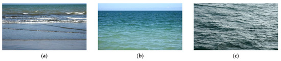
Figure 2.
Video selection process for sea surface feature extraction: (a) rejected video: sea surface features are not dominant in the frame; (b) accepted video: sea surface features are dominant and can be cropped from the video frame; (c) accepted video: full exposure to the sea surface features.
2.2.2. Sea State Estimation in Video
As described previously, the study referred to the Beaufort wind force scale to establish ground truth for sea state estimation. The Beaufort wind force scale defines the visual characteristics of different sea states and their corresponding wind speed ranges. A matrix is thus formed to manually classify the videos into various sea states. The classification matrix with one video classification example is described in Table 4.
Table 4.
Sea state manual classification matrix.
Each video is evaluated on the abovementioned matrix. First, wind speed recorded at the time of video capture and corresponding half-hourly wind speed in knots are analyzed and sea state is marked. The wind speed ranges defined in Table 5 are used to mark a sea state.
Table 5.
Wind speed range and corresponding sea state.
The second approach to classifying the same video is based on visual inspection of sea surface features in the video and their similarity to features defined by the Beaufort wind force scale [18,38]. The complete length of the video is manually analyzed, and the sea state is identified only if all the corresponding visual features are present in the video.
At this stage, a video is excluded from the study if its wind-based sea state classification does not match with its visual attributes-based classification. As a result, a total of 83 videos were finally classified into five sea states, ranging from 0 to 4.
2.2.3. Image Extraction from Video Source
The videos recorded in this experiment have 1920 × 1080-pixel dimensions. Due to geographical diversity and various sea-to-sky ratios in maritime scenes captured in the videos, a universal image extraction approach based on fixed image dimensions results in the presence of unnecessary background or foreground objects in the image. Thus, in such videos, images are extracted at video-specific optimal image extraction dimensions. Videos having full exposure to the sea surface features are fully utilized and, from one video frame, two images are extracted at a fixed 1280 × 720-pixel dimension, having a 20% vertical overlap. Additionally, images are extracted at different suitable frame intervals. As a result, only images depicting the sea surface are extracted to the greatest extent possible.
2.2.4. Handling Class Imbalance and Defining Dataset Splits
Class imbalance is an inherent issue in real-world scenarios. An imbalanced dataset may cause a model’s bias towards the majority class and, in some cases, complete ignorance of the minority class [30]. To address this issue, the following steps are followed:
- The fixed maximum number of image instances per class is defined as N.
- Videos in each class are manually split into disjointed training, validation, and testing sets.
- From each video in a disjointed set, a set-specific fixed number of instances are randomly selected to populate raw training, validation, and testing image pools.
- A few exceptions are made when certain videos in a set have a lower number of instances than the set-specific fixed number. In this case, all instances from such videos are selected.
- From each class’s training, validation, and testing pool, image instances are randomly selected such that they are equal to N and follow a 60:20:20 ratio.
2.2.5. Data Augmentation
Data augmentation is a technique to increase the quantity and quality of a dataset [39]. Additionally, to improve the generalization ability of deep learning-based image classification models, data augmentation can be applied to training and validation sets [38]. A similar approach is adopted in this study, and data augmentation is applied to both the training and validation sets.
Data augmentation methods, such as geometric transformation, kernel filters, mixing images, random erasing, and transforms [39], are evaluated for their suitability for maritime scene (i.e., sea state image) augmentation. The details of this evaluation are given in Table 6.
Table 6.
Suitability analysis of data augmentation methods for sea state images.
The selected augmentation methods are applied to build an image augmentation pipeline (IAP) for sea state images. Each image from the training and validation set of each class is first resized to 224 × 224 pixels before augmentation. The flow of IAP is illustrated in Figure 3.
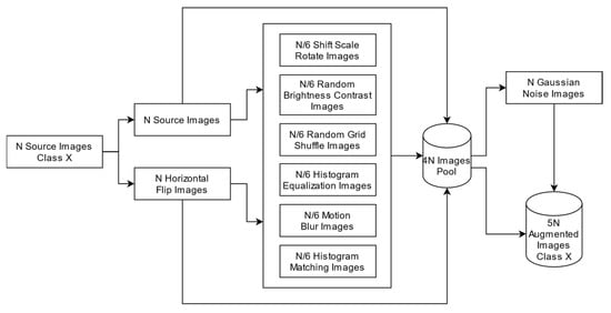
Figure 3.
Image augmentation pipeline (IAP) for sea state classification.
2.2.6. Image Naming Conventions
To keep track of the source video files, frame sequence number of the extracted image, image size, and applied augmentation sequence etc., an image naming conventions is formulated and presented in Table 7.
Table 7.
Image naming convention.
An image named “DSC_0127_FA_900_224×224_HF_RBC_GN” thus indicates that the image’s source video is DSC_0127. It is the first overlapping image from frame 900, which is resized to 224 × 224 pixels with a horizontal flip, random brightness and contrast, and Gaussian noise applied to it.
2.3. Hardware and Software Environments
Various data preprocessing, deep learning model training, and testing experiments are performed in the study. The hardware and software environments presented in Table 8 are used in those experiments.
Table 8.
Hardware and software environments.
3. Visual-Range Sea State Image Dataset
3.1. Dataset Development
3.1.1. Narrowing of Sea State Classes
Following the methodology presented in the previous section, ten field observation experiments were conducted across West Malaysia. The data preprocessing resulted in the identification of five sea states in the acquired data, a summary of which is presented in Table 9.
Table 9.
Preprocessed sea state video data summary.
At this stage, sea state 0 is excluded from the study due to its extremely limited presence (i.e., two videos) in the raw data. This limitation eventually resulted in similar environmental and weather features in all extracted images for sea state 0.
3.1.2. The Final Dataset
Two observations played pivotal roles in the development of the proposed dataset: (i) training of a deep learning classification model requires a large, labeled dataset; and (ii) variations in image dynamics can enhance the model’s generalization ability.
The first observation was incorporated by initially selecting 6000 source images per class. These images were split into disjointed training, validation, and testing sets. By applying label preserving augmentation techniques on training and validation sets, the overall instances of images in a class were extended to 25,200. Since the dataset represents 4 sea states (i.e., 1 to 4), in its final form, the dataset offers 100,800 images.
To incorporate the second observation, the development methodology of the dataset enforced acquisition of the maximum range of sea-state dynamics observed during field data collection experiments, namely daily illumination, glint, and glare variations; sensor induced features (i.e., zoom, pitch, roll, sensor height); weather variation (i.e., clear sky, cloud cover, drizzle); seasonal variations (i.e., monsoon, summer); and sea surface color.
In its final form, we name this dataset Manzoor-Umair: Sea State Image Dataset (MU-SSiD). Detailed statistics of MU-SSiD are presented in Table 10 and Table 11 and representative image instances are presented in Figure 4.
Table 10.
Statistics for MU-SSiD source image sets.
Table 11.
Statistics of final MU-SSiD.
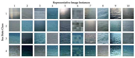
Figure 4.
MU-SSiD per-class representative image instances.
3.2. MU-SSiD Classification Accuracy Benchmark Experiments
To evaluate the usefulness of MU-SSiD and to establish a benchmark classification accuracy matrix for MU-SSiD, the classification performance of 19 pretrained state-of-the-art deep learning image classification models was examined using MU-SSiD. For the interest of the reader, brief descriptions of these models are presented hereafter.
3.2.1. AlexNet
AlexNet is the winner of ILSVRC-2012 and achieved a 15.3% top-5 test error rate on the subset of ImageNet dataset [36]. The model applied a dropout technique to reduce overfitting and GPU based implementation of convolution operations. At the time of its publication, AlexNet was the largest convolution neural network.
3.2.2. VGG Family (VGG-16, VGG-19)
The VGG models are the winner and runner-up of ImageNet Challenge 2014 for localization and classification [41]. The models effectively used the smallest possible filter sizes with very deep convolutional networks (16 and 19 weight layers), resulting in top-5 test error rate of 6.8% and 25.3% in the ILSVRS classification and localization tracks, respectively.
3.2.3. Inception Family (GoogLeNet, Inception-v3, Inception-ResNet-V2)
The inception deep learning model family, particularly GoogLeNet, is based on multiple repetitions of an inception module. The inception module is based on the network-in-network approach and attempts to optimally approximate the local sparse structure of the convolutional vision network. The model GoogLeNet is the winner of the ILSVRC 2014 competition and resulted in 6.67% top-5 error accuracy [42]. Inception v 1-4 and Inception-ResNet are different versions of GoogLeNet that are publicly available
3.2.4. ResNet Family (ResNet-18; ResNet-50; ResNet-101)
The basic ResNet is inspired by the VGG nets, and it addresses the degradation problem associated with deep neural networks [43]. The term “degradation” refers to a decrease in the network’s performance on test and training data as its depth is increased. The ResNet model employs a shortcut connection for identity mapping, the output of which is added to the output of the stacked layer. This makes it possible to develop and train a deeper network without being concerned about degradation problems. As a result, a much deeper ResNet (i.e., 8× deeper than VGG nets) resulted in lower complexity, easy optimization, and, compared to the state-of-the-art models, its ensemble yielded an improved top-5 error rate of 3.57%. The ResNet is also the winner of the ILSVRC 2015 competition.
3.2.5. SqueezeNet
SqueezeNet is a small convolutional neural network which is designed for distributed training, lower bandwidth needs for “cloud to autonomous vehicle model” export, and devices with limited memory. SqueezeNet has 50× fewer parameters compared to AlexNet and yielded equal classification accuracy on ImageNet.
3.2.6. MobileNet-v2
MobileNet is a lightweight deep neural network developed for mobile and embedded vision applications. Its architecture is based on depth-wise separable convolutions. With the use of global hyper-parameters, the model facilitates selection of the right-sized model based on the nature of the problem. The model resulted in better classification accuracy compared to GoogLeNet, SqueezeNet, and AlexNet [44].
3.2.7. Xception
The Xception model is inspired by inception architecture [45]. The model substituted the inception module with depthwise separable convolutions and has residual connections. On a large dataset containing 350 million instances across 17,000 classes, Xception outperformed Inception-v3 and other state-of-the-art models by yielding 0.79 and 0.945 top-1 and top-5 accuracy, respectively.
3.2.8. Darknet Family (DarkNet-19; DarkNet-53)
The Darknet model [46] is the basis of YOLOv2, which is a real-time, state-of-the-art object detection system. The design of Darknet is inspired by the VGG models and network-in-network. To process an image, the model only performs 5.58 billion operations and yields 72.9% top-1 accuracy and 91.2% top-5 accuracy on ImageNet.
3.2.9. DenseNet-201
The design of DenseNet is based on the idea of introducing shorter connections between layers near to input and output. Each layer of DenseNet is connected to its succeeding layers’ output. In this fashion, a DenseNet with L layers has direct connections. Because there is no need to relearn redundant feature maps with dense connections, fewer parameters are required as compared to typical convolutional neural networks. The model achieved 3.46% error rate on the augmented CIFAR dataset, surpassing the performance of state-of-the-art models such as ResNet [47].
3.2.10. NASNet Family (NASNet-Mobile; NASNetlarge)
The NASNet model is based on stacked convolution layers, which improves its generalization ability using a novel regularization technique called ScheduledDropPath. During training, this regularization technique drops out each path in the convolutional layer based on linearly increased probability. The model resulted in a reduction of 28% in computational demand and a 3.1% top-1 accuracy improvement as compared to state-of-the-art models [48].
3.2.11. ShuffleNet
ShuffleNet is an efficient convolutional neural network designed for low computational power mobile devices. To reduce computational cost, the model uses pointwise group convolution and channel shuffle operations. ShuffleNet achieved a 13× speedup over AlexNet and exhibited a 7.8% top-1 error as compared to MobileNet [49].
3.2.12. EfficientNet-b0
The EfficientNet family [50] of convolutional neural networks was developed using a model scaling method which addresses balanced network depth, width, and resolution growth based on a novel compound scaling method. The method uses a compound coefficient that controls the available resources for scaling. As a result, it produced an 84.3% top-1 accuracy on ImageNet. Additionally, its transfer-learning ability also remains competitive for various datasets.
A summary of these pretrained models and their training parameters are listed in Table 12 and Table 13 respectively.
Table 12.
Pretrained deep learning image classification model summary.
Table 13.
Model training parameters.
3.3. Benchmark Classification Accuracy Experiment Results and Discussion
The proposed dataset (i.e., MU-SSiD) was evaluated for its suitability for sea state classification problem. The dataset was tested using state-of-the-art deep learning classification models which were trained and tested on the hardware and software configurations presented in Section 2.3.
During the model training experiments, two models, i.e., Inception-ResNet-V2 and nasnetlarge, failed to train due to GPU memory constraints. Additionally, three models’, i.e., AlexNet, VGG-16, and VGG-19, validation accuracies were recorded to be the lowest (i.e., 25%). Thus, these untrained and underperforming five models were excluded from the testing experiments.
The remaining 14 models were tested on the test set of MU-SSiD. The highest classification accuracy of 81.8% was produced by NASNet-Mobile. The model, however, recoded the highest per-image classification time of 0.127 s. The lowest per-image classification time of 0.012 s was achieved by SqueezeNet, which, however, performed poorly for the classification task (i.e., 41.9% classification accuracy).
For class-wise classification accuracy, the highest classification accuracy was recorded for sea state 4 (i.e., 100%). The results remain the same except for SqueezeNet and DarkNet-19. A possible explanation for this can be traced back to the fact that the image instances presented in the dataset for sea state 4 are limited to only five videos. These instances have little environmental diversity and present no seasonal diversity. Thus, similar image features are present both in the training and testing splits. Even though multiple augmentations have been applied to the training set, the issue pertains. This observation highlights one limitation of MU-SSiD.
The second highest class-wise classification accuracy of 97.0% was recorded for sea state 1 by ResNet-101 and across all 14 models, the average class 1 classification accuracy was observed at 82.6%. Sea state 2 was classified with a maximum accuracy of 85.5% by SqueezeNet, and the average classification accuracy for the class was 67.1%. Finally, sea state 3 was best classified by ResNet-101. However, in comparison to the other three sea states, the classification accuracy of sea state 3 remains the lowest, i.e., 65.5%. This can be attributed to feature similarities between adjacent sea states (i.e., state 2 and 3), which makes it difficult for pretrained models to optimally classify sea state 3. In Table 14, detailed classification results for all 14 models are presented for the reader’s interest.
Table 14.
Benchmark sea state classification results.
A comparative graph of model parameters and corresponding overall classification accuracy reveals that the top performing model has the least number of model parameters (i.e., 5.3 million). Additionally, among the top five performing models, three models have equal to or less than 7 million parameters (highlighted by the red rounded rectangle in Figure 5). This may indicate that “higher sea state classification accuracy can be obtained by using smaller and less dense models.” In Figure 5, the comparative graph is presented.
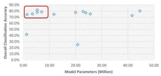
Figure 5.
Model parameters and corresponding overall sea state classification accuracy.
4. Proposed Sea State Classification Model
4.1. Optimal Classification Model Identification
A standard practice in the development of deep learning models is to avoid reinventing the wheel by choosing an optimal reference model from previously proposed models. That model is usually taken as a starting point to develop a new, improved model. One such example is GoogLeNet, which took inspiration from the network-in-network approach [42]. Following the norm, to identify an optimal reference model, the top five models from the MU-SSiD performance benchmark results were evaluated against factors such as (i) simplicity of the model, (ii) lower training time, (iii) higher classification accuracy, and (iv) lower image classification time. The identified optimal values are highlighted in Table 15, which identifies GoogLeNet as an optimal model, excelling in most evaluation factors.
Table 15.
Top five models’ analysis of optimal model identification.
4.2. Climbing the Pinnacle of Classification Accuracy for GoogLeNet
GoogLeNet uses a network-in-network approach. Its fundamental building block is an inception layer which is repeated many times to develop the final model. The model has a depth of 22 and has 144 layers. We propose building a novel sea state classification model on a similar architecture. For this purpose, we first examined our hypothesis that “a smaller and less dense network is most likely an optimal design consideration to achieve high sea state classification accuracy.” To test his hypothesis, a modular approach was adopted to determine the effect of increasing inception blocks on sea state classification accuracy. Models based on one, two, and three stacked inception blocks (1-IB, 2-IB, and 3-IB) of pretrained GoogLeNet were trained and tested on MU-SSiD. The architectures of these three models are depicted in Figure 6.
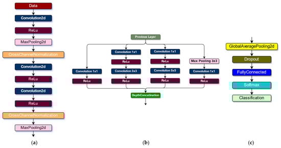

Figure 6.
Evaluated variations of GoogLeNet: (a) initial layers, (b) inception block, (c) final layers, (d) 1-IB Model, (e) 2-IB Model, (f) 3-IB Model.
During this experiment, the initial learning rate and L2 Regularization values were also tuned and set to 0.001 and 0.01 respectively. The rest of the training parameters remain the same as in Table 15. The testing results indicated that the classification accuracy decreased with the addition of the third inception block. The highest classification accuracy (i.e., 85.4%) was observed with two inception blocks, which also surpassed the highest classification accuracy (81.8%) yielded by NASNet-Mobile in performance benchmarking experiments. Table 16 and Figure 7 show the detailed results of the tests performed on these three models.
Table 16.
Results of experiments with increasing inception blocks.
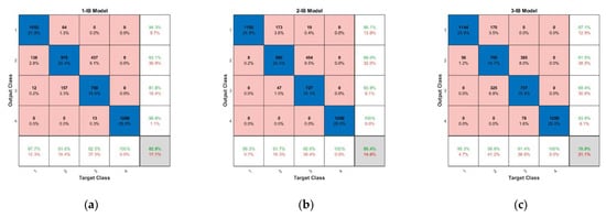
Figure 7.
Confusion matrices for (a)1-IB, (b) 2-IB, and (c) 3-IB models.
These experiments identified the effect of the model’s depth on classification accuracy and validated that a smaller and less dense network is an optimal design approach to achieve high sea state classification accuracy.
4.3. Proposed Model Development
The design idea of our proposed model is inspired by GoogLeNet, which consists of 9 inception blocks. Based on the results presented in Table 16, it is evident that for sea state classification problems, deeper models are not the optimal model design direction and satisfactory classification accuracy can be achieved using a simpler model architecture. For our proposed model, we took a bottom-up approach and chose the 1-IB variation of GoogLeNet as the development starting point and propose gradual performance improvements in the inception block. The general architecture of the proposed model is presented in Figure 8.
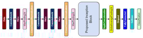
Figure 8.
Architecture of proposed sea state classification model.
It is important to note that each proposed improvement in the inception block is incorporated into its predecessor. We proposed changes in (i) filter parameters to extract a higher number of abstractions and to capture various levels of contextual information from dynamic sea surface images; (ii) the increase in inception block width as one proven approach to improve the performance of deep neural networks; and (iii) the addition of a dropdown layer to minimize overfitting.
4.3.1. Design Improvement 1—Filter Parameters
The original first inception block of GoogLeNet has various combinations of numbers of filters and sizes suitable for object classification. For sea state classification, we first proposed to change the number of filters in inception block. The proposed number of filters start from 16 and is increased by a power of 2. Upon filter parameter updates, the inception block is presented in Figure 9.

Figure 9.
Inception block with filter number modification.
4.3.2. Design Improvement 2—Increasing Width of Inception Block
The second design change in inception model is proposed in its width [42]. We introduced additional 3 × 3 convolution layer and lowered the filter number range from 16 to 8. After proposed amendments, the inception block’s architecture is as presented in Figure 10.
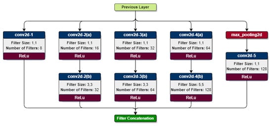
Figure 10.
Inception block width increment with filter number modification.
4.3.3. Design Improvement 3—Retrieving Contextual Information
The third design improvement introduced one more vertical layer into inception block. The added convolution has higher number of filters and increased filter size (i.e., 7 × 7). This design was inspired by the fact that the features of sea states are local as well as global (i.e., the wave forms and white caps), and thus bigger filter size is necessary to capture the contextual information for sea waves. The proposed design changes are presented in Figure 11.
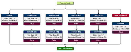
Figure 11.
Addition of second convolution layer with higher filter numbers and size.
4.3.4. Design Improvement 4—Minimizing Overfitting
Dropout is a simple and easily implementable powerful regularization technique to minimize overfitting in deep learning models [51]. To handle overfitting, we introduced dropout layers in our fourth design improvement. These dropout layers are added into inception block. The updated block architecture is depicted in Figure 12.
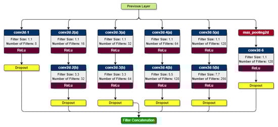
Figure 12.
Addition of dropout layers.
5. Proposed Models Evaluation and Discussion
The benchmark performance experiment identified NASNet-Mobile as the top model in terms of classification accuracy (i.e., 81.1%). In a comparative analysis presented in Table 15, GoogLeNet was identified as the most optimal model for sea state classification. The results presented in Figure 5 indicate that a less dense deep learning model can also yield higher sea state classification accuracy. These facts motivated us to explore and experiment with less dense versions of GoogLeNet. These models, namely 1-IB, 2-IB, and 3-IB, were tuned and an optimal initial learning rate and L2 regularization values were identified. This resulted in the highest classification accuracy of 85.4% for the 2-IB Model. To further improve the classification accuracy, four systematic and gradual design improvements in the inception block were proposed. Following a bottom-up approach, these changes were proposed in the original pretrained GoogLeNet model with one inception block (1-IB). This model took 12 min to train on MU-SSiD and produced an overall classification accuracy of 82.9%.
The first design improvement removed weights from the first inception block of GoogLeNet and updated the number of filters in convolution layers following an increasing order of the power of 2. This modified inception block replaced the original inception block as per the scheme depicted in Figure 8. The resultant model is referred to as Model-1, which was then trained and tested on MU-SSiD. As compared to results produced by 1-IB, Model-1 took 65% more time to train and yielded a 4% decrease in overall classification accuracy while maintaining a similar per-image classification time (i.e., 0.008 s). When compared with 1-IB, a drastic decrease in classification accuracy for sea states 1 and 3 was observed. Additionally, the precision values for 1, 2, and 4 classes also took a dip, except for class 3, which increased from 81.6% to 100%. In Figure 13, the confusion matrix of Model-1 is presented.

Figure 13.
Model-1 confusion matrix.
Our second design increased the width of the inception block by adding one vertical layer along with updated filter numbers and size. This block, when placed in the scheme presented in Figure 8, creates Model-2. In comparison with 1-IB, the model utilizes 39% less training time with a slight improvement in classification accuracy in comparison with Model-1. There was no significant change in per-image testing time with respect to the reference model (i.e., 1-IB). When compared to its predecessor, the current model generally exhibited an improvement in precision values. Similarly, for classes 1 and 2, the classification accuracy of the model also improved. However, this model failed to match Model-1’s classification performance for class 3. The confusion matrix of Model-2 is presented in Figure 14.

Figure 14.
Model-2 confusion matrix.
Our third design adds one more vertical layer with an increased filter number, and especially the filter size, since it has been observed that sea state 3 is mostly classified as sea state 2 by evaluated models. This may be due to the designs of models, which focus more on identifying local features in an image by using smaller filter sizes. In the case of a sea surface image, the similarity between wave forms across two adjacent sea states warrants that feature being extracted on a global scale to distinguish one sea state from another. To test this assumption, the filter size was increased. As per the design presented in Figure 8, this change constitutes our Model-3. By analyzing its training and testing results, it was found that adding vertical layer with increased filter numbers and size resulted in relatively little increase in overall classification accuracy (1%) and a decrease in training time (8%) when compared to 1-IB. The proposed model’s per-image classification time also remained competitive at 0.011 s. Model-3 produced an overall classification accuracy of 83.4%, which is an improvement over NASNet-Mobile (i.e., 81.8%) and 1-IB (i.e., 82.9%). Additionally, the proposed changes resulted in improved classification accuracy of sea state 3 as compared to Model-1 and Model-2. The classification results of Model-3 are presented in Figure 15.

Figure 15.
Model-3 confusion matrix.
The fourth and final design introduced dropout layers in the inception block. The aim was to minimize overfitting. This design formulated the Model-4, which when trained on MU-SSiD reduced the training time by 26% in comparison to 1-IB, and significantly increased overall classification accuracy to 88.7%, which is an 8.5%, 7%, and 4% overall classification accuracy improvement over the NASNet-Mobile, 1-IB, and 2-IB models, respectively. The model also showed superior and competitive precision values against all four classes. On the other hand, for class three, classification accuracy was also improved from 45.9% to 63.4% (within proposed models). Based on its superior classification performance, low training and testing time, we therefore propose Model-4 as our novel sea state image classification model and name it Manzoor-Umair Sea Net (MUSeNet). In Figure 16, the confusion matrix for MUSeNet is presented.
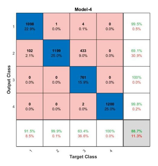
Figure 16.
Model-4 (MUSeNet) confusion matrix.
In Table 17, classification accuracies for all four proposed models are presented. Additionally, in Table 18, an overall performance summary of models is presented, which covers the model’s overall classification accuracy, 95% confidence interval (computed for binomial proportion, which is defined as the number of successes divided by the number of trials), and per-image classification time.
Table 17.
Classification accuracies of proposed models.
Table 18.
Overall comparative performance summary of models.
These experimental results show that (i) the proposed visual-range sea state image dataset, MU-SSiD, can be utilized for sea state classification problems using deep learning models; and (ii) the proposed sea state classification model (MUSeNet) surpassed state-of-the-art deep learning image classification models by yielding 88.7% overall classification accuracy, 26% less training time, and competitive per-image classification time. The total model parameters of MUSeNet are 2 million, which is significantly less than the top performing model identified in the baseline performance experiment (i.e., NASNet-Mobile—5.3 million parameters). The study also signifies the effects of filter numbers, filter size, model width increment, and dropout layer for classification of sea state from visual-range images.
6. Conclusions and Future Directions
Wind waves are generally present on the sea surface. These waves are asymmetric in nature, and their front-back asymmetry is considered an important characteristic of the sea surface. The prevailing conditions of wind-waves constitute a sea state, which is an important parameter for describing sea weather and an essential climate variable of the Global Climate Observing System. Contemporary methods to classify sea states are based on statistical representation of wave parameters or by numerical modeling. These methods are costly, prone to equipment malfunction, and require high computation power and time. As an alternative, image classification can be applied to classify sea states from visual-range sea images. Firstly, in this study, we proposed a novel visual-range sea state image dataset (MU-SSiD) to train and test deep learning sea state classification models. In its final form, MU-SSiD has 100,800 sea state images under four sea state classes (1 to 4 on the Beaufort scale). The dataset was benchmarked against state-of-the-art pretrained deep learning image classification models. Secondly, a novel sea state classification model named MUSeNet was proposed. The model was inspired by the GoogLeNet inception block design. Multiple systematic design changes in filter numbers and size, network width, and layers were proposed in the inception block. As a result, the proposed model yielded a superior overall sea state classification accuracy of 88.7% (i.e., a 7% classification accuracy gain from the top performing model) and 26% less training time.
Two limitations of the study were observed. First, the limited instances for classes 0 and 4 were noted during the dataset creation process, which resulted in the drop of sea state 0 data from the study. The data for sea state 4 was, however, used to develop the dataset for its relatively higher instances. However, high feature similarities were observed in sea state 4’s training, validation, and testing sets. This resulted in 100% classification accuracy for sea state 4 in almost all evaluated models. Second, despite the fact that the proposed model MUSeNet exhibited very high class-wise classification accuracies for classes 1, 2, and 4 (i.e., 91.5%, 99.9%, and 100%, respectively), the classification accuracy for class 3 remains low, at approximately 64%. This affected the overall classification accuracy of MUSeNet. The results showed that the proposed model did not distinguish well between adjacent sea state classes (i.e., 2 and 3).
As a future work for MU-SSiD, we propose the addition of sea state 0 instances and feature diversity in sea state 4 instances. Additionally, for MUSeNet, design changes that improve the accuracy of classification for sea state 3 can be looked into.
Author Contributions
Conceptualization, M.A.H., M.U., H.T. and M.N.A.; methodology, M.U. and M.A.H.; software, M.U.; validation, M.U., S.S.H.R. and M.M.M.; formal analysis, M.U.; investigation, M.U., S.S.H.R. and M.A.H.; resources, M.A.H.; data curation, M.U.; writing—original draft preparation, M.U. and M.A.H.; writing—review and editing, M.U., M.A.H., H.T. and M.N.A.; visualization, M.U.; supervision, M.A.H.; project administration, M.A.H. and M.U.; funding acquisition, M.A.H. All authors have read and agreed to the published version of the manuscript.
Funding
This research was funded by Yayasan Universiti Teknologi PETRONAS—Fundamental Research Grant (YUTP-FRG-2019, grant number 015LC0-158).
Institutional Review Board Statement
Not applicable.
Informed Consent Statement
Not applicable.
Data Availability Statement
The Manzoor Umair: Sea State Image Dataset (MU-SSiD) can be downloaded from https://www.kaggle.com/datasets/umairatwork/mu-ssid (accessed on 16/07/22).
Acknowledgments
The authors would like to thank Syed Muslim Jameel for his support in local transportation of equipment and materials.
Conflicts of Interest
The authors declare no conflict of interest.
Appendix A. Literature Search Method
An image classification model requires a comprehensive subject-specific image dataset for training, validation, and testing purposes. Thus, as a first step, there is a need to identify publicly available sea state datasets and evaluate their suitability for the proposed model. Secondly, before proceeding to the development of the proposed sea state classification model, current research in the field of deep learning-based sea state classification must be identified and reviewed. Appendix A describes the literature search method adopted to identify relevant literature.
The following steps are defined to formulate a literature search method.
- Domain-specific keywords are chosen and based on their combinations, six search queries are generated.
- The queries are executed on three search engines, i.e., (i) Web of Science, (ii) Scopus, and (iii) Google Scholar.
- For each query, studies conducted in English from 2018 till 2022 are filtered.
- The titles of the first 25 studies (sorted by relevance) are reviewed and relevant studies are shortlisted.
- The abstracts of shortlisted studies (whose full manuscripts are available) are reviewed, and the most relevant studies are selected for literature review.
The information on domain, corresponding keywords, assembled queries, and search engines used to identify relevant literature published in the previous 5 years is provided in Table A1.
Table A1.
Literature search parameters.
Table A1.
Literature search parameters.
| Domain | Keywords | Queries | Search Engines |
|---|---|---|---|
| Dataset | Sea state, Image, Dataset | Sea state, Sea state image, Sea state dataset, Sea state image dataset | Web of Science, Scopus, Google Scholar |
| Classification | Sea state, Image, Classification | Sea state classification, Sea state image classification |
Appendix B. Literature Search Results
By analyzing the titles retrieved from search queries, 26 unique articles were shortlisted. The abstracts of accessible shortlisted studies were reviewed. Two flags, Direct and Indirect, were used to identify the relevance of a study. A study was flagged as Direct if it addresses the topic directly. An Indirect flag indicates that the study addresses the topic in an indirect fashion and useful information may be retrieved. Finally, 13 studies (9 for the dataset and 4 for classification) were selected for the final literature review. Table A2 presents the results of the literature search.
Table A2.
Literature search results.
Table A2.
Literature search results.
| SN | Research Domain | Study Title | Relevance | Document Available | Final Status |
|---|---|---|---|---|---|
| S1 | Dataset | Observing sea states | No | - | Excluded |
| S2 | Dataset | A global sea state dataset from spaceborne synthetic aperture radar wave mode data | Direct | Yes | Included |
| S3 | Dataset | A large-scale under-sea dataset for marine observation | No | - | Excluded |
| S4 | Dataset | Deep-sea visual dataset of the South China sea | No | - | Excluded |
| S5 | Dataset | East China Sea coastline dataset (1990–2015) | No | - | Excluded |
| S6 | Dataset | Estimating pixel to metre scale and sea state from remote observations of the ocean surface | Indirect | Yes | Included |
| S7 | Dataset | Heterogeneous integrated dataset for maritime intelligence, surveillance, and reconnaissance | No | - | Excluded |
| S8 | Dataset | MOBDrone: A drone video dataset for man overboard rescue | No | - | Excluded |
| S9 | Dataset | Modeling and analysis of motion data from dynamically positioned vessels for sea state estimation | Indirect | Yes | Included |
| S10 | Dataset | North SEAL: a new dataset of sea level changes in the North Sea from satellite altimetry | No | - | Excluded |
| S11 | Dataset | Ocean wave height inversion under low sea state from horizontal polarized X-band nautical radar images | Indirect | Yes | Included |
| S12 | Dataset | On the application of multifractal methods for the analysis of sea surface images related to sea state determination | Indirect | Yes | Included |
| S13 | Dataset | Sea state events in the marginal ice zone with TerraSAR-X satellite images | No | - | Excluded |
| S14 | Dataset | Sea state from single optical images: A methodology to derive wind-generated ocean waves from cameras, drones and satellites | Indirect | Yes | Included |
| S15 | Dataset | Sea state parameters in highly variable environment of Baltic sea from satellite radar images | Indirect | Yes | Included |
| S16 | Dataset | Ship detection based on M2Det for SAR images under heavy sea state | No | - | Excluded |
| S17 | Dataset | Study on sea clutter suppression methods based on a realistic radar dataset | No | - | Excluded |
| S18 | Dataset | The sea state CCI dataset v1: towards a sea state climate data record based on satellite observations | Direct | Yes | Included |
| S19 | Dataset | Towards development of visual-range sea state image dataset for deep learning models | Indirect | Yes | Included |
| S20 | Dataset | Uncertainty in temperature and sea level datasets for the Pleistocene glacial cycles: Implications for thermal state of the subsea sediments | No | - | Excluded |
| S21 | Classification | Application of deep learning in sea states images classification | Direct | Yes | Included |
| S22 | Classification | Deep learning for wave height classification in satellite images for offshore wind access | Indirect | No | Excluded |
| S23 | Classification | Estimation of sea state from Sentinel-1 Synthetic aperture radar imagery for maritime situation awareness | No | - | Excluded |
| S24 | Classification | Sea state identification based on vessel motion response learning via multi-layer classifiers | Indirect | Yes | Included |
| S25 | Classification | SpectralSeaNet: Spectrogram and convolutional network-based sea state estimation | Indirect | Yes | Included |
| S26 | Classification | Wave height inversion and sea state classification based on deep learning of radar sea clutter data | Indirect | Yes | Included |
References
- Asariotis, R.; Assaf, M.; Benamara, H.; Hoffmann, J.; Premti, A.; Rodríguez, L.; Weller, M.; Youssef, F. Review of Maritime Transport 2018; United Nations Publications: New York, NY, USA, 2018. [Google Scholar]
- Pradeepkiran, J.A. Aquaculture Role in Global Food Security with Nutritional Value: A Review. Transl. Anim. Sci. 2019, 3, 903–910. [Google Scholar] [CrossRef] [PubMed] [Green Version]
- Legorburu, I.; Johnson, K.; Kerr, S. Offshore Oil and Gas, 1st ed.; Rivers Publishers: Gistrup, Denmark, 2018; ISBN 9788793609266. [Google Scholar]
- Leposa, N. Problematic Blue Growth: A Thematic Synthesis of Social Sustainability Problems Related to Growth in the Marine and Coastal Tourism. Sustain. Sci. 2020, 15, 1233–1244. [Google Scholar] [CrossRef] [Green Version]
- Laing, A.K.; Gemmill, W.; Magnusson, A.K.; Burroughs, L.; Reistad, M.; Khandekar, M.; Holthuijsen, L.; Ewing, J.A.; Carter, D.J.T. Guide to Wave Analysis and Forecasting, 2nd ed.; World Meteorological Organization: Geneva, Switzerland, 1998; ISBN 9263127026. [Google Scholar]
- Leykin, I.A.; Donelan, M.A.; Mellen, R.H.; McLaughlin, D.J. Asymmetry of Wind Waves Studied in a Laboratory Tank. Nonlinear Process. Geophys. 1995, 2, 280–289. [Google Scholar] [CrossRef] [Green Version]
- Dosaev, A.; Troitskaya, Y.I.; Shrira, V.I. On the Physical Mechanism of Front–Back Asymmetry of Non-Breaking Gravity–Capillary Waves. J. Fluid Mech. 2021, 906. [Google Scholar] [CrossRef]
- White, L.H.; Hanson, J.L. Automatic Sea State Calculator. Ocean. Conf. Rec. 2000, 3, 1727–1734. [Google Scholar]
- Dodet, G.; Piolle, J.F.; Quilfen, Y.; Abdalla, S.; Accensi, M.; Ardhuin, F.; Ash, E.; Bidlot, J.R.; Gommenginger, C.; Marechal, G.; et al. The Sea State CCI Dataset v1: Towards a Sea State Climate Data Record Based on Satellite Observations. Earth Syst. Sci. Data 2020, 12, 1929–1951. [Google Scholar] [CrossRef]
- Vannak, D.; Liew, M.S.; Yew, G.Z. Time Domain and Frequency Domain Analyses of Measured Metocean Data for Malaysian Waters. Int. J. Geol. Environ. Eng. 2013, 7, 549–554. [Google Scholar]
- Umair, M.; Hashmani, M.A.; Hasan, M.H.B. Survey of Sea Wave Parameters Classification and Prediction Using Machine Learning Models. In Proceedings of the 2019 1st International Conference on Artificial Intelligence and Data Sciences (AiDAS), Ipoh, Malaysia, 19 September 2019; pp. 1–6. [Google Scholar] [CrossRef]
- Thomas, T.J.; Dwarakish, G.S. Numerical Wave Modelling—A Review. Aquat. Procedia 2015, 4, 443–448. [Google Scholar] [CrossRef]
- Zhang, Y.; Tian, Z.; Lei, Y.; Wang, T.; Patel, P.; Jani, A.B.; Curran, W.J.; Liu, T.; Yang, X. Automatic Multi-Needle Localization in Ultrasound Images Using Large Margin Mask RCNN for Ultrasound-Guided Prostate Brachytherapy. Phys. Med. Biol. 2020, 65, 205003. [Google Scholar] [CrossRef]
- González, R.E.; Muñoz, R.P.; Hernández, C.A. Galaxy Detection and Identification Using Deep Learning and Data Augmentation. Astron. Comput. 2018, 25, 103–109. [Google Scholar] [CrossRef] [Green Version]
- Zhang, Y.; An, R.; Liu, S.; Cui, J.; Shang, X. Predicting and Understanding Student Learning Performance Using Multi-Source Sparse Attention Convolutional Neural Networks. IEEE Trans. Big Data 2021, 1–14. [Google Scholar] [CrossRef]
- Pan, M.; Liu, Y.; Cao, J.; Li, Y.; Li, C.; Chen, C.H. Visual Recognition Based on Deep Learning for Navigation Mark Classification. IEEE Access 2020, 8, 32767–32775. [Google Scholar] [CrossRef]
- Escorcia-Gutierrez, J.; Gamarra, M.; Beleño, K.; Soto, C.; Mansour, R.F. Intelligent Deep Learning-Enabled Autonomous Small Ship Detection and Classification Model. Comput. Electr. Eng. 2022, 100, 107871. [Google Scholar] [CrossRef]
- Singleton, F. The Beaufort Scale of Winds - Its Relevance, and Its Use by Sailors. Weather 2008, 63, 37–41. [Google Scholar] [CrossRef]
- Li, X.M.; Huang, B.Q. A Global Sea State Dataset from Spaceborne Synthetic Aperture Radar Wave Mode Data. Sci. Data 2020, 7, 261. [Google Scholar] [CrossRef]
- Loizou, A.; Christmas, J. Estimating Pixel to Metre Scale and Sea State from Remote Observations of the Ocean Surface. Int. Geosci. Remote Sens. Symp. 2018, 2018, 3513–3516. [Google Scholar] [CrossRef]
- Cheng, X.; Li, G.; Skulstad, R.; Chen, S.; Hildre, H.P.; Zhang, H. Modeling and Analysis of Motion Data from Dynamically Positioned Vessels for Sea State Estimation. In Proceedings of the IEEE International Conference on Robotics and Automation, Montreal, QC, Canada, 20–24 May 2019; Volume 2019, pp. 6644–6650. [Google Scholar]
- Wang, L.; Hong, L. Ocean Wave Height Inversion under Low Sea State from Horizontal Polarized X-Band Nautical Radar Images. J. Spat. Sci. 2021, 66, 75–87. [Google Scholar] [CrossRef]
- Ampilova, N.; Soloviev, I.; Kotopoulis, A.; Pouraimis, G.; Frangos, P. On the Application of Multifractal Methods for the Analysis of Sea Surface Images Related to Sea State Determination. In Proceedings of the 14th International Conference onCommunications, Electromagnetics and Medical Applications, Florence, Italy, 2–3 October 2019; pp. 32–35. [Google Scholar]
- Almar, R.; Bergsma, E.W.J.; Catalan, P.A.; Cienfuegos, R.; Suarez, L.; Lucero, F.; Lerma, A.N.; Desmazes, F.; Perugini, E.; Palmsten, M.L.; et al. Sea State from Single Optical Images: A Methodology to Derive Wind-Generated Ocean Waves from Cameras, Drones and Satellites. Remote Sens. 2021, 13, 679. [Google Scholar] [CrossRef]
- Rikka, S.; Pleskachevsky, A.; Uiboupin, R.; Jacobsen, S. Sea State Parameters in Highly Variable Environment of Baltic Sea from Satellite Radar Images. In Proceedings of the 2017 IEEE International Geoscience and Remote Sensing Symposium (IGARSS), Fort Worth, TX, USA, 23–28 July 2017; pp. 2965–2968. [Google Scholar]
- Umair, M.; Hashmani, M.A. Towards Development of Visual-Range Sea State Image Dataset for Deep Learning Models. In Proceedings of the 2021 International Conference on Intelligent Cybernetics Technology & Applications (ICICyTA), Bandung, Indonesia, 1–2 December 2021; pp. 23–27. [Google Scholar]
- Tu, F.; Ge, S.S.; Choo, Y.S.; Hang, C.C. Sea State Identification Based on Vessel Motion Response Learning via Multi-Layer Classifiers. Ocean Eng. 2018, 147, 318–332. [Google Scholar] [CrossRef]
- Cheng, X.; Li, G.; Skulstad, R.; Zhang, H.; Chen, S. SpectralSeaNet: Spectrogram and Convolutional Network-Based Sea State Estimation. In Proceedings of the IECON 2020 the 46th Annual Conference of the IEEE Industrial Electronics Society, Singapore, 18–21 October 2020; pp. 5069–5074. [Google Scholar]
- Liu, N.; Jiang, X.; Ding, H.; Xu, Y.; Guan, J. Wave Height Inversion and Sea State Classification Based on Deep Learning of Radar Sea Clutter Data. In Proceedings of the 10th International Conference on Control, Automation and Information Sciences, ICCAIS 2021, Xi’an, China, 14–17 October 2021; pp. 34–39. [Google Scholar]
- Johnson, J.M.; Khoshgoftaar, T.M. Survey on Deep Learning with Class Imbalance. J. Big Data 2019, 6. [Google Scholar] [CrossRef]
- Zhang, K.; Yu, Z.; Qu, L. Application of Deep Learning in Sea States Images Classification. In Proceedings of the 2021 7th Annual International Conference on Network and Information Systems for Computers, Guiyang, China, 23–25 July 2021; pp. 976–979. [Google Scholar] [CrossRef]
- Owens, E.H. Douglas Scale; Peterson Scale; Sea StateSea Conditions. In Beaches and Coastal Geology; Schwartz, M., Ed.; Springer: New York, NY, USA, 1984; p. 722. ISBN 978-0-387-30843-2. [Google Scholar]
- Patino, L.; Cane, T.; Vallee, A.; Ferryman, J. PETS 2016: Dataset and Challenge. In Proceedings of the Proceedings of the IEEE Conference on Computer Vision and Pattern Recognition (CVPR) Workshops, Las Vegas, NV, USA, 26–1 July 2016; pp. 1240–1247. [Google Scholar] [CrossRef] [Green Version]
- Hashmani, M.A.; Umair, M. A Novel Visual-Range Sea Image Dataset for Sea Horizon Line Detection in Changing Maritime Scenes. J. Mar. Sci. Eng. 2022, 10, 193. [Google Scholar] [CrossRef]
- Suresh, R.R.V.; Annapurnaiah, K.; Reddy, K.G.; Lakshmi, T.N.; Balakrishnan Nair, T.M. Wind Sea and Swell Characteristics off East Coast of India during Southwest Monsoon. Int. J. Ocean. Oceanogr. 2010, 4, 35–44. [Google Scholar]
- Krizhevsky, A.; Sutskever, I.; Hinton, G.E. Imagenet Classification with Deep Convolutional Neural Networks. Adv. Neural Inf. Process. Syst. 2012, 25. [Google Scholar] [CrossRef]
- Deng, J.; Dong, W.; Socher, R.; Li, L.-J.; Li, K.; Li, F.-F. Imagenet: A Large-Scale Hierarchical Image Database. In Proceedings of the 2009 IEEE Conference on Computer Vision and Pattern Recognition, Miami, FL, USA, 20–25 June 2009; pp. 248–255. [Google Scholar]
- Olsen, A.; Konovalov, D.A.; Philippa, B.; Ridd, P.; Wood, J.C.; Johns, J.; Banks, W.; Girgenti, B.; Kenny, O.; Whinney, J.; et al. DeepWeeds: A Multiclass Weed Species Image Dataset for Deep Learning. Sci. Rep. 2019, 9, 2058. [Google Scholar] [CrossRef]
- Shorten, C.; Khoshgoftaar, T.M. A Survey on Image Data Augmentation for Deep Learning. J. Big Data 2019, 6, 60. [Google Scholar] [CrossRef]
- Buslaev, A.; Iglovikov, V.I.; Khvedchenya, E.; Parinov, A.; Druzhinin, M.; Kalinin, A.A. Albumentations: Fast and Flexible Image Augmentations. Information 2020, 11, 125. [Google Scholar] [CrossRef] [Green Version]
- Simonyan, K.; Zisserman, A. Very Deep Convolutional Networks for Large-Scale Image Recognition. In Proceedings of the 3rd International Conference on Learning Representations, ICLR 2015, San Diego, CA, USA, 7–9 May 2015; pp. 1–14. [Google Scholar]
- Szegedy, C.; Liu, W.; Jia, Y.; Sermanet, P.; Reed, S.; Anguelov, D.; Erhan, D.; Vanhoucke, V.; Rabinovich, A. Going Deeper with Convolutions. In Proceedings of the IEEE Conference on Computer Vision and Pattern Recognition, Boston, MA, USA, 7–12 June 2015; pp. 1–9. [Google Scholar]
- He, K.; Zhang, X.; Ren, S.; Sun, J. Deep Residual Learning for Image Recognition. In Proceedings of the IEEE Conference on Computer Vision and Pattern Recognition, Las Vegas, NV, USA, 27–30 June 2016; pp. 770–778. [Google Scholar]
- Howard, A.G.; Zhu, M.; Chen, B.; Kalenichenko, D.; Wang, W.; Weyand, T.; Andreetto, M.; Adam, H. Mobilenets: Efficient Convolutional Neural Networks for Mobile Vision Applications. arXiv 2017, arXiv:1704.04861. [Google Scholar]
- Chollet, F. Xception: Deep Learning with Depthwise Separable Convolutions. In Proceedings of the Proceedings of the IEEE Conference on Computer Vision and Pattern Recognition, Honolulu, HI, USA, 21–26 July 2017; pp. 1251–1258. [Google Scholar]
- Redmon, J.; Farhadi, A. YOLO9000: Better, Faster, Stronger. In Proceedings of the IEEE Conference on Computer Vision and Pattern Recognition, Honolulu, HI, USA, 21–26 July 2017; pp. 7263–7271. [Google Scholar]
- Huang, G.; Liu, Z.; Van Der Maaten, L.; Weinberger, K.Q. Densely Connected Convolutional Networks. In Proceedings of the Conference on Computer Vision and Pattern Recognition (CVPR), Honolulu, HI, USA, 21–26 July 2017; pp. 2261–2269. [Google Scholar] [CrossRef] [Green Version]
- Zoph, B.; Vasudevan, V.; Shlens, J.; Le, Q.V. Learning Transferable Architectures for Scalable Image Recognition. In Proceedings of the IEEE Conference on Computer Vision and Pattern Recognition, Salt Lake City, UT, USA, 18–23 June 2018; pp. 8697–8710. [Google Scholar]
- Zhang, X.; Zhou, X.; Lin, M.; Sun, J. Shufflenet: An Extremely Efficient Convolutional Neural Network for Mobile Devices. In Proceedings of the IEEE Conference on Computer Vision and Pattern Recognition, Salt Lake City, UT, USA, 18–23 June 2018; pp. 6848–6856. [Google Scholar]
- Tan, M.; Le, Q.V. EfficientNet: Rethinking Model Scaling for Convolutional Neural Networks. In Proceedings of the 36th International Conference on Machine Learning, Long Beach, CA, USA, 9–15 June 2019; pp. 10691–10700. [Google Scholar]
- Park, S.; Kwak, N. Analysis on the Dropout Effect in Convolutional Neural Networks. In Lecture Notes in Computer Science (LNCS); Springer: Cham, Switzerland, 2017; Volume 10112, pp. 189–204. [Google Scholar] [CrossRef]
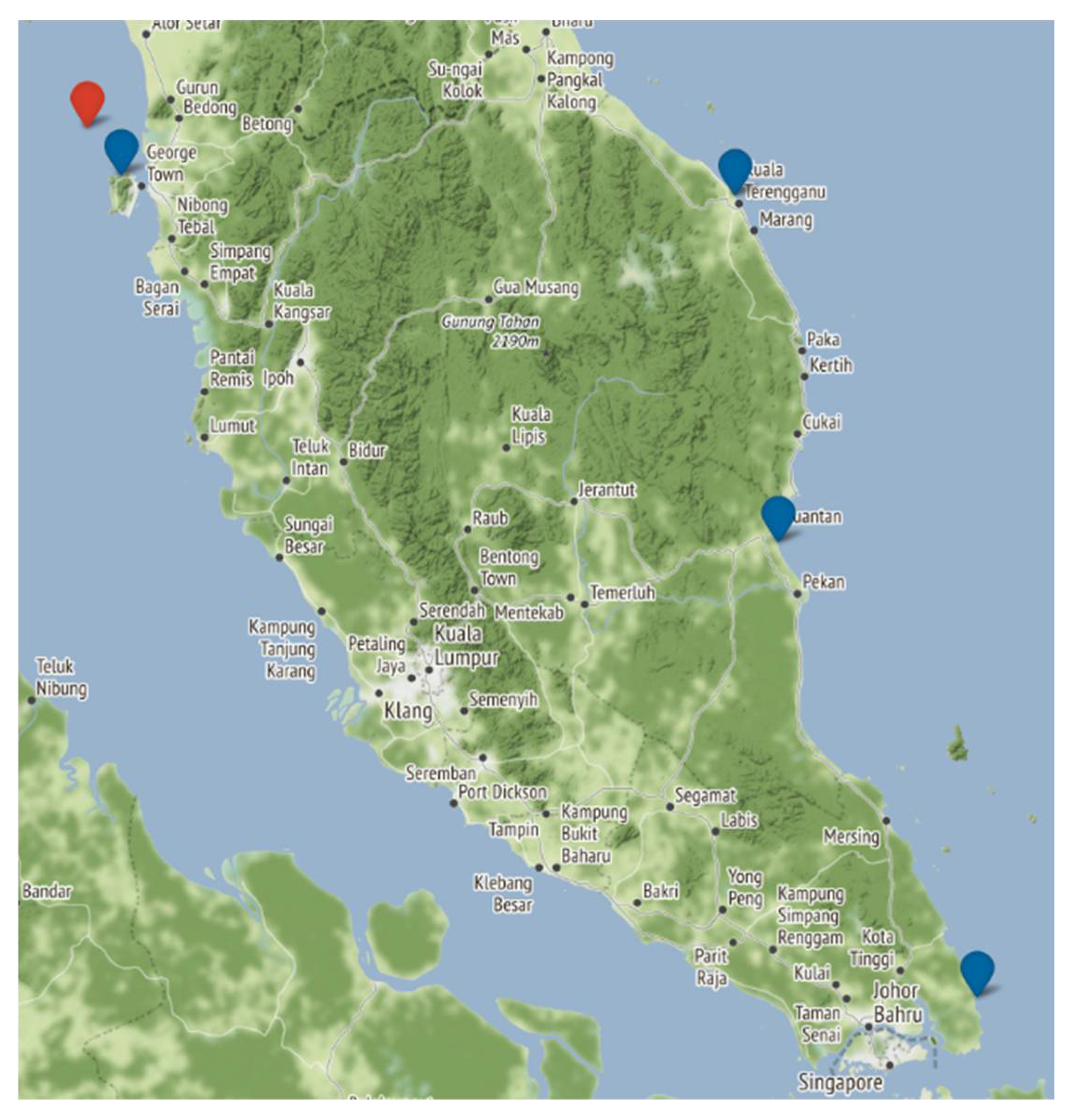

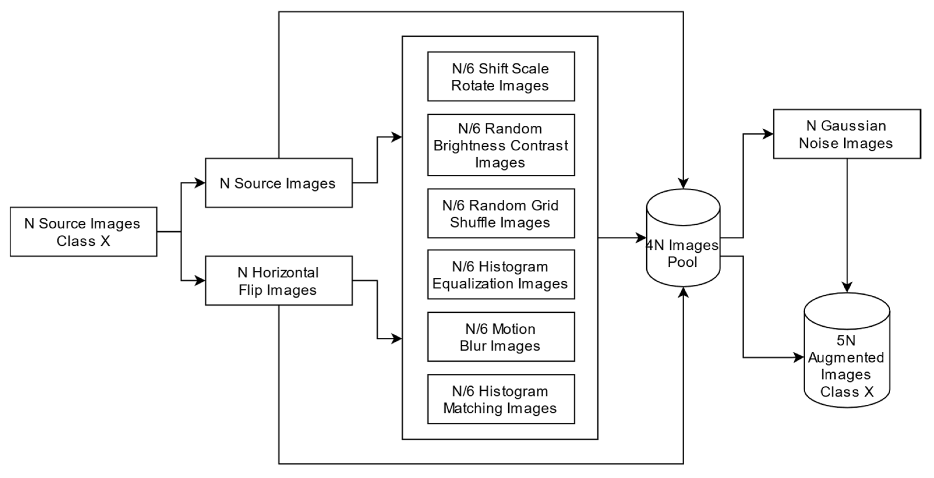
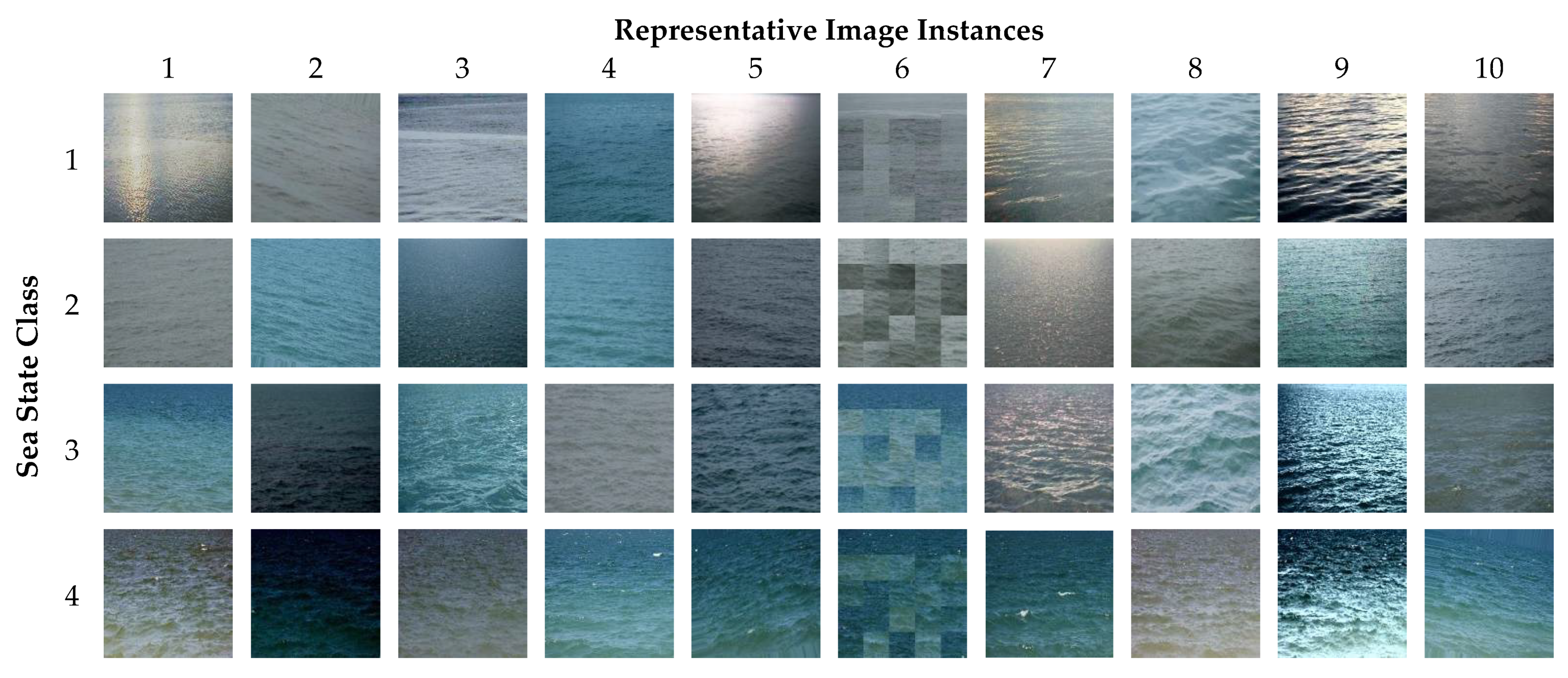
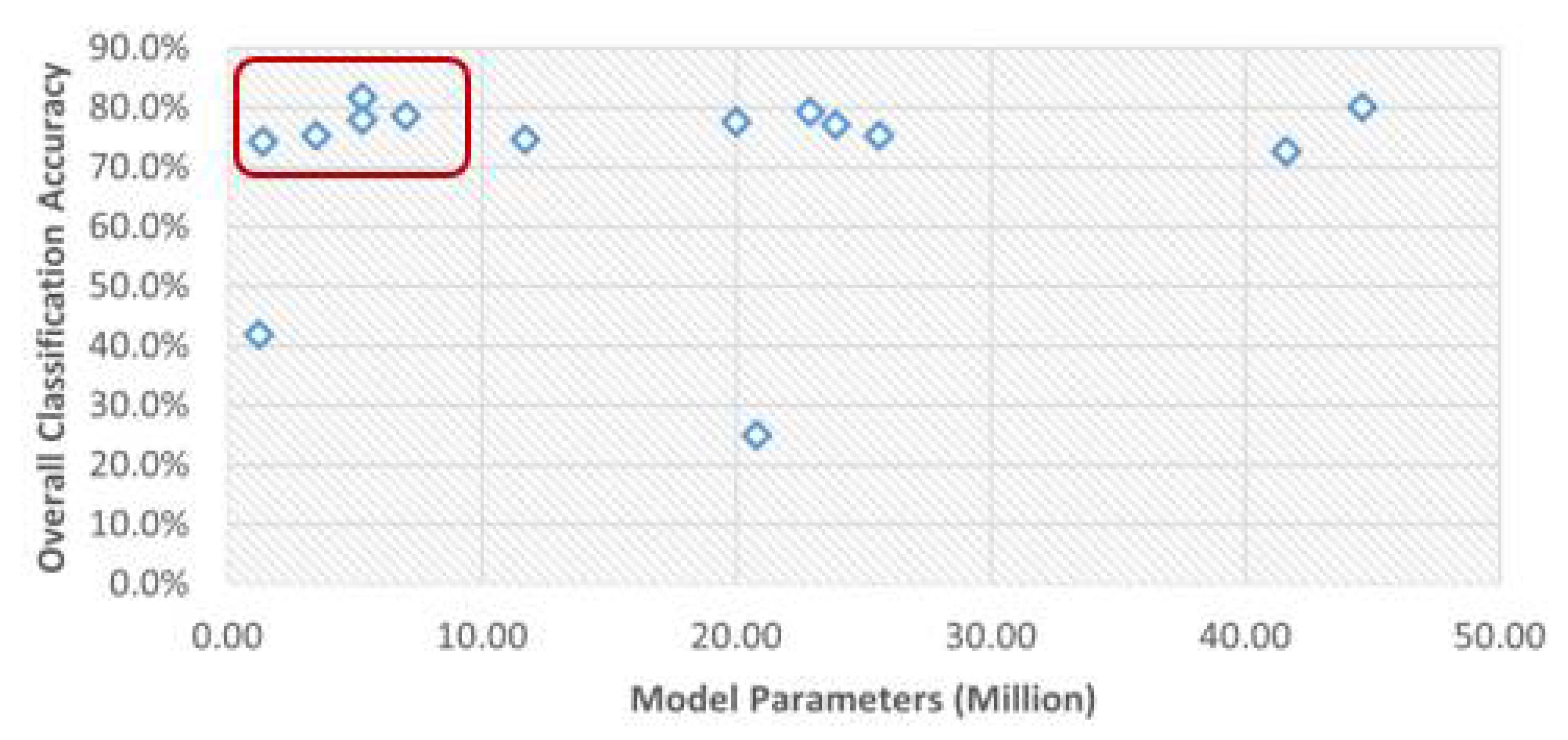

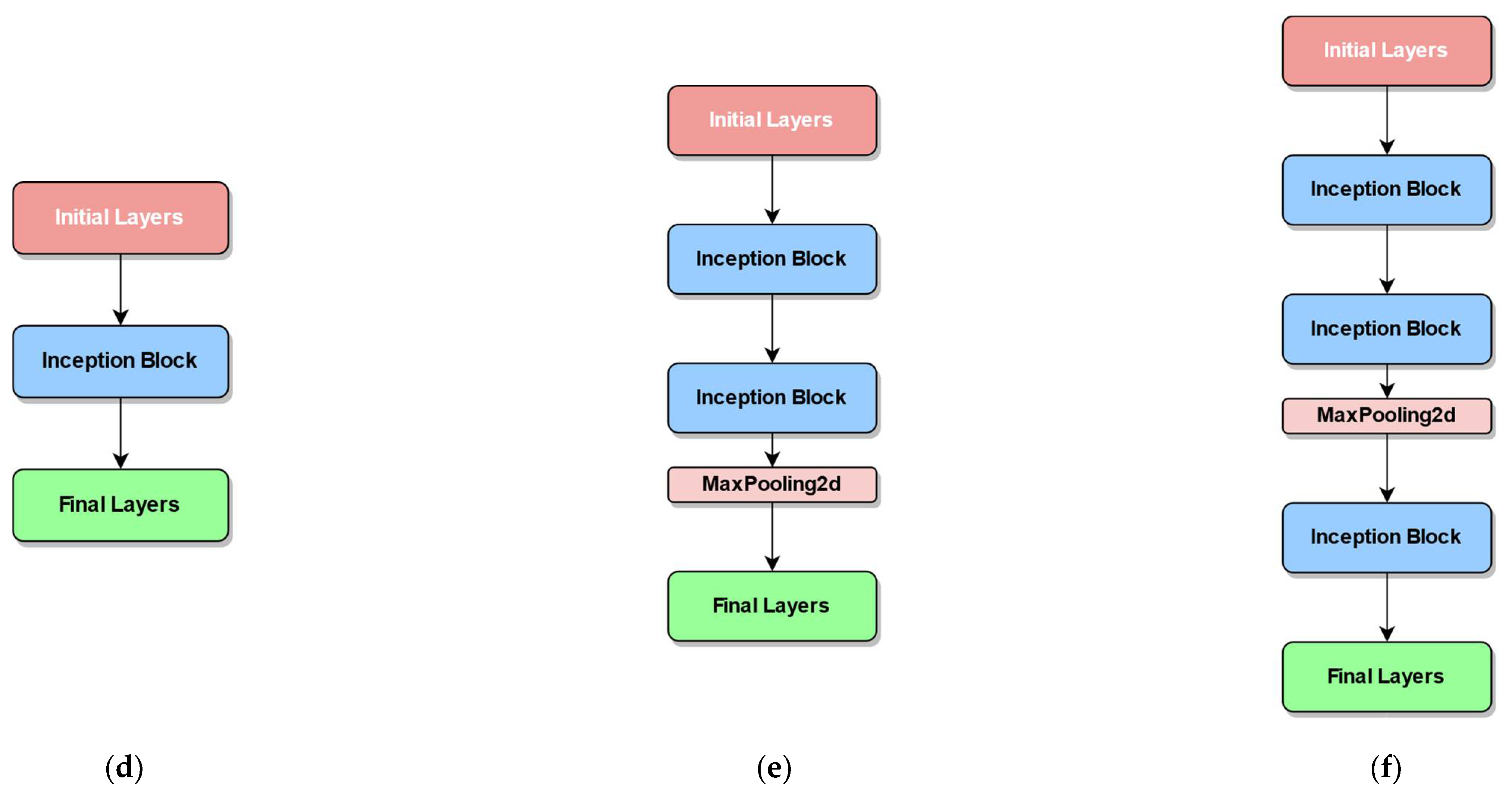
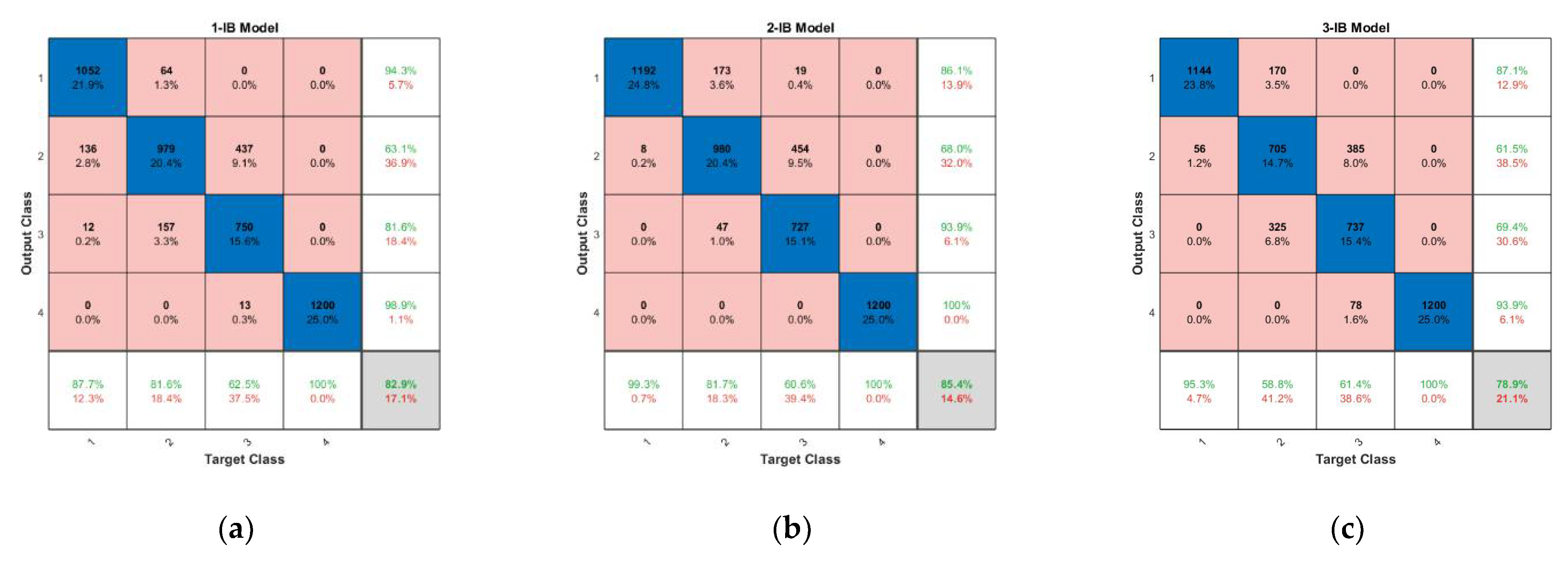
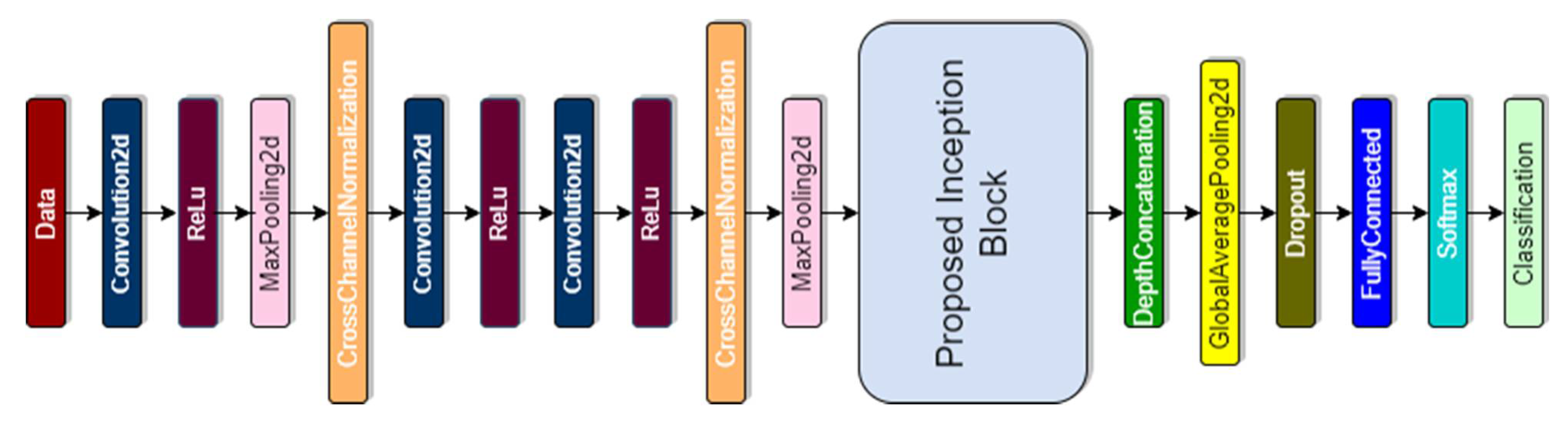
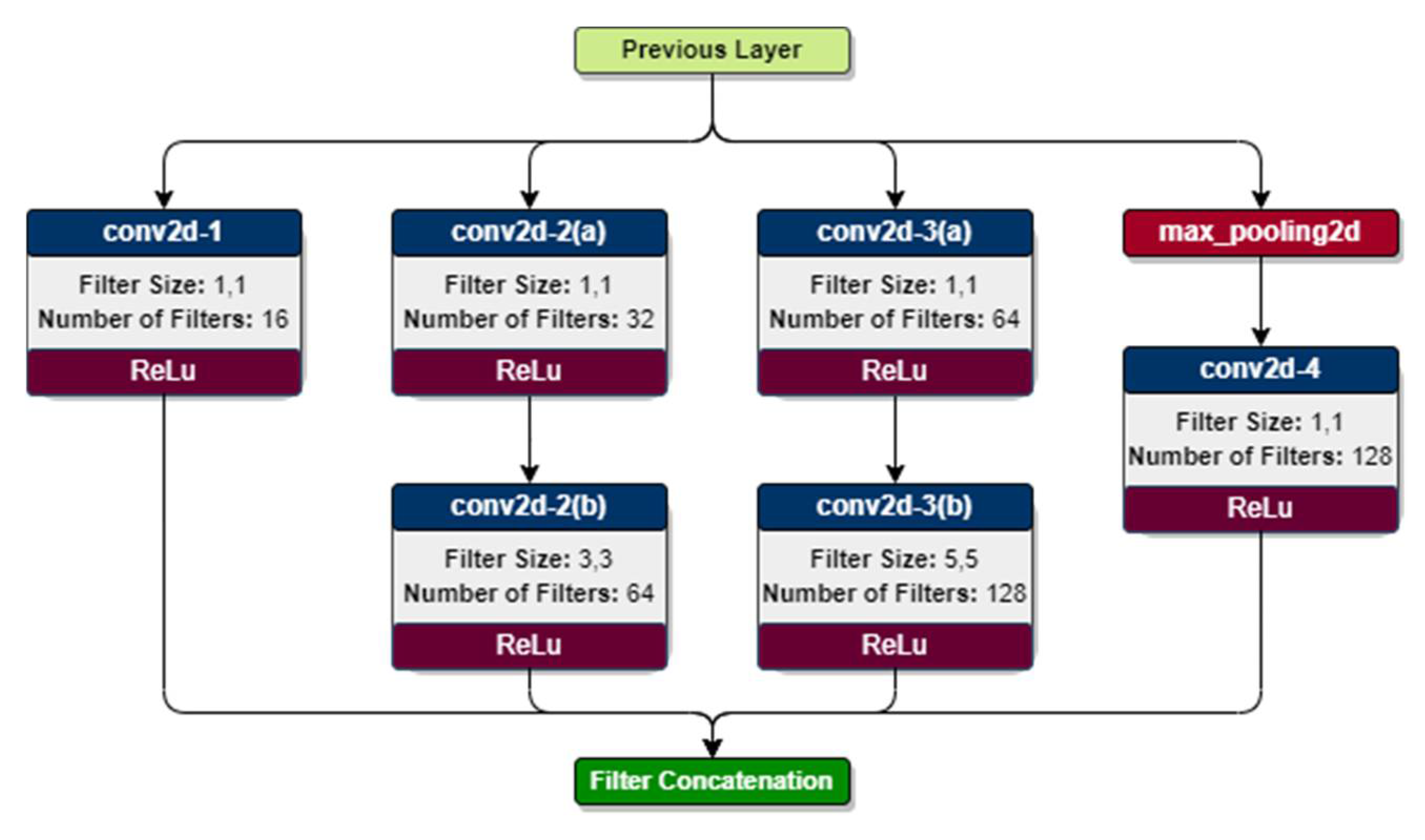
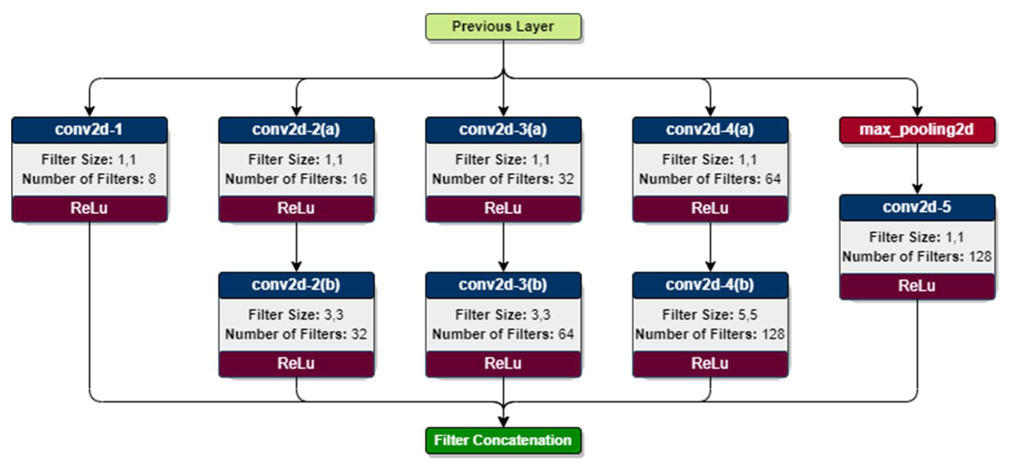
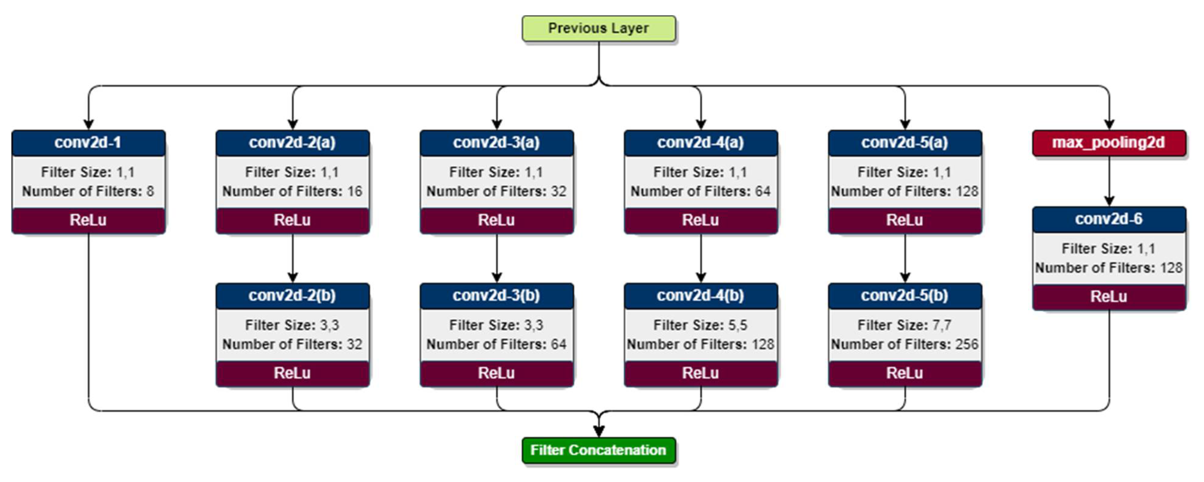

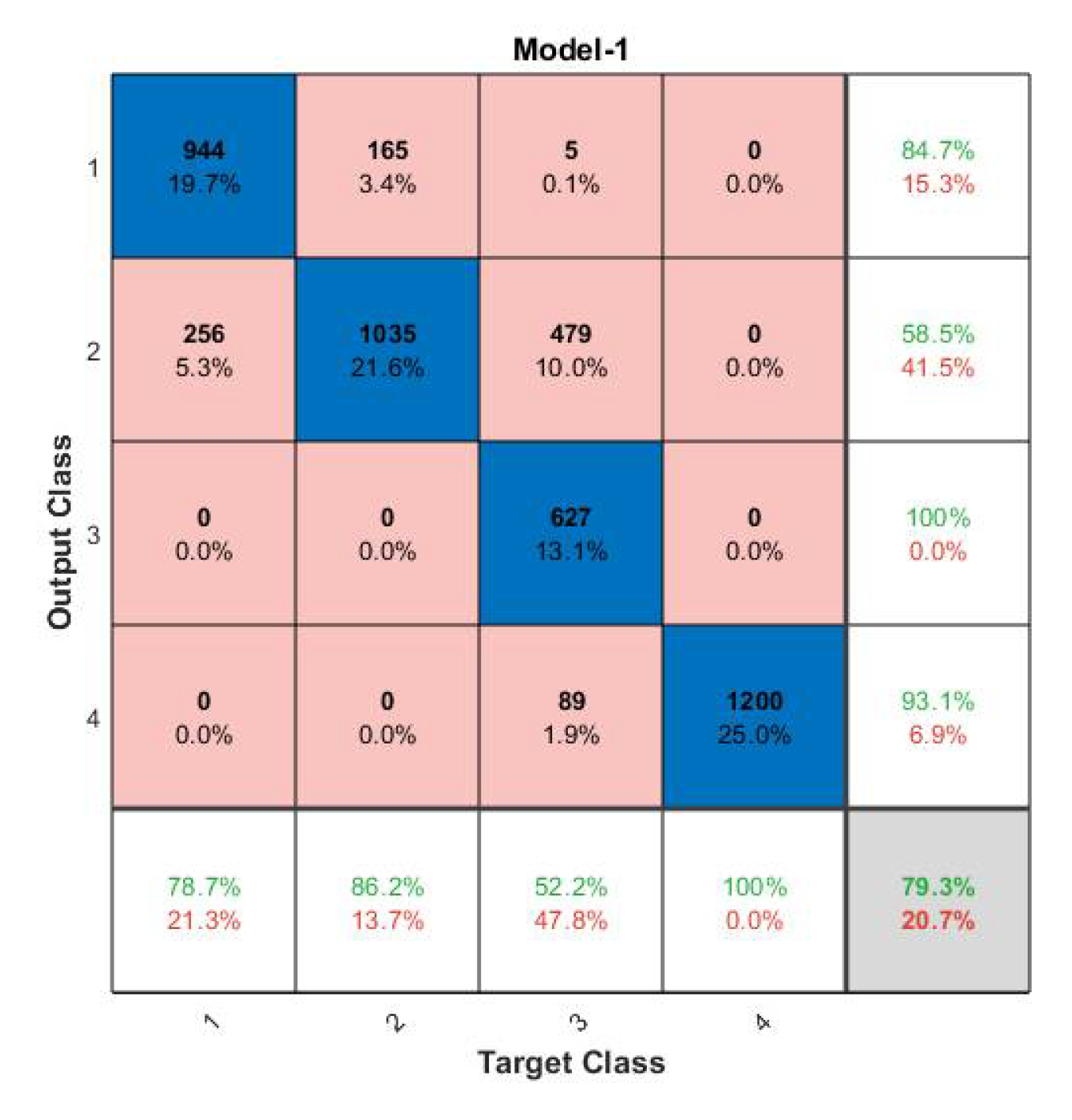

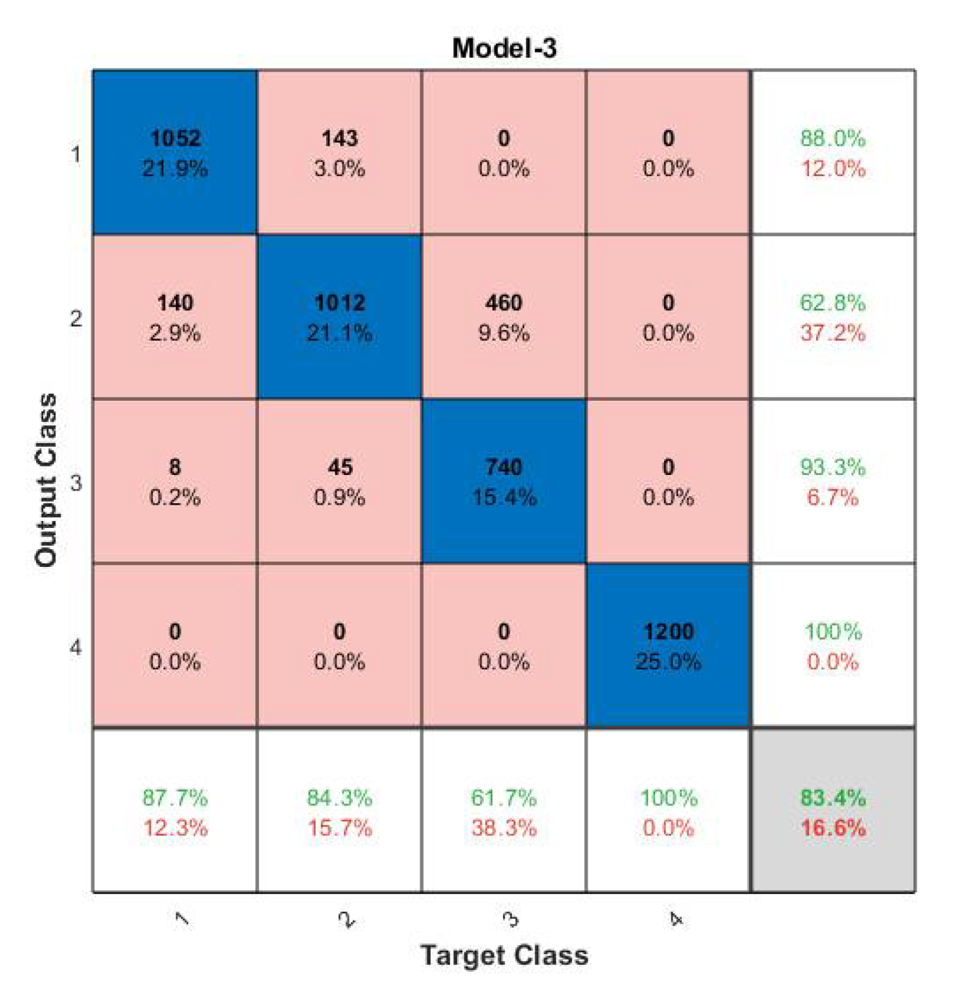
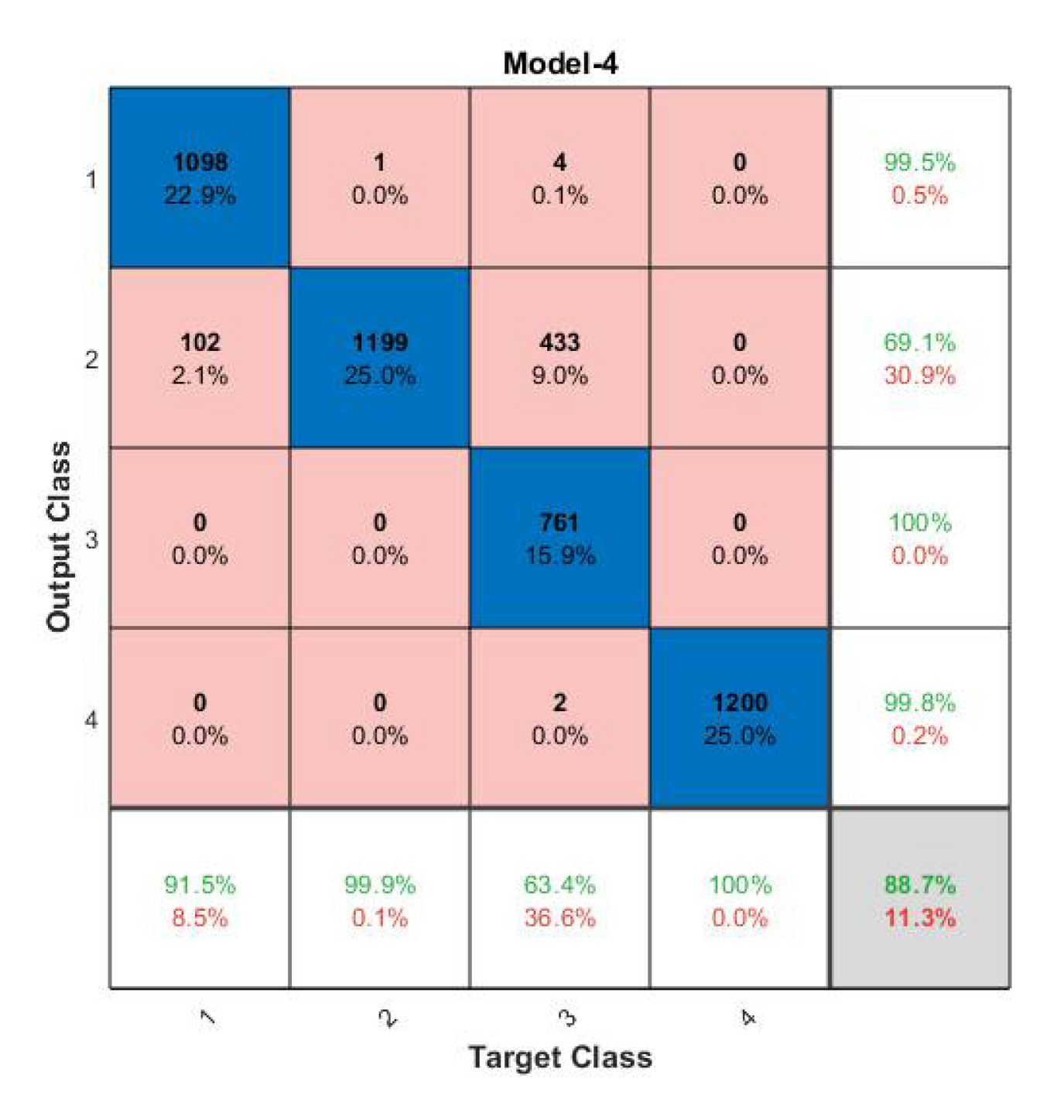


Publisher’s Note: MDPI stays neutral with regard to jurisdictional claims in published maps and institutional affiliations. |
© 2022 by the authors. Licensee MDPI, Basel, Switzerland. This article is an open access article distributed under the terms and conditions of the Creative Commons Attribution (CC BY) license (https://creativecommons.org/licenses/by/4.0/).