
Microclimatic Evaluation of Five Types of Colombian Greenhouses Using Geostatistical Techniques


Abstract
:1. Introduction
2. Materials and Methods
2.1. Description and Location of the Greenhouses
2.1.1. Traditional Greenhouse (TG)
2.1.2. Multi-Tunnel Greenhouse (MG)
2.1.3. Hanging Type Greenhouse (HG)
2.1.4. Spatial Greenhouse (SG)
2.2. Monitoring and Recording of Microclimatic Data
2.3. Geostatistical Analysis
2.3.1. Exploratory Analysis Phase
2.3.2. Structural Analysis Phase
2.3.3. Prediction Phase
3. Results and Discussions
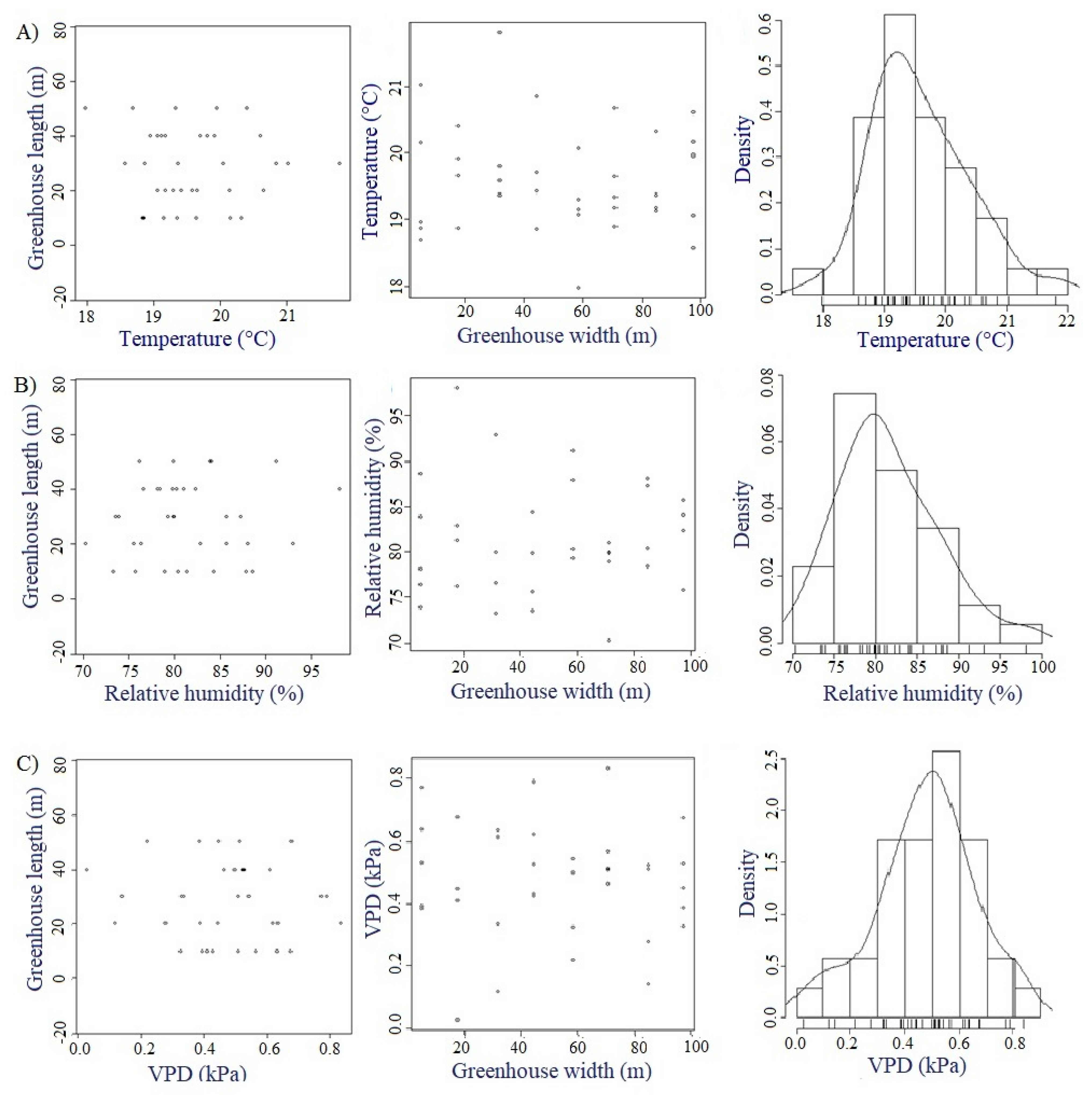
3.1. Exploratory Analysis
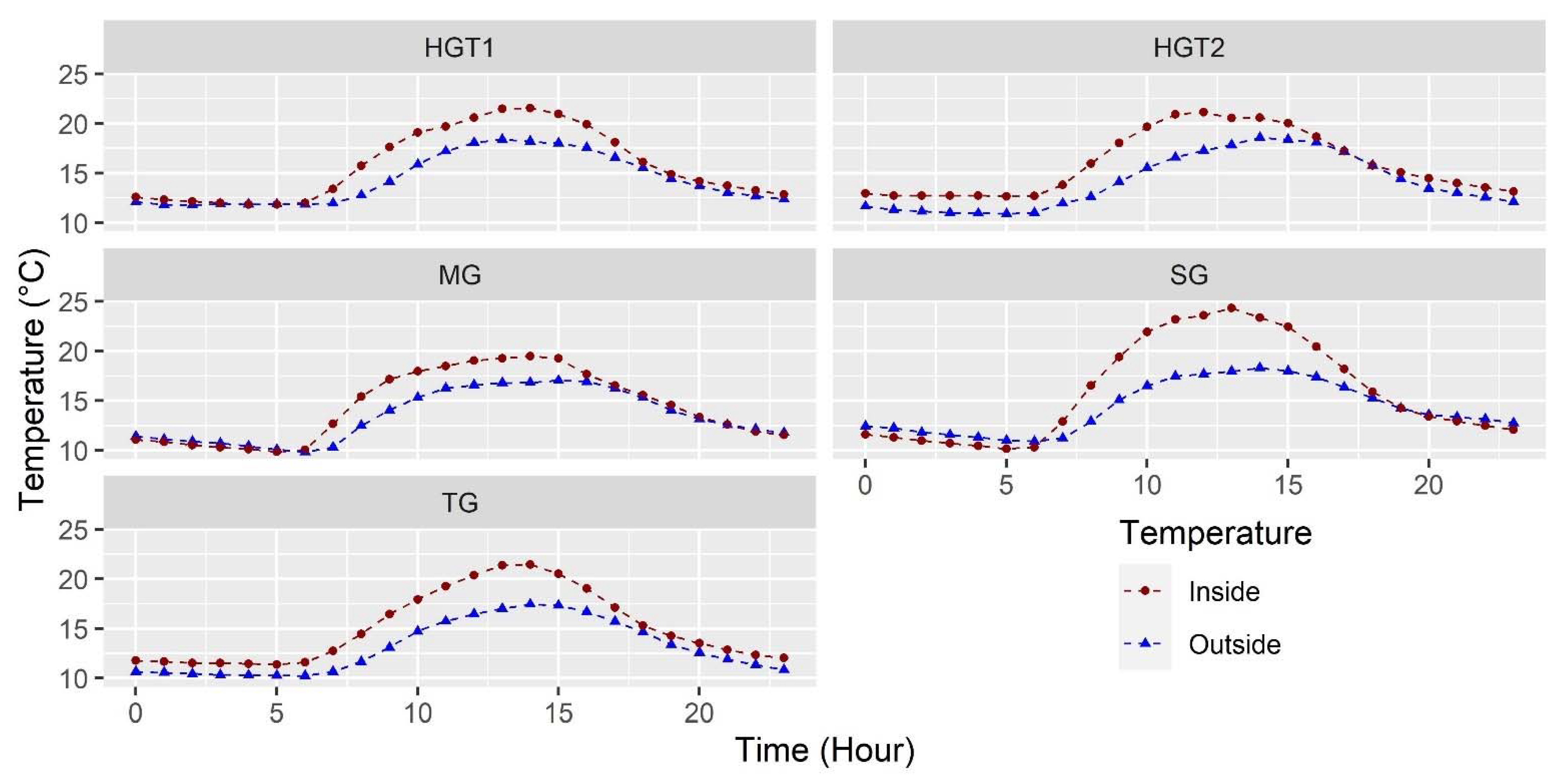
3.1.1. Temperature
3.1.2. Relative Humidity
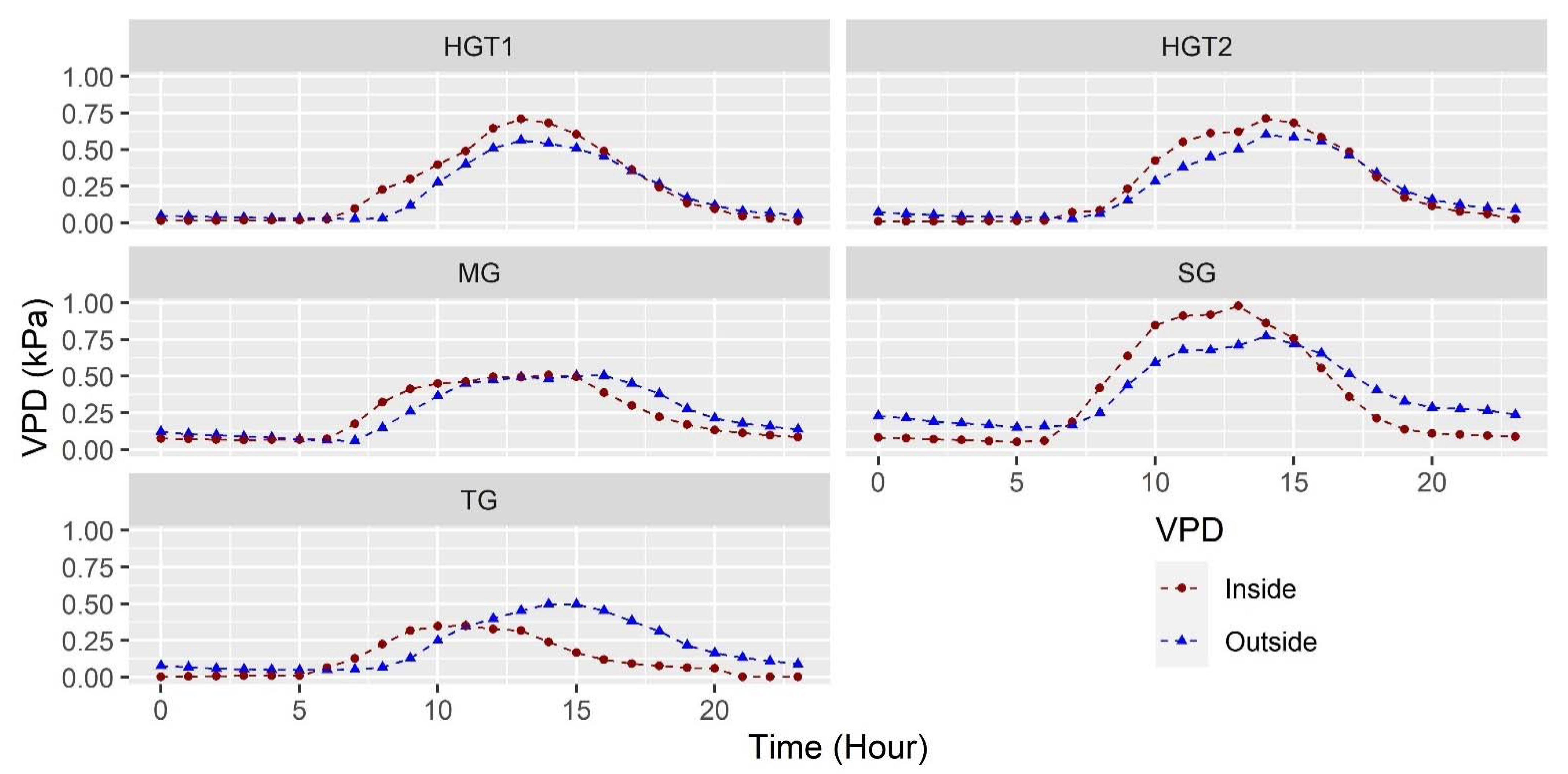
3.1.3. Vapor Pressure Deficit (VPD)
3.1.4. Solar Radiation
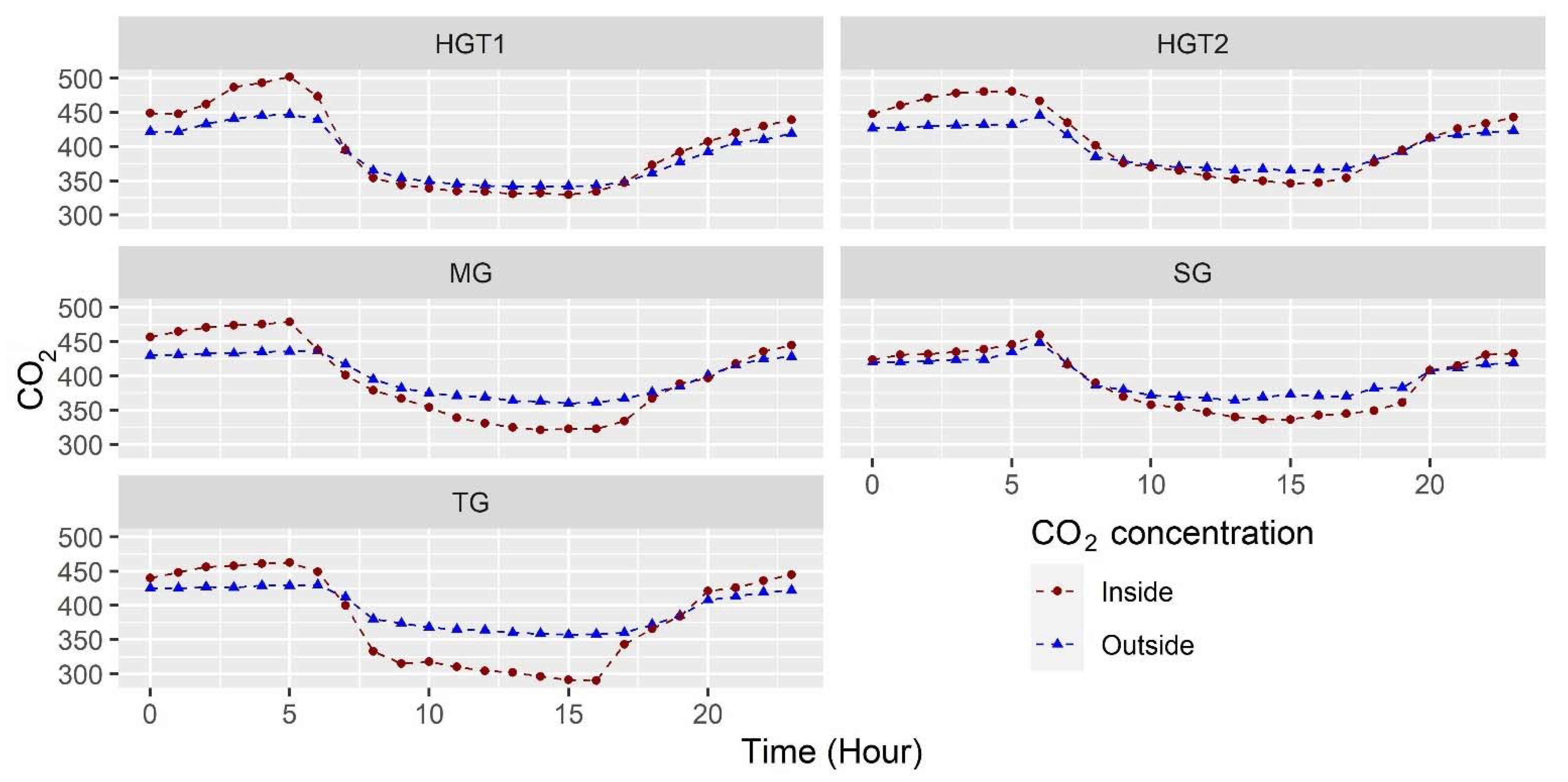
3.1.5. Carbon Dioxide (CO2) Concentration
3.1.6. Testing of Geostatistical Assumptions
3.2. Structural Analysis
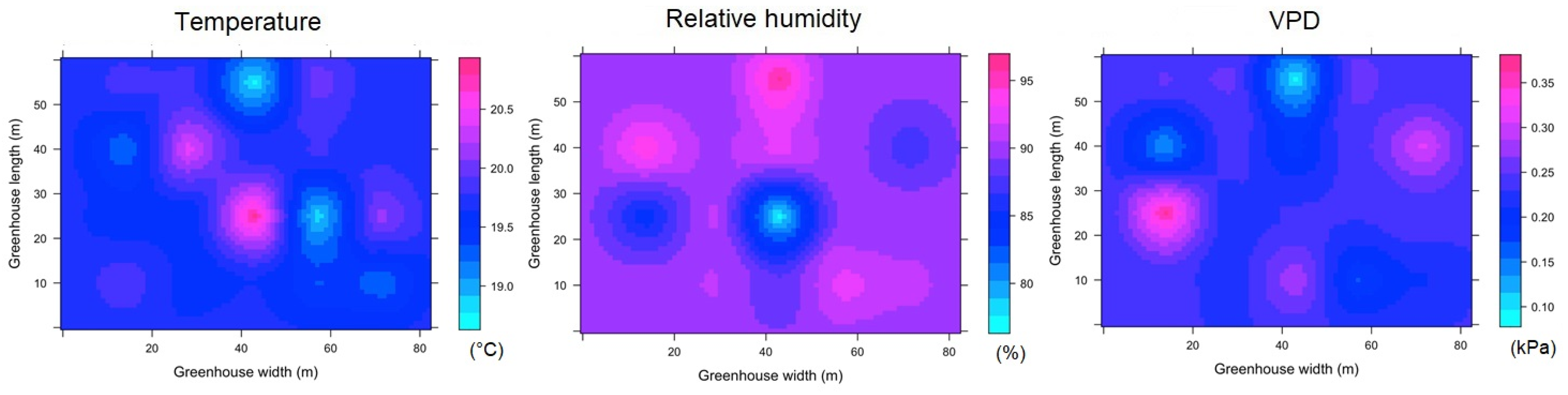
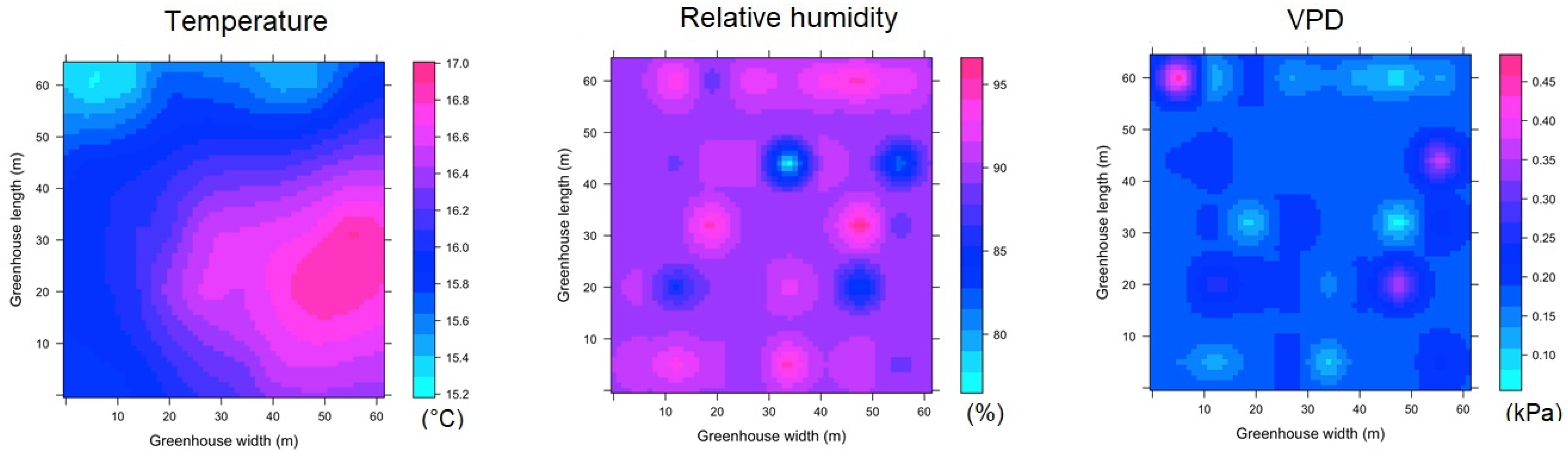
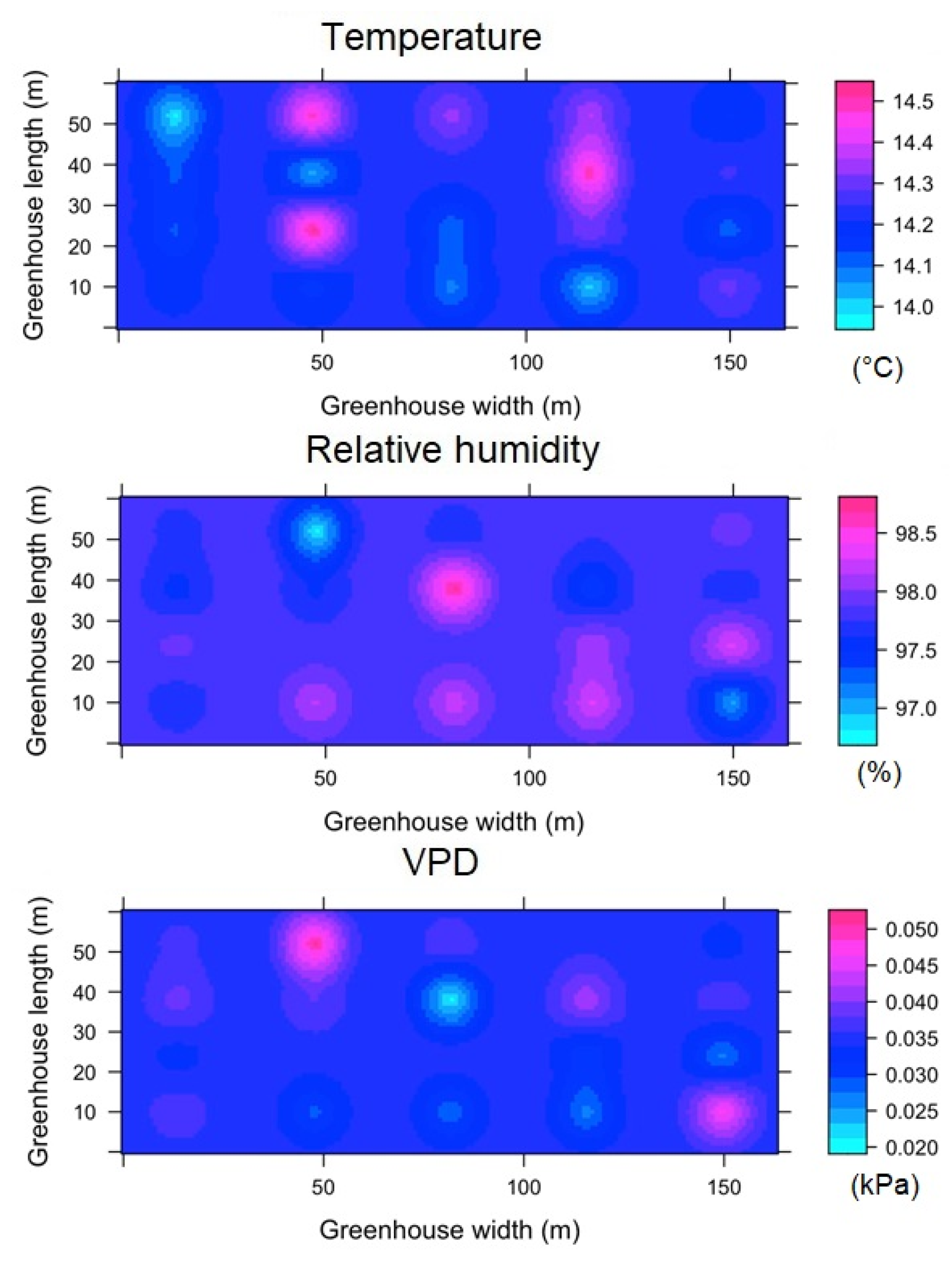
3.3. Prediction of the Spatial Behavior of the Microclimate
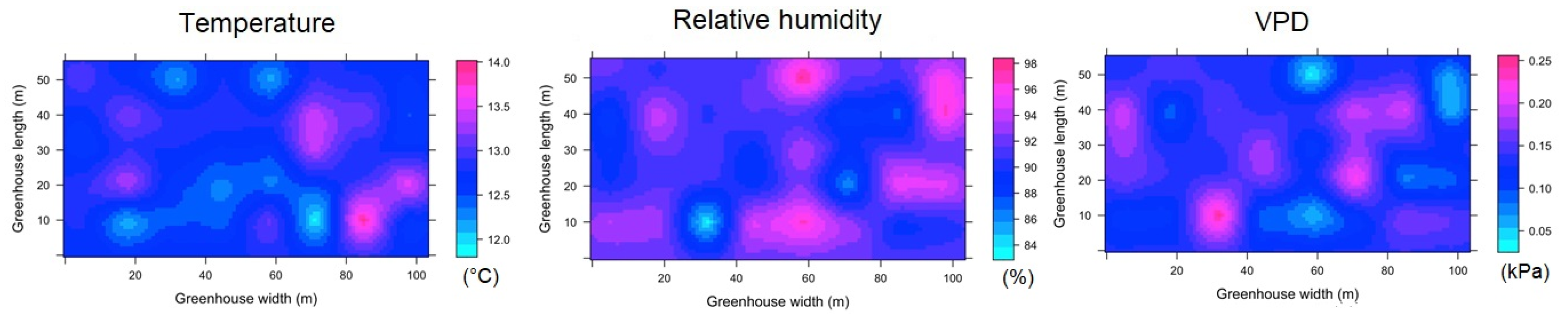
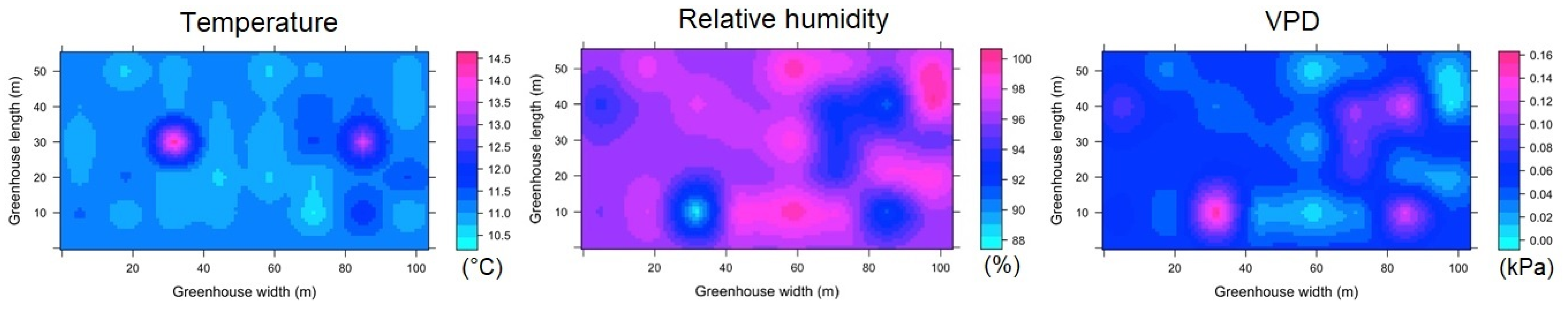
3.3.1. Spatial variability of microclimate in MG
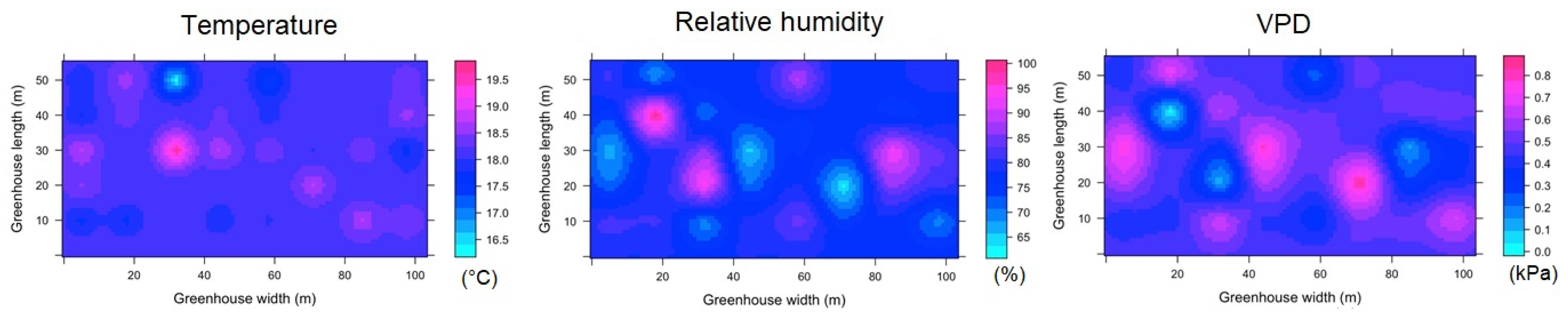
3.3.2. Spatial Variability of Microclimate in TG
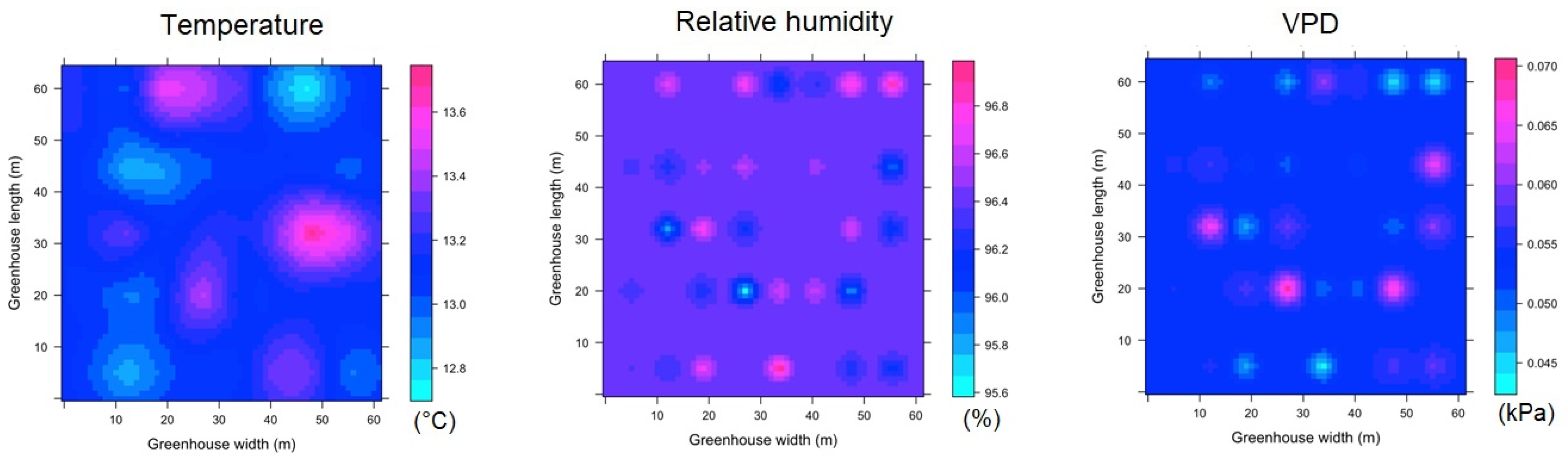
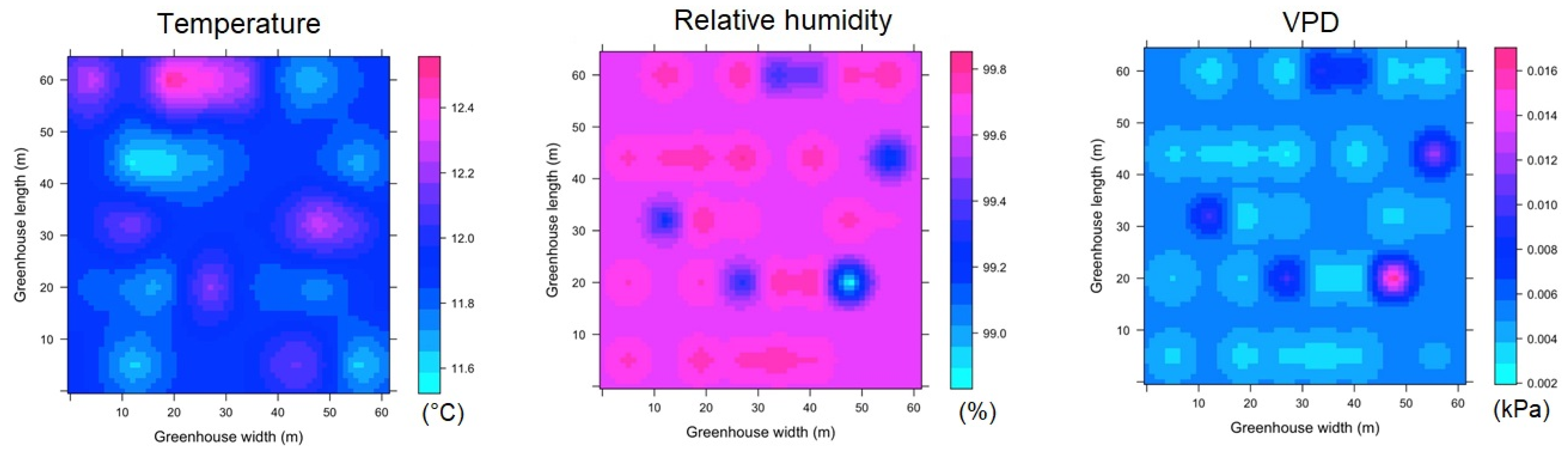
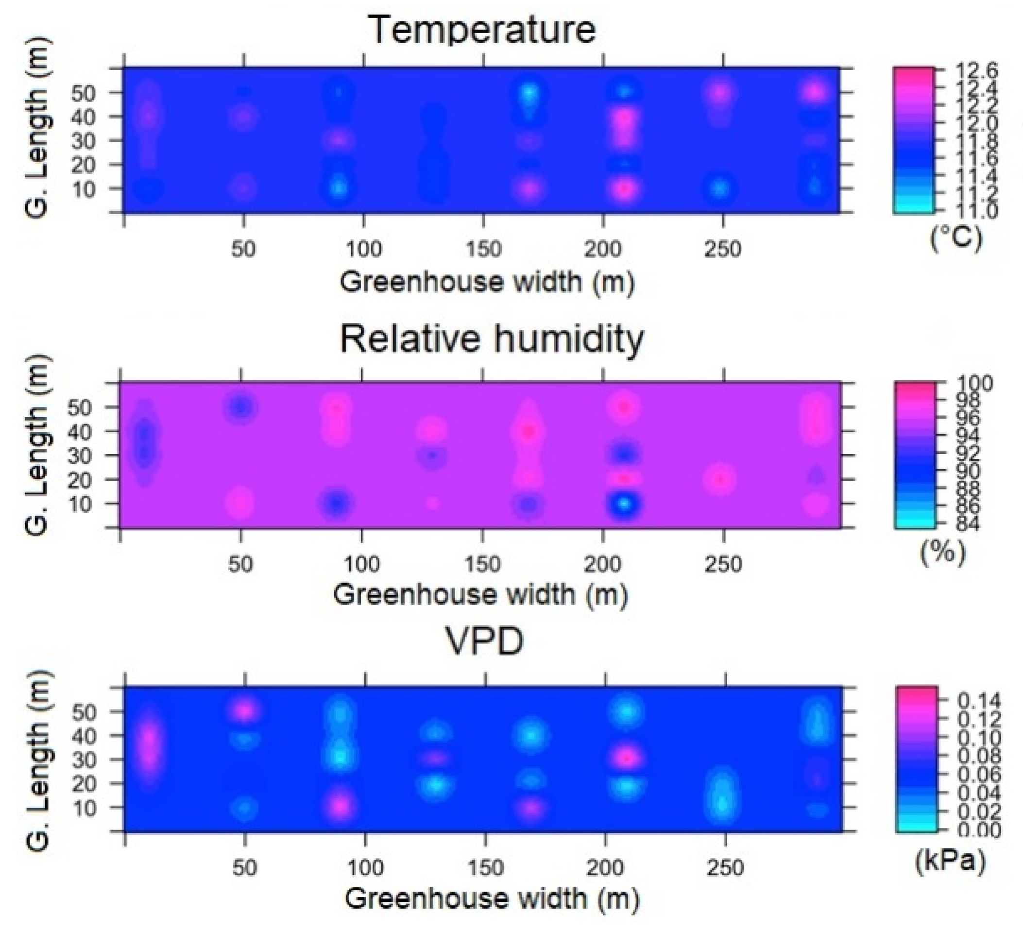
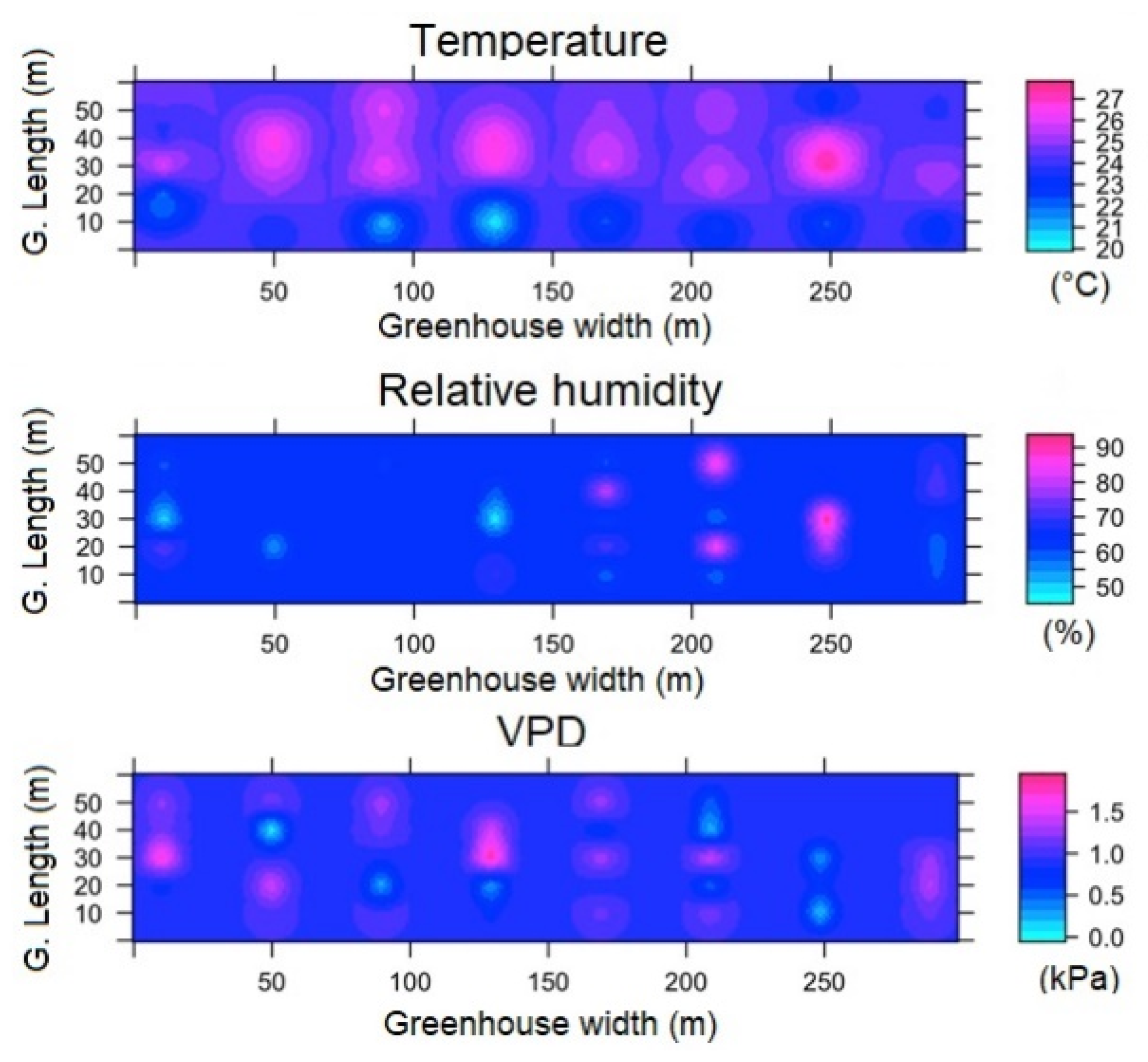
3.3.3. Spatial Variability of Microclimate in SG
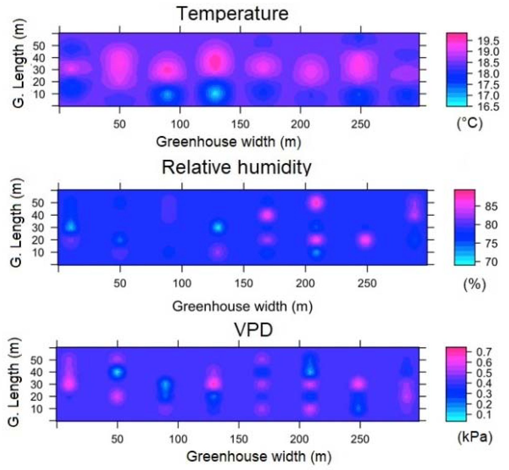
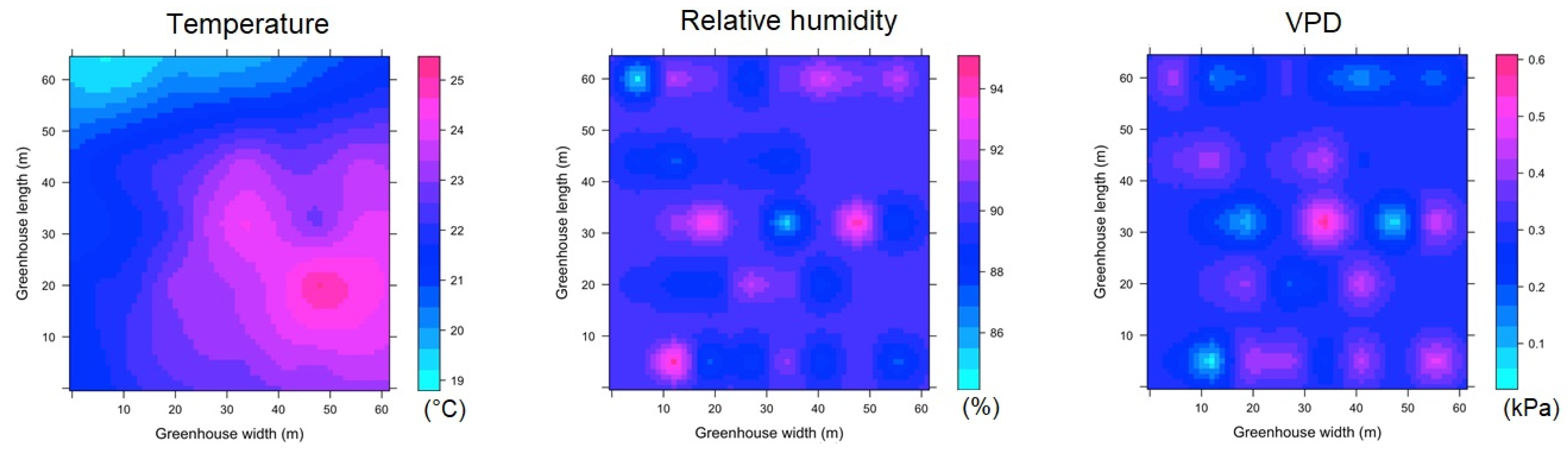
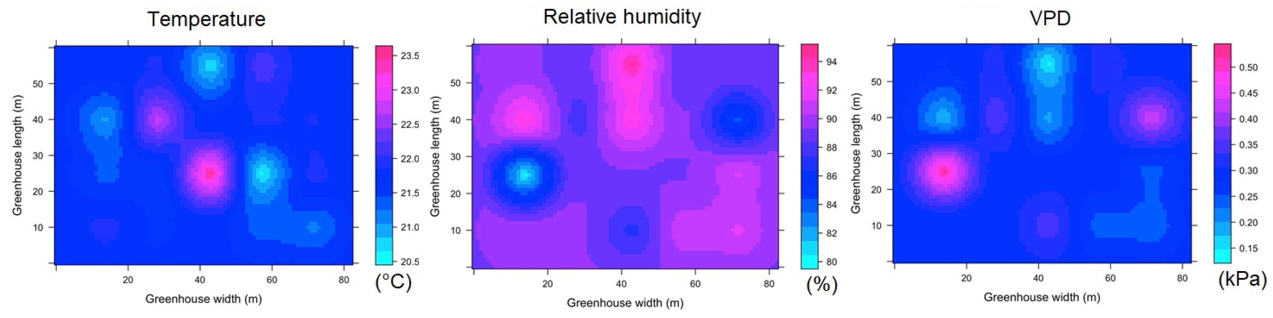
3.3.4. Spatial Variability of Microclimate in HGT1
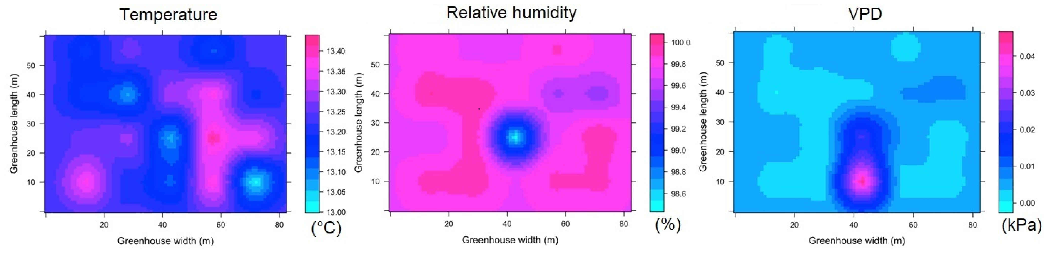
3.3.5. Spatial Variability of Microclimate in HGT2
4. Conclusions
Author Contributions
Funding
Institutional Review Board Statement
Informed Consent Statement
Data Availability Statement
Acknowledgments
Conflicts of Interest
Appendix A


References
- Lee, C.K.; Chung, M.; Shin, K.-Y.; Im, Y.-H.; Yoon, S.-W. A Study of the Effects of Enhanced Uniformity Control of Greenhouse Environment Variables on Crop Growth. Energies 2019, 12, 1749. [Google Scholar] [CrossRef] [Green Version]
- Nicolosi, G.; Volpe, R.; Messineo, A. An Innovative Adaptive Control System to Regulate Microclimatic Conditions in a Greenhouse. Energies 2017, 10, 722. [Google Scholar] [CrossRef] [Green Version]
- Rocha, G.A.O.; Pichimata, M.A.; Villagran, E. Research on the Microclimate of Protected Agriculture Structures Using Numerical Simulation Tools: A Technical and Bibliometric Analysis as a Contribution to the Sustainability of Under-Cover Cropping in Tropical and Subtropical Countries. Sustainability 2021, 13, 10433. [Google Scholar] [CrossRef]
- Soussi, M.; Chaibi, M.T.; Buchholz, M.; Saghrouni, Z. Comprehensive Review on Climate Control and Cooling Systems in Greenhouses under Hot and Arid Conditions. Agronomy 2022, 12, 626. [Google Scholar] [CrossRef]
- Rojas-Rishor, A.; Flores-Velazquez, J.; Villagran, E.; Aguilar-Rodríguez, C.E. Valuation of Climate Performance of a Low-Tech Greenhouse in Costa Rica. Processes 2022, 10, 693. [Google Scholar] [CrossRef]
- Sapounas, A.; Katsoulas, N.; Slager, B.; Bezemer, R.; Lelieveld, C. Design, Control, and Performance Aspects of Semi-Closed Greenhouses. Agronomy 2020, 10, 1739. [Google Scholar] [CrossRef]
- Villagrán, E.; Flores-Velazquez, J.; Akrami, M.; Bojacá, C. Influence of the Height in a Colombian Multi-Tunnel Greenhouse on Natural Ventilation and Thermal Behavior: Modeling Approach. Sustainability 2021, 13, 13631. [Google Scholar] [CrossRef]
- Reynafarje, X.; Villagrán, E.A.; Bojacá, C.R.; Gil, R.; Schrevens, E. Simulation and Validation of the Airflow inside a Naturally Ventilated Greenhouse Designed for Tropical Conditions. Acta Hortic. 2020, 1271, 55–62. [Google Scholar] [CrossRef]
- Villagrán, E.A.; Baeza Romero, E.J.; Bojacá, C.R. Transient CFD Analysis of the Natural Ventilation of Three Types of Greenhouses Used for Agricultural Production in a Tropical Mountain Climate. Biosyst. Eng. 2019, 188, 288–304. [Google Scholar] [CrossRef]
- López, A.; Valera, D.L.; Molina-Aiz, F. Sonic Anemometry to Measure Natural Ventilation in Greenhouses. Sensors 2011, 11, 9820–9838. [Google Scholar] [CrossRef]
- Villagrán-Munar, E.A.; Bojacá-Aldana, C.R. CFD Simulation of the Increase of the Roof Ventilation Area in a Traditional Colombian Greenhouse: Effect on Air Flow Patterns and Thermal Behavior. Int. J. Heat Technol. 2019, 37, 881–892. [Google Scholar] [CrossRef]
- Bojacá, C.R.; Gil, R.; Gómez, S.; Cooman, A.; Schrevens, E. Analysis of Greenhouse Air Temperature Distribution Using Geostatistical Methods. Trans. ASABE 2009, 52, 957. [Google Scholar] [CrossRef]
- Moon, T.; Lee, J.W.; Son, J.E. Accurate Imputation of Greenhouse Environment Data for Data Integrity Utilizing Two-Dimensional Convolutional Neural Networks. Sensors 2021, 21, 2187. [Google Scholar] [CrossRef] [PubMed]
- Li, K.; Xue, W.; Mao, H.; Chen, X.; Jiang, H.; Tan, G. Optimizing the 3D Distributed Climate inside Greenhouses Using Multi-Objective Optimization Algorithms and Computer Fluid Dynamics. Energies 2019, 12, 2873. [Google Scholar] [CrossRef] [Green Version]
- Riahi, J.; Vergura, S.; Mezghani, D.; Mami, A. Intelligent Control of the Microclimate of an Agricultural Greenhouse Powered by a Supporting PV System. Appl. Sci. 2020, 10, 1350. [Google Scholar] [CrossRef] [Green Version]
- Balendonck, J.; Sapounas, A.A.; Kempkes, F.; Van Os, E.A.; Van Der Schoor, R.; Van Tuijl, B.A.J.; Keizer, L.C.P. Using a Wireless Sensor Network to Determine Climate Heterogeneity of a Greenhouse Environment. Acta Hortic. 2014, 1037, 539–546. [Google Scholar] [CrossRef]
- Saberian, A.; Sajadiye, S.M. The Effect of Dynamic Solar Heat Load on the Greenhouse Microclimate Using CFD Simulation. Renew. Energy 2019, 138, 722–737. [Google Scholar] [CrossRef]
- Ma, D.; Carpenter, N.; Maki, H.; Rehman, T.U.; Tuinstra, M.R.; Jin, J. Greenhouse Environment Modeling and Simulation for Microclimate Control. Comput. Electron. Agric. 2019, 162, 134–142. [Google Scholar] [CrossRef]
- Taki, M.; Ajabshirchi, Y.; Ranjbar, S.F.; Rohani, A.; Matloobi, M. Modeling and Experimental Validation of Heat Transfer and Energy Consumption in an Innovative Greenhouse Structure. Inf. Process. Agric. 2016, 3, 157–174. [Google Scholar] [CrossRef] [Green Version]
- Vanthoor, B.H.E.; Gázquez, J.C.; Magán, J.J.; Ruijs, M.N.A.; Baeza, E.; Stanghellini, C.; van Henten, E.J.; de Visser, P.H.B. A Methodology for Model-Based Greenhouse Design: Part 4, Economic Evaluation of Different Greenhouse Designs: A Spanish Case. Biosyst. Eng. 2012, 111, 336–349. [Google Scholar] [CrossRef]
- Baeza, E.J.; Pérez-Parra, J.; Montero, J.I. Effect of Ventilator Size on Natural Ventilation in Parral Greenhouse by Means of CFD Simulations. In Proceedings of the International Conference on Sustainable Greenhouse Systems: Greensys2004, Leuven, Belgium, 12–16 September 2004; pp. 465–472. [Google Scholar] [CrossRef] [Green Version]
- Bazgaou, A.; Fatnassi, H.; Bouhroud, R.; Gourdo, L.; Ezzaeri, K.; Tiskatine, R.; Demrati, H.; Wifaya, A.; Bekkaoui, A.; Aharoune, A.; et al. An Experimental Study on the Effect of a Rock-Bed Heating System on the Microclimate and the Crop Development under Canarian Greenhouse. Sol. Energy 2018, 176, 42–50. [Google Scholar] [CrossRef]
- Piscia, D.; Muñoz, P.; Panadès, C.; Montero, J.I. A Method of Coupling CFD and Energy Balance Simulations to Study Humidity Control in Unheated Greenhouses. Comput. Electron. Agric. 2015, 115, 129–141. [Google Scholar] [CrossRef]
- Majdoubi, H.; Boulard, T.; Fatnassi, H.; Senhaji, A.; Elbahi, S.; Demrati, H.; Mouqallid, M.; Bouirden, L. Canary Greenhouse CFD Nocturnal Climate Simulation. Open J. Fluid Dyn. 2016, 6, 88–100. [Google Scholar] [CrossRef] [Green Version]
- Katsoulas, N.; Kittas, C. Impact of Greenhouse Microclimate on Plant Growth and Development with Special Reference to the Solanaceae. Eur. J. Plant Sci. Biotechnol. 2008, 2, 31–44. [Google Scholar]
- Bakker, J.C. Greenhouse Climate Control: Constraints and Limitations. Greenh. Environ. Control Autom. 1994, 399, 25–36. [Google Scholar] [CrossRef]
- Cheng, X.; Li, D.; Shao, L.; Ren, Z. A Virtual Sensor Simulation System of a Flower Greenhouse Coupled with a New Temperature Microclimate Model Using Three-Dimensional CFD. Comput. Electron. Agric. 2021, 181, 105934. [Google Scholar] [CrossRef]
- Huang, Y.; Jin, Y.; Zhang, K.; Yang, S. A Method to Measure Humidity Based on Dry-Bulb and Wet-Bulb Temperatures. Res. J. Appl. Sci. Eng. Technol. 2013, 6, 2984–2987. [Google Scholar] [CrossRef]
- Diggle, P.J.; Menezes, R.; Su, T. Geostatistical Inference under Preferential Sampling. J. R. Stat. Soc. Ser. C (Appl. Stat.) 2010, 59, 191–232. [Google Scholar] [CrossRef]
- Hengl, T. Practical Guide to Geostatistical Mapping; Office for Official Publications of the European Communities: Luxembourg, 2009; pp. 1–293. [Google Scholar]
- Kyriakidis, P.C.; Journel, A.G. Geostatistical Space–Time Models: A Review. Math. Geol. 1999, 31, 651–684. [Google Scholar] [CrossRef]
- O’Hanlon, S.J.; Slater, H.C.; Cheke, R.A.; Boatin, B.A.; Coffeng, L.E.; Pion, S.D.S.; Boussinesq, M.; Zouré, H.G.M.; Stolk, W.A.; Basáñez, M.-G. Model-Based Geostatistical Mapping of the Prevalence of Onchocerca Volvulus in West Africa. PLoS Negl. Trop. Dis. 2016, 10, e0004328. [Google Scholar] [CrossRef] [Green Version]
- Oliver, M.A. An Overview of Geostatistics and Precision Agriculture. In Geostatistical Applications for Precision Agriculture; Springer: Berlin/Heidelberg, Germany, 2010; pp. 1–34. [Google Scholar]
- Reid, A. Greenhouse Roses for Cutflower Production; Department of Primary Industries and Regional Development: Perth, Australia, 2008; p. 1. [Google Scholar]
- Piscia, D.; Montero, J.I.; Baeza, E.; Bailey, B.J. A CFD Greenhouse Night-Time Condensation Model. Biosyst. Eng. 2012, 111, 141–154. [Google Scholar] [CrossRef]
- Villagrán, M.E.A.; Bojacá, A.C.R. Numerical Evaluation of Passive Strategies for Nocturnal Climate Optimization in a Greenhouse Designed for Rose Production (Rosa Spp.). Ornam. Hortic. 2019, 25, 351–364. [Google Scholar] [CrossRef] [Green Version]
- Villagrán-Munar, E.A.; Bojacá-Aldana, C.R. Study Using a CFD Approach of the Efficiency of a Roof Ventilation Closure System in a Multi-Tunnel Greenhouse for Nighttime Microclimate Optimization. Rev. Ceres 2020, 67, 345–356. [Google Scholar] [CrossRef]
- Bouhoun Ali, H.; Bournet, P.E.; Danjou, V.; Morille, B.; Migeon, C. CFD Simulations of the Night-Time Condensation inside a Closed Glasshouse: Sensitivity Analysis to Outside External Conditions, Heating and Glass Properties. Biosyst. Eng. 2014, 127, 159–175. [Google Scholar] [CrossRef]
- Amani, M.; Foroushani, S.; Sultan, M.; Bahrami, M. Comprehensive Review on Dehumidification Strategies for Agricultural Greenhouse Applications. Appl. Therm. Eng. 2020, 181, 115979. [Google Scholar] [CrossRef]
- Bautista Silva, J.P.; Barbosa, H.; Uribe Vélez, D. Prototipo de Formulación a Base de Rhodotorula Mucilaginosa Para El Control de Botrytis Cinerea En Rosas. Rev. Colomb. Biotecnol. 2016, 18, 13. [Google Scholar] [CrossRef]
- Villagran, E.; Bojacá, C. Analysis of the Microclimatic Behavior of a Greenhouse Used to Produce Carnation (Dianthus caryophyllus L.). Ornam. Hortic. 2020, 26, 109–204. [Google Scholar] [CrossRef]
- Sultan, M.; Miyazaki, T.; Saha, B.B.; Koyama, S. Steady-State Investigation of Water Vapor Adsorption for Thermally Driven Adsorption Based Greenhouse Air-Conditioning System. Rene. Energy 2016, 86, 785–795. [Google Scholar] [CrossRef]
- Shamshiri, R.R.; Jones, J.W.; Thorp, K.R.; Ahmad, D.; Man, H.C.; Taheri, S. Review of Optimum Temperature, Humidity, and Vapour Pressure Deficit for Microclimate Evaluation and Control in Greenhouse Cultivation of Tomato: A Review. Int. Agrophys. 2018, 32, 287–302. [Google Scholar] [CrossRef]
- Santosh, D.T.; Tiwari, K.N.; Singh, V.K.; Reddy, A.R.G. Micro Climate Control in Greenhouse. Int. J. Curr. Microbiol. Appied Sci. 2017, 6, 1730–1742. [Google Scholar]
- Konopacki, P.J.; Treder, W.; Klamkowski, K. Comparison of Vapour Pressure Deficit Patterns during Cucumber Cultivation in a Traditional High PE Tunnel Greenhouse and a Tunnel Greenhouse Equipped with a Heat Accumulator. Span. J. Agric. Res. 2018. [Google Scholar] [CrossRef]
- Domis, M.; Papadopoulos, A.P.; Gosselin, A. Greenhouse Tomato Fruit Quality. Hortic. Rev. 2002, 26, 239–349. [Google Scholar]
- Baudoin, W.; Nono-Womdim, R.; Lutaladio, N.; Hodder, A.; Castilla, N.; Leonardi, C.; De Pascale, S.; Qaryouti, M. Good Agricultural Practices for Greenhouse Vegetable Crops—Principles for Meditterranean Climate Areas; FAO: Rome, Italy, 2013. [Google Scholar]
- Gadhesaria, G.; Desai, C.; Bhatt, R.; Salah, B. Thermal Analysis and Experimental Validation of Environmental Condition inside Greenhouse in Tropicalwet and Dry Climate. Sustainability 2020, 12, 8171. [Google Scholar] [CrossRef]
- Singh, H.; Poudel, M.R.; Dunn, B.L.; Fontanier, C.; Kakani, G. Effect of Greenhouse CO2 Supplementation on Yield and Mineral Element Concentrations of Leafy Greens Grown Using Nutrient Film Technique. Agronomy 2020, 10, 323. [Google Scholar] [CrossRef] [Green Version]
- Vox, G.; Teitel, M.; Pardossi, A.; Minuto, A.; Tinivella, F.; Schettini, E. Sustainable Greenhouse Systems. In Sustainable Agriculture: Technology, Planning and Management (Agriculture Issues and Policies); Salazar, A., Rios, I., Eds.; Nova Science Pub Inc.: New York, NY, USA, 2010; pp. 1–78. [Google Scholar]
- Vadiee, A.; Martin, V. Energy Management in Horticultural Applications through the Closed Greenhouse Concept, State of the Art. Renew. Sustain. Energy Rev. 2012, 16, 5087–5100. [Google Scholar] [CrossRef]
- Garcia, F.J.M. Analysis of the Spatio–Temporal Distribution of Helicoverpa Armigera Hb. in a Tomato Field Using a Stochastic Approach. Biosyst. Eng. 2006, 93, 253–259. [Google Scholar] [CrossRef]
- Cambardella, C.A.; Moorman, T.B.; Parkin, T.B.; Karlen, D.L.; Novak, J.M.; Turco, R.F.; Konopka, A.E. Field-Scale Variability of Soil Properties in Central Iowa Soils. Soil Sci. Soc. Am. J. 1994, 58, 1501–1511. [Google Scholar] [CrossRef]
- Villagrán-Munar, E.A.; Jaramillo, J.E. Microclimatic Behavior of a Screen House Proposed for Horticultural Production in Low-Altitude Tropical Climate Conditions. Comun. Sci. 2020, 11, 1–10. [Google Scholar] [CrossRef]
- Villagrán, E.; Flores-Velazquez, J.; Bojacá, C.; Akrami, M. Evaluation of the Microclimate in a Traditional Colombian Greenhouse Used for Cut Flower Production. Agronomy 2021, 11, 1330. [Google Scholar] [CrossRef]
- Jerszurki, D.; Saadon, T.; Zhen, J.; Agam, N.; Tas, E.; Rachmilevitch, S.; Lazarovitch, N. Vertical Microclimate Heterogeneity and Dew Formation in Semi-Closed and Naturally Ventilated Tomato Greenhouses. Sci. Hortic. 2021, 288, 110271. [Google Scholar] [CrossRef]
- Kutta, E.; Hubbart, J. Improving Understanding of Microclimate Heterogeneity within a Contemporary Plant Growth Facility to Advance Climate Control and Plant Productivity. Plant Sci. 2014, 2, 167–178. [Google Scholar] [CrossRef] [Green Version]
- Ma, D.; Carpenter, N.; Amatya, S.; Maki, H.; Wang, L.; Zhang, L.; Neeno, S.; Tuinstra, M.R.; Jin, J. Removal of Greenhouse Microclimate Heterogeneity with Conveyor System for Indoor Phenotyping. Comput. Electron. Agric. 2019, 166, 104979. [Google Scholar] [CrossRef]
- Suay, R.; López, S.; Granell, R.; Moltó, E.; Fatnassi, H.; Boulard, T. Preliminary Analysis of Greenhouse Microclimate Heterogeneity for Different Weather Conditions. In Proceedings of the International Workshop on Greenhouse Environmental Control and Crop Production in Semi-Arid Regions 797, Tucson, AZ, USA, 30 September 2008; pp. 103–109. [Google Scholar]
- Fatnassi, H.; Pizzol, J.; Senoussi, R.; Biondi, A.; Desneux, N.; Poncet, C.; Boulard, T. Within-Crop Air Temperature and Humidity Outcomes on Spatio-Temporal Distribution of the Key Rose Pest Frankliniella Occidentalis. PLoS ONE 2015, 10, e0126655. [Google Scholar] [CrossRef] [PubMed]
- Hueso-Kortekaas, K.; Romero, J.C.; González-Felipe, R. Energy-Environmental Impact Assessment of Greenhouse Grown Tomato: A Case Study in Almeria (Spain). World 2021, 2, 425–441. [Google Scholar] [CrossRef]
- Omer, A.M. Sustainable Food Production in Greenhouses and Its Relations to the Environment. Adv. Plants Agric. Res. 2016, 5, 182. [Google Scholar] [CrossRef]
- Campen, J.B. Greenhouse Design Applying CFD for Indonesian Conditions. Acta Hortic. 2005, 691, 419–424. [Google Scholar] [CrossRef] [Green Version]
- Fernández, E.F.; Villar-Fernández, A.; Montes-Romero, J.; Ruiz-Torres, L.; Rodrigo, P.M.; Manzaneda, A.J.; Almonacid, F. Global Energy Assessment of the Potential of Photovoltaics for Greenhouse Farming. Appl. Energy 2022, 309, 118474. [Google Scholar] [CrossRef]


| Greenhouse Schematic | Description |
|---|---|
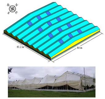 | Model TG Number of spans (n): 9 Width of span (m): 6.8 Total width (m): 61.2 Greenhouse length (m): 64 Surface area covered (Sac, m2): 3916.8 Rooftop ventilation area (m2): 134.4 Side ventilation area (m2): 128 Front ventilation area (m2):122.4 Total ventilation surface area (Tvsa, m2): 3848 Ventilation ratio (Tvsa/Sac, %): 10.17 Minimum height over gutter (m): 3.3 Minimum height above roof (m): 5.2 Maximum height over gutter (m): 6.1 Maximum height above roof (m): 8.0 |
| Greenhouse Schematic | Description |
|---|---|
 | Model MG Number of spans (n): 15 Width of span (m): 6.9 Total width (m): 103.5 Greenhouse length (m): 55 Surface area covered (Sac, m2): 5692.5 Rooftop ventilation area (m2): 313.5 Side ventilation area (m2): 220 Front ventilation area (m2): 414 Total ventilation surface area (sv, m2): 9475 Ventilation ratio (Tvsa/Sac, %): 16.64 Minimum height over gutter (m): 3.1 Minimum height above roof (m): 5.5 Maximum height over gutter (m): 5.4 Maximum height above roof (m): 8.2 |
| Greenhouse Schematic | Description |
|---|---|
 | Model HGT1 Number of spans (n): 24 Width of span (m): 6.8 Total width (m): 163.2 Greenhouse length (m): 60 Surface area covered (Sac, m2): 9656 Rooftop ventilation area (m2): 1507.2 Side ventilation area (m2): 228 Front ventilation area (m2): 620.16 Total ventilation surface area (Tvsa, m2): 2355.36 Ventilation ratio (Tvsa/Sac, %): 24.39 Minimum height over gutter (m): 3.0 Minimum height above roof (m): 5.2 Maximum height over gutter (m): 5.2 Maximum height above roof (m): 7.4 |
| Greenhouse Schematic | Description |
|---|---|
 | Model HGT2 Number of spans (n): 12 Width of span (m): 6.8 Total width (m): 81.6 Greenhouse length (m): 65.6 Surface area covered (Sac, m2): 5352.9 Rooftop ventilation area (m2): 942.72 Side ventilation area (m2): 236.16 Front ventilation area (m2): 293.76 Total ventilation surface area (Tvsa, m2): 1472.64 Ventilation ratio (Tvsa/Sac, %): 27.51 Minimum height over gutter (m): 3.0 Minimum height above roof (m): 5.4 Maximum height over gutter (m): 5.4 Maximum height above roof (m): 7.8 |
| Greenhouse Schematic | Description |
|---|---|
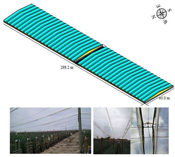 | Model SG Number of spans (n): 42 Width of span (m): 7.1 Total width (m): 298.2 Greenhouse length (m): 60 Surface area covered (Sac, m2): 17.892 Rooftop ventilation area (m2): 615 Side ventilation area (m2): 264 Front ventilation area (m2): 1312.1 Total ventilation surface area (Tvsa, m2): 2191.1 Ventilation ratio (Tvsa/Sac, %): 12.24 Minimum height over gutter (m): 3.5 Minimum height above roof (m): 5.5 Maximum height over gutter (m): 5.5 Maximum height above roof (m): 7.5 |
| Sensors Used Outside | Sensors Used Inside Greenhouses |
|---|---|
| 1 automatic weather station i-Metos Compact station (Pessl Instruments GmbH, Weiz, Austria). Data recording of temperature (°C), air humidity (%), wind speed (ms−1), direction (°), solar radiation (Wm−2) and precipitation (mm). 1 Autopilot Apcem 2 air CO2 concentration sensor (ppm) (Hydrofarm, China). | 40 type-T copper thermocouples (Copper/Constantan) used to measure temperature and relative humidity. 40 data recorder (Cox-Tracer Junior, Escort DLS, Edison, NJ, EE. UU.). 1 Autopilot Apcem 2 air CO2 concentration sensor (ppm) (Hydrofarm, China). 1 pyranometer Li-Cor LI-200SZ (LI-COR Inc, EE. UU.) |
| Greenhouse | Measurement Period |
|---|---|
| HGT1 | 1 February to 10 March. |
| HGT2 | 12 March to 22 April. |
| TG | 24 April to 30 May. |
| MG | 1 June to 9 July. |
| SG | 12 July to 22 August. |
| ESRL | ESRL 1 | ESRL 2 | ESRL 3 | ESRL 4 | ESRL 5 |
|---|---|---|---|---|---|
| Solar radiation level (Wm−2). | [0, 0] | [0.1–91.8] | [91.9–274.1] | [274.2–486.3] | [486.4–968.8] |
| Temperatura (°C) | Humedad Relativa (%) | VPD (kPa) | ||||||||||||||||||||
|---|---|---|---|---|---|---|---|---|---|---|---|---|---|---|---|---|---|---|---|---|---|---|
| GT | ESRL | Modelo | c0 | c1 (°C) | (c0/c1) (%) | a (m) | AIC | BIC | Modelo | c0 | c1 (%) | (c0/c1) (%) | a (m) | AIC | BIC | Modelo | c0 | c1 (kPa) | (c0/c1) (%) | a (m) | AIC | BIC |
| TG | 1 | Circular | 0.08 | 0.49 | 16.3 | 12.08 | 46.6 | 52.8 | Circular | 0.01 | 0.121 | 8.2 | 6.67 | 57.9 | 63.7 | Circular | 0.00 | 0.0005 | 0.0 | 6.6 | −213.4 | −207.6 |
| TG | 2 | Circular | 0.00 | 0.07 | 0.0 | 13.12 | 35.4 | 41.6 | Circular | 0.00 | 0.48 | 0.0 | 3.75 | 116.7 | 122.4 | Circular | 0.00 | 0.0002 | 0.0 | 5.0 | −140.0 | −134.3 |
| TG | 3 | Esférico | 0.07 | 0.38 | 18.4 | 69.54 | 44.8 | 51.1 | Circular | 0.00 | 15.12 | 0.0 | 7.21 | 196.8 | 202.9 | Circular | 0.00 | 0.007 | 0.0 | 7.2 | −66.2 | −60.1 |
| TG | 4 | Esférico | 0.00 | 1.13 | 0.0 | 19.58 | 108.5 | 114.9 | Circular | 0.00 | 14.24 | 0.0 | 7.26 | 194.7 | 200.9 | Circular | 0.00 | 0.0095 | 0.0 | 8.0 | −53.8 | −47.7 |
| TG | 5 | Circular | 0.37 | 2.90 | 12.7 | 64.18 | 122.1 | 128.2 | Circular | 6.59 | 29.69 | 22.1 | 6.62 | 199.3 | 205.4 | Circular | 0.00 | 0.0165 | 0.0 | 7.9 | −35.2 | −29.1 |
| MG | 1 | Circular | 0.02 | 0.13 | 15.3 | 9.97 | 125.1 | 131.6 | Circular | 0.0 | 7.7 | 0.0 | 12.9 | 168.9 | 174.9 | Circular | 0.0 | 0.001 | 0.0 | 12.9 | −115.5 | −109.5 |
| MG | 2 | Circular | 0.00 | 0.18 | 0.00 | 13.42 | 48.4 | 54.6 | Circular | 0.0 | 10.5 | 0.0 | 13.6 | 178.8 | 184.8 | Circular | 0.0 | 0.003 | 0.0 | 13.7 | −96.3 | −90.3 |
| MG | 3 | Circular | 0.06 | 0.34 | 17.6 | 9.45 | 94.7 | 101.7 | Circular | 1.7 | 20.5 | 8.3 | 9.56 | 232.0 | 238.2 | Circular | 0.001 | 0.028 | 3.5 | 9.7 | −41.3 | −35.1 |
| MG | 4 | Esférico | 0.11 | 0.59 | 18.6 | 9.88 | 99.4 | 105.9 | Circular | 0.0 | 65.7 | 0.0 | 12.6 | 253.5 | 259.7 | Circular | 0.0 | 0.033 | 0.0 | 12.5 | −12.2 | −5.9 |
| MG | 5 | Circular | 0.00 | 0.92 | 0.00 | 15.39 | 108.4 | 114.9 | Circular | 0.0 | 84.3 | 0.0 | 12.9 | 262.2 | 268.4 | Circular | 0.0 | 0.052 | 0.0 | 12.9 | 3.2 | 9.4 |
| SG | 1 | Circular | 0.02 | 0.16 | 15.3 | 9.83 | 125.1 | 54.9 | Circular | 2.8 | 14.1 | 20.1 | 9.97 | 166.7 | 172.0 | Circular | 0.00 | 0.002 | 0.0 | 11.5 | −101.8 | −95.8 |
| SG | 2 | Circular | 0.10 | 0.90 | 11.1 | 19.48 | 48.4 | 52.2 | Circular | 2.5 | 22.5 | 11.4 | 9.99 | 163.4 | 168.7 | Circular | 0.00 | 0.005 | 0.0 | 9.94 | −70.7 | −64.8 |
| SG | 3 | Circular | 0.00 | 0.52 | 0.0 | 20.40 | 94.7 | 88.3 | Circular | 6.9 | 38.7 | 18.0 | 9.82 | 194.3 | 199.8 | Circular | 0.00 | 0.034 | 0.0 | 9.85 | −5.8 | 0.3 |
| SG | 4 | Circular | 0.00 | 1.70 | 0.0 | 20.76 | 99.4 | 135.0 | Circular | 5.4 | 58.7 | 9.2 | 9.99 | 210.7 | 216.2 | Circular | 0.005 | 0.11 | 4.5 | 10.9 | 27.0 | 33.2 |
| SG | 5 | Circular | 0.00 | 3.10 | 0.0 | 20.65 | 147.7 | 154.1 | Circular | 0.0 | 114.1 | 0.0 | 10.8 | 227.6 | 233.1 | Circular | 0.0 | 0.22 | 0.0 | 12.9 | 53.1 | 59.4 |
| HGT1 | 1 | Gaussiano | 0.02 | 0.12 | 16.6 | 105.9 | 22.6 | 26.6 | Gaussiano | 0.00 | 0.00 | 0.0 | 3.54 | −20.47 | −17.6 | Circular | 0.0 | 0.0 | 0.0 | 35.94 | −137.4 | −134.4 |
| HGT1 | 2 | Gaussiano | 0.02 | 0.12 | 16.6 | 26.16 | 17.8 | 21.8 | Gaussiano | 0.05 | 0.23 | 21.7 | 22.6 | 12.66 | 15.7 | Gaussiano | 0.0 | 0.0 | 0.0 | 23.06 | −118.4 | −115.3 |
| HGT1 | 3 | Circular | 0.00 | 0.20 | 0.0 | 28.91 | 30.1 | 34.1 | Gaussiano | 0.07 | 0.41 | 17.1 | 3.44 | 39.31 | 42.4 | Circular | 0.0 | 0.0 | 0.0 | 13.44 | −81.3 | −78.0 |
| HGT1 | 4 | Circular | 0.08 | 0.53 | 15.1 | 26.40 | 53.3 | 57.2 | Gaussiano | 0.06 | 0.28 | 21.4 | 16.7 | 27.37 | 28.5 | Circular | 0.0 | 0.002 | 0.0 | 17.40 | −54.7 | −51.3 |
| HGT1 | 5 | Circular | 0.07 | 0.90 | 7.1 | 18.85 | 64.0 | 68.0 | Circular | 0.01 | 4.12 | 0.24 | 17.0 | 80.31 | 83.6 | Circular | 0.0001 | 0.003 | 3.3 | 17.85 | −41.1 | −37.8 |
| HGT2 | 1 | Gaussiano | 0.04 | 0.25 | 16.0 | 19.91 | 2.4 | 6.6 | Gaussiano | 0.0 | 0.001 | 0.0 | 8.34 | −50.8 | −47.2 | Circular | 0.0 | 0.0 | 0.0 | 14.09 | −203.2 | −199.6 |
| HGT2 | 2 | Circular | 0.0 | 0.053 | 0.0 | 14.09 | 5.9 | 9.7 | Circular | 0.0 | 0.046 | 0.0 | 14.09 | 3.5 | 7.1 | Circular | 1.88 | 0.0 | 0.0 | 14.09 | −143.2 | −139.5 |
| HGT2 | 3 | Circular | 0.0 | 0.115 | 0.0 | 14.09 | 21.4 | 25.4 | Circular | 0.0 | 0.645 | 0.0 | 14.09 | 51.1 | 54.7 | Circular | 0.0 | 0.0 | 0.0 | 14.09 | −85.5 | −81.95 |
| HGT2 | 4 | Circular | 0.0 | 0.344 | 0.0 | 14.09 | 43.4 | 47.4 | Circular | 0.0 | 2.268 | 0.0 | 14.09 | 77.4 | 81.2 | Circular | 0.0 | 0.002 | 0.0 | 14.09 | −61.0 | −57.3 |
| HGT2 | 5 | Circular | 0.0 | 0.67 | 0.0 | 14.09 | 56.7 | 60.7 | Circular | 0.0 | 5.048 | 0.0 | 14.09 | 92.6 | 96.4 | Circular | 0.0 | 0.005 | 0.0 | 14.09 | −40.2 | −36.7 |
Publisher’s Note: MDPI stays neutral with regard to jurisdictional claims in published maps and institutional affiliations. |
© 2022 by the authors. Licensee MDPI, Basel, Switzerland. This article is an open access article distributed under the terms and conditions of the Creative Commons Attribution (CC BY) license (https://creativecommons.org/licenses/by/4.0/).
Share and Cite
Villagrán, E.; Flores-Velazquez, J.; Akrami, M.; Bojacá, C. Microclimatic Evaluation of Five Types of Colombian Greenhouses Using Geostatistical Techniques. Sensors 2022, 22, 3925. https://doi.org/10.3390/s22103925
Villagrán E, Flores-Velazquez J, Akrami M, Bojacá C. Microclimatic Evaluation of Five Types of Colombian Greenhouses Using Geostatistical Techniques. Sensors. 2022; 22(10):3925. https://doi.org/10.3390/s22103925
Chicago/Turabian StyleVillagrán, Edwin, Jorge Flores-Velazquez, Mohammad Akrami, and Carlos Bojacá. 2022. "Microclimatic Evaluation of Five Types of Colombian Greenhouses Using Geostatistical Techniques" Sensors 22, no. 10: 3925. https://doi.org/10.3390/s22103925
APA StyleVillagrán, E., Flores-Velazquez, J., Akrami, M., & Bojacá, C. (2022). Microclimatic Evaluation of Five Types of Colombian Greenhouses Using Geostatistical Techniques. Sensors, 22(10), 3925. https://doi.org/10.3390/s22103925