Abstract
The urban spatial structure is a key feature of the distribution of social and economic resources. The spatial structure of an urban agglomeration is an abstract relationship expression of urbanization. Urban agglomerations develop for multiple reasons, including urban planning and natural evolution. To date, most research related to urban agglomeration has been based on single data source, which is a limitation. This research aims to propose a spatial structure identification method for urban agglomerations via a complex network based on nighttime light data and railway data. Firstly, we extracted the urban built-up area using defense meteorological satellite program/operational line scanner (DMSP/OLS) data, and divided it into urban objects to obtain the nighttime light urban network (NLUN) by borough. Secondly, we aggregated railway stations at municipal level using railway operation data to obtain the railway urban network (RUN). Following this, we established a composite urban network (CUN) consisting of the NLUN and the RUN based on the composite adjacency matrix. Finally, the Louvain algorithm and the comprehensive strength index (CSI) were used to detect the communities and central nodes of the CUN and obtain the urban agglomerations and core cities. The results show that urban agglomeration identification based on the CUN has the best accuracy, which is 5.72% and 15.94% higher than that of the NLUN and RUN, respectively. Core cities in the urban agglomeration identified by the CSI in the CUN are at least 3.04% higher than those in the single-source urban network. In addition, the distribution pattern of Chinese urban agglomerations in the study area is expressed as “three vertical”, and the development level of urban agglomeration shows an unbalanced trend.
1. Introduction
Urban agglomeration is defined as a huge, multicore and multilevel urban group developed around core mega-cities. It is generally composed of several large cities, with a number of smaller cities or towns providing supporting resources for the core city [1]. Urban agglomeration is an important concept in economic growth and plays a significant role in global economic circulation and human-nature interaction [2]. Since the 18th century, with the shift in economic centers, the world has experienced massive global urban agglomerations, such as those around London, Paris and other cities in northwest Europe, North America and the Asia-Pacific, including Japan [3]. Unlike developed countries (e.g., U.S., U.K., France), China has experienced rapid urban construction, and urban agglomeration in China continues to increase and develop. In recent years, rapid urbanization in China has created several large urban agglomerations, such as the Yangtze River Delta, the Pearl River Delta and Jing-Jin-Ji. The spatial structure of urban agglomeration can reflect the social and economic relationship between cities [4]. Therefore, due to the key role of urban agglomeration in Chinese regional economies, the effective identification of spatial structure features in urban agglomerations has become a hot topic. Relevant data of urban agglomeration spatial structure features can support decision making to optimize urban planning and development. To date, research on urban spatial structures has mainly focused on the analysis of distance between cities, the importance of core cities [5], such as urban agglomerations [6,7,8,9,10], and multicenter structure identification [11,12,13]. Compared with traditional spatial analysis methods, the complex network method has advantages, in that it can reveal the development of urban agglomeration spatial structure via the urban agglomeration resource distribution.
Spatial network data and remote sensing image data are popular sources for identifying the spatial structure of urban agglomeration. Because of their natural network properties, spatial network data (e.g., railway, road, logistics and social trajectory networks) are regarded as key data sources for research [14,15,16]. Additionally, considering the large-scale regional characteristics of the spatial structure of urban agglomeration, traffic network data such as railway and road network data are key sources for relevant research. Finally, nighttime light data have become a crucial data source in the spatial structure identification of urban agglomeration in recent years, e.g., DMSP/OLS and NPP/VIIRS data [17,18]. However, the development of urban agglomerations is also affected by other conditions (e.g., urban planning), which cannot be fully explained by a single data source. Composite complex networks can integrate information from multiple source networks, but this requires that the multiple source networks have the same nodes. The spatial network and the nighttime lighting network are different types of data that do not share the same nodes and therefore do not satisfy this requirement [19,20].
The complex network structure identification method for urban agglomeration can consider topology within spatial network data [21]. Urban agglomerations are identified by the community [22,23], and the core cities are mapped using a central node structure [24]. The community detection method can reveal the characteristics of relatively aggregated “groups” in a network, including Girvan-Newman [25], Louvain [26], fast-greedy [27], Walktrap [28], Infomap [29], label propagation [30] and fast unfolding [31]. The central node structure reflects the important node in a network, and its importance is measured by degree centrality, intermediate centrality, closeness centrality, fusion centrality, eigenvector centrality, Page Rank centrality, Topsis centrality, etc. [32]. Most current studies directly introduce topological structure-detection methods, without considering the geographical attributes of the urban agglomeration spatial structure. For example, the proximity relationship of nodes will be affected by spatial distance and present spatial non-stationarity, which will reduce the accuracy of central node structure detection.
In summary, a single data source cannot fully address the influence of natural and governmental factors in urban agglomeration identification. In addition, current methods based on complex network topology analysis do not pay sufficient attention to spatial attributes in urban agglomeration identification. Hence, this study proposes a method for the spatial structure identification of urban agglomeration based on multisource data and a complex network that can realize the division of urban agglomeration and the identification of core cities. The contributions of this study are summarized as follows: First, this study uses railway network data and nighttime light data to describe governmental factors and natural factors, respectively, and proposes a spatial structure analysis model for urban agglomeration, which considers multiple factors and provides a new approach for more accurate analysis of the urbanization process. Second, we design a composite network fusion method for multisource data, which provides a reliable method for multi-data fusion with different structures. Third, because the data source has spatial attributes, we propose a replication network-center-node structure-identification method considering spatial attributes, which improves recognition accuracy and makes a positive contribution to the application of complex network theory to spatial data analysis.
2. Data and Study Area
2.1. Study Area
The study area covered all cities in the eastern part of the Hu Line in mainland China, except for Hainan province, Taiwan province and Shennongjia Forestry District [33]. About 96 percent of the population and most urban agglomerations are located in this region. According to the 14th Five-Year Plan for National Economic and Social Development of the People’s Republic of China (The 14th Five-Year Plan), the region contains 15 national urban agglomerations, including Jing-Jin-Ji, Harbin-Changchun, Mid-southern Liaoning, Shandong Peninsula, Central Plain, Central Shanxi, Guanzhong Plain, the Yangtze River Delta, the middle reaches of the Yangtze River, the west coast of the Strait, Guangdong-Hong Kong-Macau Greater Bay Area, Beibu Gulf, Central Yunnan, Guizhou Plain and Cheng-Yu. These urban agglomerations contribute 85.53% of China’s GDP and are important drivers of China’s economic growth. The study area is shown in Figure 1.
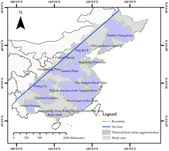
Figure 1.
The study area.
2.2. Data
The nighttime light data selected were the Defense Meteorological Satellite Program/Operational Line Scanner (DMSP/OLS) data from 2013. Unstable light sources, such as auroras and wildfires, as well as moonlight and clouds, were removed from the data. The Digital Number (DN) ranged from 0 to 63, and the spatial resolution was 30 arcsec. Passenger train data from 2014 were taken as the railway data. The railway data included train number, station, start and end time and running distance. This data totaled 2636 stations and 5036 train times, including local, fast, through and express trains.
2.3. Reference Data
2.3.1. Urban Agglomerations
This study takes the spatial scope of urban agglomerations in the 14th Five-Year Plan as its main basis, and the regional development level and existing research results as the auxiliary basis. We drew the reference urban agglomeration boundary as shown in Figure 2. The details included: (1) Inland areas with slow economic development, such as the Northeast and Southwest. According to relevant policy documents issued by the CPC Central Committee and the State Council, Liao-Ji-Hei and Yun-Gui were identified. (2) Areas with convenient water conservancy and transportation and rapid economic development in the middle reaches of the Yangtze River and the Yangtze River Delta. As indicated in the 14th Five-Year Plan, the urban agglomerations in the middle reaches of the Yangtze River and the Yangtze River Delta urban agglomeration are shown in Figure 3. These urban agglomerations develop along two axes and gradually divide into multiple single or multicore small urban agglomerations around the axes, such as Changsha-Nanchang, Wuhan Metropolitan, Hu-Su-Wan and Hangzhou-Ningbo. (3) In the highly developed areas of cities, the developed urban agglomerations merge the surrounding small ones. According to “The spatial development strategy planning of Taixin Integrated Economic Zone in central Shanxi urban agglomeration”, Jing-Jin-Ji should be built according to the Jing-Jin-Ji-Jin coordinated development guidance. (4) The urban agglomerations in regions with relatively stable economic development include Cheng-Yu, Guanzhong Plain, Shandong Peninsula, Central Plain, the west coast of the Strait, Beibu Gulf and the Guangdong-Hong Kong-Macau Greater Bay Area.
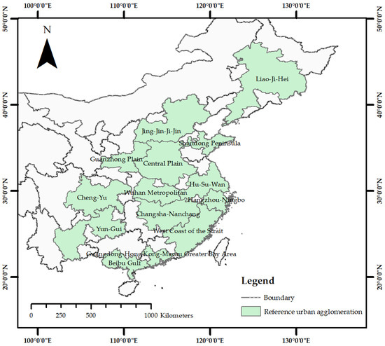
Figure 2.
The boundaries of reference urban agglomerations.
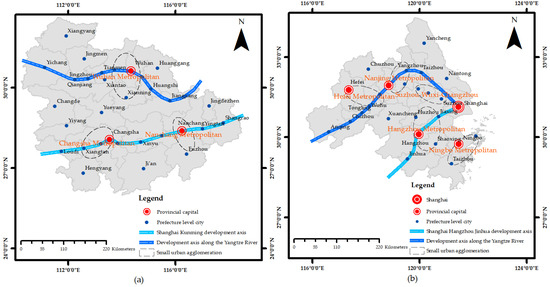
Figure 3.
Urban agglomeration planning map of the middle and lower reaches of the Yangtze River. (a) The middle reaches of the Yangtze River urban agglomeration; (b) The Yangtze River Delta urban agglomeration.
2.3.2. Core Cities
We defined the reference core cities according to the spatial scope and development plan of the reference urban agglomeration. There were 33 cities, and the relationship between reference urban agglomerations and core cities is shown in Table 1.

Table 1.
Reference urban agglomerations and core cities.
3. Method
This study proposes a method to identify the spatial structure of urban agglomerations based on multisource data and a complex network (Figure 4). Firstly, we used the threshold method to extract the built-up areas from the DMSP/OLS data. The built-up areas were divided into urban objects using administrative region boundaries, and the urban objects were regarded as nodes. The Gauss attenuation function was used to calculate the weight of the edge. The nighttime light urban network (NLUN) consisted of the nodes and edges obtained in the previous step. Secondly, all the train stations belonging to the same city were merged into one node, and the weight of the edge was calculated using distance and train frequency. The above nodes and edges formed the rail urban network (RUN). Thirdly, we constructed the nodes of the composite urban network (CUN) using spatial homogeneity, and fused the multi-type relationships using the composite adjacency matrix. Finally, the communities of the CUN detected using the Louvain algorithm were taken as the urban agglomeration, and the node with the highest comprehensive strength index (CSI) in each community was taken as the core city.
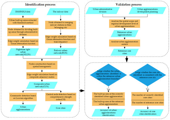
Figure 4.
Flowchart of the proposed spatial structure method for identification of urban agglomerations.
3.1. Preprocessing
The binary regression model was used to correct relative radiation for the DMSP/OLS data [34]. The study data were obtained by dividing the administrative region. The preprocessed DMSP/OLS data are shown in Figure 5.
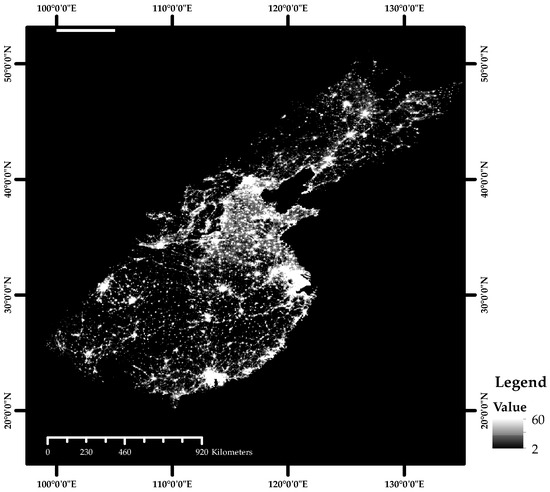
Figure 5.
Preprocessed DMSP/OLS Data.
The railway data included 2636 stations and 46,894 operational lines. We adjusted the data to obtain a city-node network. Railway stations in the same city were merged, the operational lines within the same city were removed, and the number of lines repeated between different cities were converted into frequency. The adjusted railway data had 269 nodes and 648 lines.
3.2. Composite Urban Network Construction
3.2.1. Nighttime Light Urban Network
Binary segmentation is a general method that was used to extract the built-up area from the DMSP/OLS data, and a region with or more was regarded as a built-up area [35]. Morphological expansion and corrosion algorithms optimized holes and profiles. If the ratio of the segmented edge built-up area to the built-up area of the administrative region was greater than 50%, the edge built-up area should be merged with the built-up area in the corresponding administrative region. is NLUN; stands for the set of city nodes, where is the total number of cities, is the set of edges, and is the adjacency matrix. The edges are the shortest lines between the polygon contours of the urban objects.
According to the first law of geography, closer objects are more connected [36]. The Gauss function is an attenuation function commonly used in gravity models, and is able to calculate the weight of the edges. The Gauss attenuation function is shown as:
where is the Euclidean distance between the nodes and , is a constant, and is the scale parameter.
3.2.2. Railway Urban Network
RUN is defined as , where is the set of edges and is the adjacency matrix. The node set is consistent with the NLUN. Combined with the Gauss attenuation function, we designed the edge-weight calculation method considering train frequency, which is shown as:
where is the frequency of trips, is a constant and is a scale parameter.
The scale parameter and control the distance attenuation amplitude. In order to ensure the consistency of the network, the density function of the normal distribution shows that 99.73% of the area is within the range of three standard deviations around the mean. The 13th Five-Year Plan for the development of modern integrated transport system points out that core cities and neighboring cities should be accessible within 2 h, which is referred to as the “two-hour access circle” (TAC) [37]. Based on the TAC and Equation (3), we can calculate the value of the scale parameters and :
where is the maximum access distance of TAC and is a constant.
3.2.3. Composite Urban Network Construction
Construction of the composite adjacency matrix is the key to obtaining a reasonable CUN, and the schematic diagram of CUN construction is shown in Figure 6. The CUN construction includes two cases. In the first case, there is only one connection type, and the original connection is retained. In the second case, there are multiple connection types, and a composite adjacency matrix is designed to integrate natural and governmental factors. The composite adjacency matrix is shown as:
where is the composite adjacency matrix, is a constant and is the single-layer network contribution degree. We calculate the modularity of the CUN at different , and determine according to the statistical law of modularity .
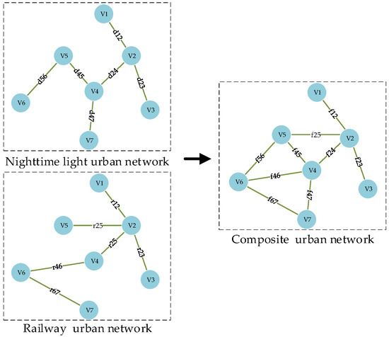
Figure 6.
Schematic diagram of composite urban network construction.
The binary valuation method is a commonly used method for approximating reasonable values to determine , and . Taking as an example, the initial range of is set at [0, 100]. When is set at 50, if the number of communities does not satisfy the requirement, we continue to set at 25 or 75 until the target number of communities is reached.
3.3. Spatial Structure Method to Identify Urban Agglomeration Using Composite Urban Network
We used the Louvain algorithm to detect communities. The algorithm is based on modularity [31], and its optimization goal is to maximize the modularity of the entire complex network. Degree centrality (DC) is the most direct measure of node centrality. The greater the DC of a node, the more important the node is. The DC is calculated as:
where denotes the number of edges connected to node and is the number of edges of node connected to all other nodes.
The DC focuses on the topological properties of the network, ignoring the weights of the edges and the nature of the nodes themselves. To solve this problem, we combine the natural conditions and governmental information relating to the nodes to construct a comprehensive strength index (CSI). The CSI provides the basis for central node detection. The larger the CSI, the more important the node, calculated as:
where denotes the centrality of weighted degree of the node , is the sum of the weights of the edges connected to the node , is the sum of the weights of all connected edges in the network, is the CSI of the node , is the built-up area of the node , is the number of stations of the node and and are normalized. The CSI of the nodes in each community structure are calculated separately. The node with the largest index is selected as the core city.
4. Results and Analysis
4.1. Composite Urban Network
The built-up area obtained by threshold segmentation was 388,514.75 km2. The municipal administrative region segmented the built-up area into 270 urban objects. The urban built-up area extraction results cover the major cities in the study area, and the urban objects are shown in Figure 7.
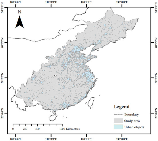
Figure 7.
The urban objects.
In the natural state, the TAC limits the connection distance of urban objects, which have a suitable relationship with the natural environment. The influences of highway construction and the natural environment are interactive [38] and the edge between urban objects can be approximated as a modern highway. According to the “Design Specification for Highway Alignment”, the modern highway running speed is generally 110 per hour [39] and urban objects that are more than 220 away are regarded as inaccessible. The scale parameter value of the NLUN was 73.33. The obtained NLUN included 270 nodes and 2520 edges. The NLUN is shown in Figure 8a.
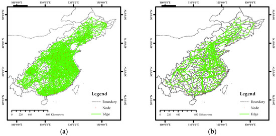
Figure 8.
Single-source urban network. (a) The nighttime light urban network; (b) The railway urban network.
Similarly, high-speed rail was used to calculate the TAC of the RUN. According to the “Code for Design of High-Speed Railway”, high-speed rail is defined as having a speed of 250 to 350 per hour. The average speed we chose for high-speed rail was 300 per hour. If two cities were more than 600 from each other, they were considered unreachable. The scale parameter value was 200. The final RUN consisted of 270 nodes and 628 edges, as shown in Figure 8b.
Equation (4) was used to construct the composite adjacency matrix, and was equally divided in a step of 0.1. The modularity of the CUN at different was calculated, and the corresponding relationship between modularity and single-layer network contribution is shown in Figure 9. When is 0.4, the modularity is the largest and the community detection result is the most effective. The CUN is shown in Figure 10. The number of edges was 2550, and the number of edges increased by 30 compared with the NLUN.
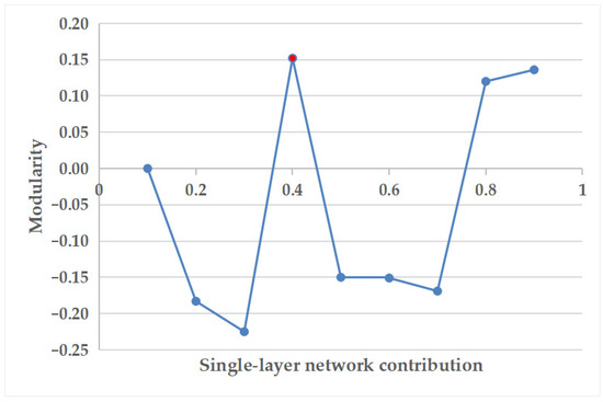
Figure 9.
Relationship between modularity and single-layer network contribution.
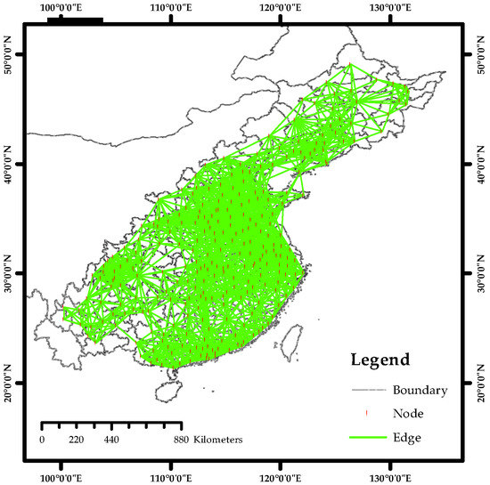
Figure 10.
The composite urban network.
4.2. Spatial Structure of Urban Agglomeration
4.2.1. Urban Agglomeration
The CUN, NLUN and RUN were all weighted networks, and their weight scales were inconsistent. First, the weights of the three urban networks were normalized. Following this, , and were obtained using the binary valuation method. When the number of communities was not less than 14 and not more than 15, , and were the best values. Finally, we used the Louvain algorithm to detect communities and map them to urban agglomerations. The urban agglomeration identification results are shown in Figure 11. The urban agglomeration of the NLUN was very similar to the CUN. All three urban networks had a central Anhui urban agglomeration and 14 urban agglomerations. The central Anhui urban agglomeration is about to develop, but it is small in scale and does not belong to the reference urban agglomeration.
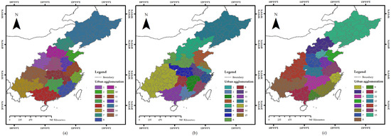
Figure 11.
The urban agglomeration identification results. (a) Nighttime light urban network; (b) Railway urban network; (c) Composite urban network.
The relationships between communities and urban agglomerations are shown in Table 2. Repeated communities in the table indicate that the community contains multiple reference urban agglomerations. Cities in the RUN region are more clearly constrained by regional planning. The division of urban agglomerations in more developed regions is more detailed, and the division of urban agglomerations in less developed regions is balanced and unified. Identification of urban agglomerations using the NLUN and CUN was more successful.
Table 2.
The relationships between communities and urban agglomerations.
We have used some experimental details to show the differences in the identification results for the three urban agglomerations. The urban agglomeration in the middle and lower reaches of the Yangtze River is shown in Figure 12a. The identification results from the RUN are broken, but their boundaries are basically the same as those of the reference data. The NLUN identification results are inconsistent with the reference data. The CUN achieved the best results, with the urban agglomeration boundaries combining the advantages of the abovementioned networks. The natural and economic conditions of the Pearl River Delta region are very close to those of the Beibu Gulf region in southern China. The CUN addresses the limitations of the NLUN, making it possible to effectively divide the Guangdong-Hong Kong-Macao Bay Area and the North Bay. The urban agglomeration in the southern region is shown in Figure 12b. Because of the strong agglomeration of railway lines in the southwest region, the RUNs here are integrated into a unified urban agglomeration. This result clearly does not correspond to the actual situation. The CUN weakens this effect. It is able to distinguish between Yunnan-Guizhou and Chengdu-Chongqing. The urban agglomeration in the Southwest is shown in Figure 12c. In general, the CUN improved on the single-source urban networks and achieved good results in identification of urban agglomerations and boundary extraction.
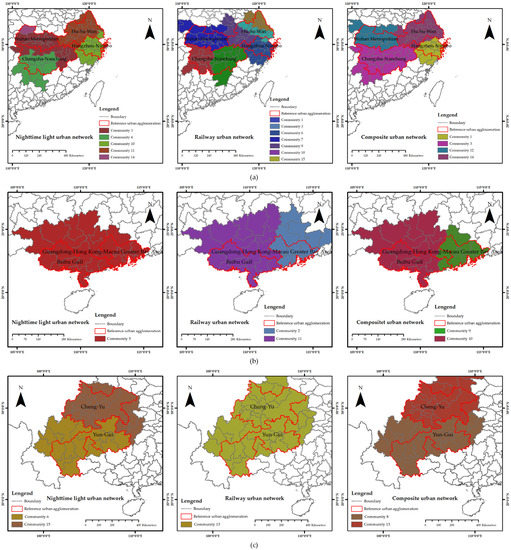
Figure 12.
Details of the urban agglomeration identification results. (a) The urban agglomeration in the middle and lower reaches of the Yangtze River; (b) The urban agglomeration in the southern region; (c) The urban agglomeration in the southwest region.
Based on the reference data, the identification results from the CUN, NLUN and RUN are analyzed here. The cities that fall within the boundaries of the reference data were classified correctly. Because the development levels of the various cities were different, the size of the built-up area could be used as a factor to measure the size of a city. We used the ratio of the built-up area of the correctly classified urban agglomeration to the built-up area of the reference urban agglomeration to determine the accuracy. The urban agglomeration identification accuracy is shown in Table 3. The CUN was 5.72% and 15.94% more accurate than the NLUN and the RUN, respectively. These results show that the CUN is more accurate than a single-source network. In addition, Figure 13 shows the comparison results between urban agglomeration extraction boundaries and reference urban agglomeration boundaries. In the figure, the built-up area is represented as a circle, and the larger the built-up area, the larger the size of the circle. Where the identification result overlaps with the reference result, this indicates a correct result for the region. An omission result for the region is indicated by the reference result without an identification result. However, the experimental data include most cities in China, some of which are not in the reference urban agglomeration. These cities belong to other identification results. As can be seen from Figure 13, the identification results from the CUN had the best agreement with the reference results, representing a significant improvement over the other two single-source networks.
Table 3.
Accuracy of urban agglomeration identification.
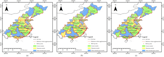
Figure 13.
Comparison results of urban agglomeration extraction boundaries and reference urban agglomeration boundaries. (a) Nighttime light urban network; (b) Railway urban network; (c) Composite urban network.
4.2.2. Core City Identification
The DC, weighted DC and CSI of the nodes in the NLUN, RUN and CUN were calculated. We used reference data to determine the number of core cities. If an urban agglomeration corresponded to multiple reference urban agglomerations, the sum of the core cities in the reference data was taken as the number of core cities. The core city identification results are shown in Figure 13. If the identified core city is the same as the core city from the reference data, the identification is correct. The core city identification results are shown in Table 4, and the accuracy is shown in Table 5.
Table 4.
Statistics of core city identification results.
Table 5.
Accuracy of Core Cities.
Based on the analysis in Figure 14 and Table 4 and Table 5, it can be seen that the accuracy of the core cities using CSI is significantly improved compared with that obtained by adopting degree or weighted degree centrality. Using CSI as the evaluation index, the core city identification of the CUN was 6.05% and 3.04% more accurate than the NLUN and RUN, respectively. The CUN and RUN were better than the NLUN at identifying core cities, such Nanchang, Hangzhou and Dalian. Some cities were incorrectly classified as core cities, mainly because they have larger built-up areas. For example, Weifang has a larger built-up area than Jinan.
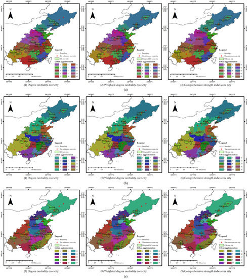
Figure 14.
The core city identification results. (a) Nighttime light urban network; (b) Railway urban network; (c) Composite urban network.
5. Discussion
This study proposes a spatial structure method for the identification of urban agglomerations based on multisource data, which can effectively identify urban agglomerations and core cities. Our method can visualize the spatial layout of urban agglomerations. It can be applied in the fields of urban agglomeration planning, urbanization analysis, regional economic organization and management, etc. We integrated the effects of natural and governmental factors by constructing a composite adjacency matrix. The comprehensive strength index integrates node connection strength, built-up area size and the number of railway stations to improve the accuracy of identification of core cities.
Although the approach described in this research has made some contributions, there are still some shortcomings to be addressed. First, we constructed the NLUN with urban objects as nodes and the distance between cities as the connection strength. The distance here is the minimum Euclidean distance between contour points of non-connected built-up areas. The accuracy of the contours determines the distance of the edge. Nighttime light data have a drawback. Large cities generally have a large number of uniformly distributed high-brightness pixels, whereas small cities have fewer and unevenly distributed high-brightness pixels. The result is that the threshold method cannot effectively identify the contours of the built-up area of small cities. This affects the reliability of the distances and has some impact on the structure of the NLUN.
Second, we analyzed the centrality of nodes based on their connectivity. Core cities were selected as those with the most centrality nodes. Coastal cities such as Hong Kong and Xiamen are limited by geography and cannot connect with more cities on land. These cities cannot be identified as core cities. This is clearly problematic. Finally, we used the Louvain algorithm to detect communities and took spatial autocorrelation into account in the adjacency matrix. However, whether spatial heterogeneity affects community detection is a key research topic for the future.
Third, there are a large number of methods for identifying the boundaries of urban agglomerations or built-up areas using remote sensing data and social sensing data [40,41]. These methods have the advantage of extracting urban features from different perspectives. However, researchers need to require massive social data, which is hard to acquire. Nighttime light data, which is an open access data, also can provide socio-economic information periodically [42]. We try to explore the structural features in this data, and apply it in the field of urban structure research. In addition, this research uses a weighted composite network to fuse nighttime lighting data and railway data. Although our method uses data fusion methods to improve the dimensionality of the information, it still needs to be upgraded in multisource data application.
Fourth, remote sensing technology has overstepped from natural resource information acquisition to socioeconomic information analysis [43], including applications such as GDP, population, electricity, carbon emissions, urbanization and poverty [44,45,46,47,48,49]. According to the law of spatial autocorrelation [50], the study used only distance to establish the intensity of urban connectivity. Although distance can effectively describe urban relationships from a spatial science perspective [18,51,52,53,54], it still does not achieve the information comprehensiveness of data such as artificial statistics and social perception data [55,56].
Finally, China’s urban agglomerations are mainly located east of the Hu Line, except for Lan-Xi, Hu-Bao-Er-Yu and the northern slope of the Tianshan Mountains. These three urban agglomerations can be abstracted to three separate network communities, respectively, and have less connection with eastern network communities. Thus, it is hard for us to establish a strong connection between cities on either side of the Hu Line using nighttime light data and railway data. There is uncertainty in the analysis of the proposed method for all Chinese cities, and we will keep our attention on this issue.
6. Conclusions
With the help of the theory related to complex networks, this study used 2013 DMSP/OLS data and 2014 railway operation data to construct the NLUN, RUN and CUN networks. Following this, we used the composite adjacency matrix to fuse the multisource data in order to identify urban agglomerations more accurately. The proposed CSI effectively describes the importance of city network nodes and provides a basis for identifying core cities. The urban agglomeration identification method using the CUN had the highest accuracy, with 5.72% and 15.94% improvements over methods using the NLUN and RUN, respectively. The CUN also had the highest accuracy in identifying core cities using CSI, which was at least 3.04% more accurate than the single-source urban networks.
In addition, we identified some urban agglomeration distribution characteristics. The regions with slower economic development are mainly limited by transportation and geographical conditions. This results in cities in these regions preferring to interact with cities within the same region rather than cities outside the region. The urban agglomerations in these areas have a high degree of convergence. In economically developed areas, cities have higher dynamics and urban agglomerations in these regions tend to fragment.
The urban agglomerations and core cities identified by the CUN show that the overall layout of urban agglomerations in China is “three vertical”. The urban agglomerations in the first vertical line include Guanzhong Plain, Chengyu and Yungui. The urban agglomerations in the second vertical line cover Jing-Jin-Ji-Jin, Central Plain, Wuhan Metropolitan, Changsha-Nanchang, Guangdong-Hong Kong-Macao Greater Bay Area and Beibu Gulf. Liao-Ji-Hei, Shandong Peninsula, Hu-Su-Wan, Hangzhou-Ningbo and the west coast of the Strait are urban agglomerations belonging to the third vertical line. The development levels of the urban agglomerations show an unbalanced trend.
Author Contributions
Conceptualization, Methodology, Z.X.; Writing, Original draft preparation, M.Y.; Reviewing and Editing, F.Z.; Investigation, M.C.; Software, M.T.; Supervision, L.S.; Data curation, G.S.; Visualization, R.L. All authors have read and agreed to the published version of the manuscript.
Funding
This research was supported in part by the National Natural Science Foundation of China under the grant 42101353, the Humanities and Social Sciences Foundation of the Ministry of Education of China (General Program) under the grant 21YJC790129 and the Basic Research Programs of Colleges and Universities of Liaoning Province of China under the grant LJKMZ20220946.
Data Availability Statement
The data that support the findings of this study are available from the corresponding author, (Fengyuan Zhang), upon reasonable request.
Conflicts of Interest
The authors declare that they have no known competing financial interests or personal relationships that could have appeared to influence the work reported in this article.
References
- Fang, C.; Yu, D. Urban agglomeration: An evolving concept of an emerging phenomenon. Landsc. Urban Plan. 2017, 162, 126–136. [Google Scholar] [CrossRef]
- Wu, J.; Weber, B.A.; Partridge, M.D. Rural-Urban Interdependence: A Framework Integrating Regional, Urban, and Environmental Economic Insights; Wiley: Hoboken, NJ, USA, 2017; pp. 464–480. [Google Scholar]
- Fang, C.; Wang, Z.; Ma, H. The theoretical cognition of the development law of China’s urban agglomeration and academic contribution. Acta Geogr. Sin 2018, 73, 651–665. [Google Scholar]
- Zhu, X.; Wang, Q.; Zhang, P.; Yu, Y.; Xie, L. Optimizing the spatial structure of urban agglomeration: Based on social network analysis. Qual. Quant. 2021, 55, 683–705. [Google Scholar] [CrossRef]
- Liu, X.; Huang, J.; Lai, J.; Zhang, J.; Senousi, A.M.; Zhao, P. Analysis of urban agglomeration structure through spatial network and mobile phone data. Trans. GIS 2021, 25, 1949–1969. [Google Scholar] [CrossRef]
- Zhang, Y.; Yang, D.; Zhang, X.; Dong, W.; Zhang, X. Regional structure and spatial morphology characteristics of oasis urban agglomeration in arid area—A case of urban agglomeration in northern slope of Tianshan Mountains, Northwest China. Chin. Geogr. Sci. 2009, 19, 341–348. [Google Scholar] [CrossRef]
- Yu, B.; Shu, S.; Liu, H.; Song, W.; Wu, J.; Wang, L.; Chen, Z. Object-based spatial cluster analysis of urban landscape pattern using nighttime light satellite images: A case study of China. Int. J. Geogr. Inf. Sci. 2014, 28, 2328–2355. [Google Scholar] [CrossRef]
- Skadins, T.; Krumins, J.; Berzins, M. Delineation of the boundary of an urban agglomeration: Evidence from Riga, Latvia. Probl. Rozw. Miast 2019, 62, 39–46. [Google Scholar] [CrossRef]
- Sudra, P. Spatial dispersion and the concentration of buildings in an urban agglomeration–a typology proposal for the Warsaw Metropolitan Area. Environ. Socio-Econ. Stud. 2020, 8, 81–96. [Google Scholar] [CrossRef]
- Tan, X.; Huang, B. Identifying Urban Agglomerations in China Based on Density–Density Correlation Functions. In Annals of the American Association of Geographers; Taylor & Francis: Abingdon, UK, 2022; pp. 1–19. [Google Scholar]
- He, X.; Cao, Y.; Zhou, C. Evaluation of polycentric spatial structure in the urban agglomeration of the pearl river delta (PRD) based on multi-source big data fusion. Remote Sens. 2021, 13, 3639. [Google Scholar] [CrossRef]
- Huang, Y.; Liao, R. Polycentric or monocentric, which kind of spatial structure is better for promoting the green economy? Evidence from Chinese urban agglomerations. Environ. Sci. Pollut. Res. 2021, 28, 57706–57722. [Google Scholar] [CrossRef]
- Ma, H.; Xu, X. Knowledge Polycentricity of China’s Urban Agglomerations. J. Urban Plan. Dev. 2022, 148, 04022014. [Google Scholar] [CrossRef]
- Su, X.; Zheng, C.; Yang, Y.; Yang, Y.; Zhao, W.; Yu, Y. Spatial Structure and Development Patterns of Urban Traffic Flow Network in Less Developed Areas: A Sustainable Development Perspective. Sustainability 2022, 14, 8095. [Google Scholar] [CrossRef]
- Zhang, P.; Zhao, Y.; Zhu, X.; Cai, Z.; Xu, J.; Shi, S. Spatial structure of urban agglomeration under the impact of high-speed railway construction: Based on the social network analysis. Sustain. Cities Soc. 2020, 62, 102404. [Google Scholar] [CrossRef]
- Fang, C.; Yu, X.; Zhang, X.; Fang, J.; Liu, H. Big data analysis on the spatial networks of urban agglomeration. Cities 2020, 102, 102735. [Google Scholar] [CrossRef]
- Peng, J.; Lin, H.; Chen, Y.; Blaschke, T.; Luo, L.; Xu, Z.; Hu, Y.n.; Zhao, M.; Wu, J. Spatiotemporal evolution of urban agglomerations in China during 2000–2012: A nighttime light approach. Landsc. Ecol. 2020, 35, 421–434. [Google Scholar] [CrossRef]
- Zheng, W.; Kuang, A.; Liu, Z.; Wang, X. Analysing the spatial structure of urban growth across the Yangtze River Middle reaches urban agglomeration in China using NPP-VIIRS night-time lights data. GeoJournal 2022, 87, 2753–2770. [Google Scholar] [CrossRef]
- Sun, X.; Wu, Y.; Feng, X. Structure Characteristics and Robustness Analysis of Multi-Layer Network of High Speed Railway and Ordinary Railway. J. Univ. Electron. Sci. Technol. China 2019, 2, 315–320. [Google Scholar]
- Bindu, P.; Thilagam, P.S.; Ahuja, D. Discovering suspicious behavior in multilayer social networks. Comput. Hum. Behav. 2017, 73, 568–582. [Google Scholar] [CrossRef]
- Millán, A.P.; Torres, J.J.; Bianconi, G. Complex network geometry and frustrated synchronization. Sci. Rep. 2018, 8, 1–10. [Google Scholar] [CrossRef]
- Hu, H.; Huang, X.; Li, P.; Zhao, P. Comparison of Network Structure Patterns of Urban Agglomerations in China from the Perspective of Space of Flows: Analysis based on Railway Schedule. J. Geo-Inf. Sci. 2022, 24, 1525–1540. [Google Scholar]
- Jian-bo, L.; Jing-hu, P. Spatial pattern of population flow among cities in China during the Spring Festival travel rush baed on “Tencent migration” data. Hum. Geogr. 2019, 34, 108–117. [Google Scholar]
- Wei, C.; Weidong, L.; Wenqian, K.; Nvying, W. The spatial structures and organization patterns of China’s city networks based on the highway passenger flows. Acta Geogr. Sin. 2017, 72, 224–241. [Google Scholar]
- Girvan, M.; Newman, M.E. Community structure in social and biological networks. Proc. Natl. Acad. Sci. USA 2002, 99, 7821–7826. [Google Scholar] [CrossRef] [PubMed]
- Zhang, Z.; Pu, P.; Han, D.; Tang, M. Self-adaptive Louvain algorithm: Fast and stable community detection algorithm based on the principle of small probability event. Phys. A Stat. Mech. Appl. 2018, 506, 975–986. [Google Scholar] [CrossRef]
- Clauset, A.; Newman, M.E.; Moore, C. Finding community structure in very large networks. Phys. Rev. E 2004, 70, 066111. [Google Scholar] [CrossRef]
- Raghavan, U.N.; Albert, R.; Kumara, S. Near linear time algorithm to detect community structures in large-scale networks. Phys. Rev. E 2007, 76, 036106. [Google Scholar] [CrossRef]
- Xueguang, M.; Yu, L. Spatial Structure and Connection of Cities in China Based on Air Passenger Transport Flow. Econ. Geogr. 2018, 38, 47–57. [Google Scholar]
- Lu, F.; Liu, K.; Duan, Y.; Cheng, S.; Du, F. Modeling the heterogeneous traffic correlations in urban road systems using traffic-enhanced community detection approach. Phys. A Stat. Mech. Appl. 2018, 501, 227–237. [Google Scholar] [CrossRef]
- Blondel, V.D.; Guillaume, J.-L.; Lambiotte, R.; Lefebvre, E. Fast unfolding of communities in large networks. J. Stat. Mech. Theory Exp. 2008, 2008, P10008. [Google Scholar] [CrossRef]
- Zhang, Q.; Yuan, T. Analysis of China’s Urban Network Structure from the Perspective of “Streaming”. In Proceedings of the 2018 26th International Conference on Geoinformatics, Kunming, China, 28–30 June 2018; pp. 1–7. [Google Scholar]
- Huanyong, H. Distribution of China’s population with statistical tables and density maps. Acta Geogr. Sin. 1935, 2, 33–74. [Google Scholar]
- Weng, Q. National Trends in Satellite-Observed Lighting: 1992–2012. In Global Urban Monitoring and Assessment through Earth Observation; CRC Press: Boca Raton, FL, USA, 2014; pp. 120–143. [Google Scholar]
- Ma, T.; Zhou, C.; Pei, T.; Haynie, S.; Fan, J. Quantitative estimation of urbanization dynamics using time series of DMSP/OLS nighttime light data: A comparative case study from China’s cities. Remote Sens. Environ. 2012, 124, 99–107. [Google Scholar] [CrossRef]
- GOYENA, R. A computer movie simulating urban growth in the detroit region. J. Chem. Inf. Model. 2019, 53, 1689–1699. [Google Scholar]
- Xiaoyue, Y. Study on 2-Hour Accessibility of High Speed Transportation Network in Yangtze River Delta City Group; Shanghai Normal University: Shanghai, China, 2021. [Google Scholar]
- Chao, L. Relationship between natural environment and highway engineering construction zoning. Public Commun. Sci. Technol. 2014, 6, 73+57. [Google Scholar]
- Xue-jun, W.; Yi-dong, Y.; Jing, F. Study on Expressway Operation Speed. J. Highw. Transp. Res. Dev. 2002, 19, 80–82. [Google Scholar]
- He, X.; Yuan, X.; Zhang, D.; Zhang, R.; Li, M.; Zhou, C. Delineation of urban agglomeration boundary based on multisource big data fusion—A case study of Guangdong–Hong Kong–Macao Greater Bay Area (GBA). Remote Sens. 2021, 13, 1801. [Google Scholar] [CrossRef]
- Cao, W.; Dong, L.; Wu, L.; Liu, Y. Quantifying urban areas with multi-source data based on percolation theory. Remote Sens. Environ. 2020, 241, 111730. [Google Scholar] [CrossRef]
- Gibson, J.; Olivia, S.; Boe-Gibson, G.; Li, C. Which night lights data should we use in economics, and where? J. Dev. Econ. 2021, 149, 102602. [Google Scholar] [CrossRef]
- Li, D.; Guo, W.; Chang, X.; Li, X. From earth observation to human observation: Geocomputation for social science. J. Geogr. Sci. 2020, 30, 233–250. [Google Scholar] [CrossRef]
- Shi, K.; Wu, Y.; Li, D.; Li, X. Population, GDP, and Carbon Emissions as Revealed by SNPP-VIIRS Nighttime Light Data in China with Different Scales. IEEE Geosci. Remote Sens. Lett. 2022, 19, 1–5. [Google Scholar] [CrossRef]
- Stokes, E.C.; Seto, K.C. Characterizing urban infrastructural transitions for the Sustainable Development Goals using multi-temporal land, population, and nighttime light data. Remote Sens. Environ. 2019, 234, 111430. [Google Scholar] [CrossRef]
- Hu, T.; Wang, T.; Yan, Q.; Chen, T.; Jin, S.; Hu, J. Modeling the spatiotemporal dynamics of global electric power consumption (1992–2019) by utilizing consistent nighttime light data from DMSP-OLS and NPP-VIIRS. Appl. Energy 2022, 322, 119473. [Google Scholar] [CrossRef]
- Chen, J.; Gao, M.; Cheng, S.; Liu, X.; Hou, W.; Song, M.; Li, D.; Fan, W. China’s city-level carbon emissions during 1992–2017 based on the inter-calibration of nighttime light data. Sci. Rep. 2021, 11, 1–13. [Google Scholar] [CrossRef] [PubMed]
- Chen, D.; Zhang, Y.; Yao, Y.; Hong, Y.; Guan, Q.; Tu, W. Exploring the spatial differentiation of urbanization on two sides of the Hu Huanyong Line—based on nighttime light data and cellular automata. Appl. Geogr. 2019, 112, 102081. [Google Scholar] [CrossRef]
- Yong, Z.; Li, K.; Xiong, J.; Cheng, W.; Wang, Z.; Sun, H.; Ye, C. Integrating DMSP-OLS and NPP-VIIRS Nighttime Light Data to Evaluate Poverty in Southwestern China. Remote Sens. 2022, 14, 600. [Google Scholar] [CrossRef]
- Expert, P.; Evans, T.S.; Blondel, V.D.; Lambiotte, R. Uncovering space-independent communities in spatial networks. Proc. Natl. Acad. Sci. USA 2011, 108, 7663–7668. [Google Scholar] [CrossRef]
- Wang, C.; Yu, B.; Chen, Z.; Liu, Y.; Song, W.; Li, X.; Yang, C.; Small, C.; Shu, S.; Wu, J. Evolution of urban spatial clusters in China: A graph-based method using nighttime light data. Ann. Am. Assoc. Geogr. 2022, 112, 56–77. [Google Scholar] [CrossRef]
- Guo, R.; Wu, T.; Liu, M.; Huang, M.; Stendardo, L.; Zhang, Y. The construction and optimization of ecological security pattern in the Harbin-Changchun urban agglomeration, China. Int. J. Environ. Res. Public Health 2019, 16, 1190. [Google Scholar] [CrossRef]
- Zhang, M.; Miao, W.; Yang, Y.; Peng, C.; Huang, Y. Spatial-Temporal Features of Wuhan Urban Agglomeration Regional Development Pattern—Based on DMSP/OLS Night Light Data. J. Build. Constr. Plan. Res. 2017, 5, 14. [Google Scholar] [CrossRef][Green Version]
- Zhang, Z.; Liu, Y. Spatial Expansion and Correlation of Urban Agglomeration in the Yellow River Basin Based on Multi-Source Nighttime Light Data. Sustainability 2022, 14, 9359. [Google Scholar] [CrossRef]
- Zhao, Y.; Zhang, G.; Zhao, H. Spatial network structures of urban agglomeration based on the improved Gravity Model: A case study in China’s two urban agglomerations. Complexity 2021, 2021, 6651444. [Google Scholar] [CrossRef]
- He, X.; Zhu, Y.; Chang, P.; Zhou, C. Using Tencent User Location Data to Modify Night-Time Light Data for Delineating Urban Agglomeration Boundaries. Front. Environ. Sci. 2022, 10, 860365. [Google Scholar] [CrossRef]


Disclaimer/Publisher’s Note: The statements, opinions and data contained in all publications are solely those of the individual author(s) and contributor(s) and not of MDPI and/or the editor(s). MDPI and/or the editor(s) disclaim responsibility for any injury to people or property resulting from any ideas, methods, instructions or products referred to in the content. |
© 2022 by the authors. Licensee MDPI, Basel, Switzerland. This article is an open access article distributed under the terms and conditions of the Creative Commons Attribution (CC BY) license (https://creativecommons.org/licenses/by/4.0/).