Abstract
Solar energy is the fastest-growing clean and sustainable energy source, outperforming other forms of energy generation. Usually, solar panels are low maintenance and do not require permanent service. However, plenty of problems can result in a production loss of up to ~20% since a failed panel will impact the generation of a whole array. High-quality and timely maintenance of the power plant will reduce the cost of its repair and, most importantly, increase the life of the power plant and the total generation of electricity. Manual monitoring of panels is costly and time-consuming on large solar plantations; moreover, solar plantations located distantly are more complicated for humans to access. This paper presents deep learning-based photovoltaics fault detection techniques using thermal images obtained from an unmanned aerial vehicle (UAV) equipped with infrared sensors. We implemented the three most accurate segmentation models to detect defective panels on large solar plantations. The models employed in this work are DeepLabV3+, Feature Pyramid Network (FPN) and U-Net with different encoder architectures. The obtained results revealed intersection over union (IoU) of 79%, 85%, 86%, and dice coefficients of 87%, 92%, 94% for DeepLabV3+, FPN, and U-Net, respectively. The implemented models showed efficient performance and proved effective to resolve these challenges.
1. Introduction
Scientists worldwide have paid close attention to developing power plants that use environmentally friendly “green” energy in recent years. Innovative technologies and the emergence of new materials [1] make it possible to build solar power plants designed for autonomous power supply of commercial and industrial buildings of different power consumption. However, to ensure long-term trouble-free operation, a reliable and straightforward method for assessing the quality of solar panels after installation is required. Megawatt-class solar plants consist of thousands of panels and may have different defective panels due to the possibility of improper handling and installation [2]. Different solar module defects like micro-cracks, hot spots, delamination, and panel deformation due to external influences can become the reason for energy production shortages [3]. Traditionally, the defects of solar panels are inspected by a team of employees, which is slow, expensive, and imprecise. To speed up the inspection process and increase its accuracy, several artificial intelligence (AI) techniques including machine learning and deep learning algorithms can possibly be adopted as automatic tools. Inspection of solar panels using UAVs or drones became the most effective among other methods [4]. The scanned panel images are collected and fit into the deep learning model to learn how to recognize defects on the solar panels. The trained algorithm will detect faults in solar panels and perform classification of defective and non-defective cells [5,6].
Over the last few decades, the development of unmanned aircraft and the emergence of integrated aerial measurement systems [7] have made it possible to speed up data acquisition to analyze solar panels’ performance. The existing neural network solutions with possible algorithms in real time are usually the detection and segmentation of panels on solar plant systems. Semantic segmentation is an essential and exciting task in Computer Vision [8]. The segmentation problem is solved in projects such as autonomous driving systems [9], tracing a person’s figure on security cameras, and detecting and segmenting cancerous cells in the human body [10]. Before the era of deep learning, various algorithms for image processing techniques such as the threshold segmentation method [11], edge detection techniques [12], or graph-cut-based approach [13] were used for segmentation and depending on the area of interest to extract objects from the image. These methods are normally not suitable for complex images, resulting in a low-quality image. The growing popularity of deep learning approaches like neural networks can be applied to complex imaging systems for getting high-accuracy results. Deep learning-based image segmentation models have proved their remarkable performance, achieving the best accuracy rates on popular benchmark datasets. Most neural network algorithms for semantic segmentation have an architecture similar to FCN [14]. FCN is one of the first successful neural network architectures developed for the pixel-wise semantic segmentation of images. Various pre-trained convolutional networks, such as VGG [15] or ResNet [16], are often used as encoder networks. The U-net model [17] uses the idea of skip connections to store spatial information. The DeepLabV architecture [18] introduced three innovations: convolution with upsampled filters (atrous convolution, dilated convolution), spatial pyramidal pooling (ASPP), combining deep convolutional neural networks with probabilistic graphical models (CRF).
In general, the segmentation algorithms trained to detect solar panel defects would not be 100% accurate. As a result, some solar panels may be incorrectly classified as defective. The visual inspection methods can show efficiency changes in the solar station’s output, including thermal imaging diagnostics and electroluminescence inspection [19]. Electroluminescence (EL) of solar panels is one of the foremost modern approaches for diagnosing and testing solar panels’ imaging. Wuqin Tang et al. [20] proposed a framework for the automatic classification system of defective PV modules based on deep learning and demonstrated the PV panel micro-crack, finger interruption, and break. Sergiu Deitsch et al. [21] introduced a general framework to detect defective solar panel cells. They built a classifier pipeline of different solar cell defects based on SVM and CNN, where average accuracy rates are 82.44% and 88.42%, respectively. The inspection of solar panels using thermal infrared images can quickly identify faulty components of solar panels. Recently, a diagnosis system was developed to observe if hotspots were present in the image of solar panels using infrared (IR) imaging [22]. Another research [23] studied solar panels’ electricity production loss due to dirt, soiling, or bird dejections, in which they proposed thermographic non-destructive tests backed up with AI techniques to classify abnormal operating conditions, which led to a significant loss in solar panel efficiency. M. Waqar Akram et al. [24] conducted experiments on indoor and outdoor thermographic images for normal and defective PV modules. Moreover, they applied different image processing techniques such as edge detection, filtering, and color quantization to segment the edges of defected regions. One distinguishable research work on classifying defective solar panels is the fuzzy rule-based classification system [25]. Rather than focusing on hot spot objection, the primary purpose of this work is to classify progressive defects such as discoloring and delamination of solar panels. Their proposed classifier system gives a classification accuracy increase of 10% on average.
From the survey of the related works, we have concluded that most of the works related to defect detection are not reliable for inspections of big solar plants. They are primarily focused on details of solar cells and the classification of occurring problems. Meanwhile, our research’s main advantage is identifying the exact location of defected cells on the performance of the segmentation task. Our research work is focusing on the detection of faults in solar power plants from a high view and processing it with deep convolution segmentation techniques.
Based on above works, by using multiple deep learning models, the chance of misclassification is minimal. It is realized that the implementation of various segmentation models including U-Net, U-Net++, DeepLabV3, DeeplabV3+, PSPNet, and FPN should be adopted in solar panels’ imaging. Further, we tried different configurations and backbones to analyze their performance and impact on the accuracy of the models. Finally, three segmentation models with the highest performance on the test dataset were selected. We implemented three state-of-the-art segmentation models using DNN, including FPN [26], U-Net [17], and DeepLabV3+ [27] models. To compare accuracy results, we used different encoders for these three models, such as ResNet [16], EfficientNet [28], ResNext [29], and MobileNet [30]. After completing all experiments, we achieved the highest accuracy in terms of IoU score using the U-Net segmentation model. We should also mention that Efficientnet-b3 performed the best among other backbones.
2. Materials and Methods
2.1. Dataset
One of the datasets used in this paper is the open novel PV plant thermal l images dataset (http://vrai.dii.univpm.it/content/photovoltaic-thermal-images-dataset, accessed on 4 June 2021). The main difference from other related works is its application to large-scale plantations. Researchers used solar panel images before, but those datasets are either electroluminescence or thermal images captured from close views where the inspection is impossible on extensive solar plantations. A photovoltaic thermal image dataset contains multiple and single damaged cells in images. The dataset contains defective cells collected on a 66 MW power PV plant in Tombourke, South Africa. The images were captured during PV inspection with a clear sky and maximum irradiation from 21 to 27 January 2019. The advantage of this dataset over other similar research is that data acquisition occurred during the inspection of the PV plants. Therefore, the PV plant thermal dataset can be applied on a large-scale solar module plantation, reducing cost and time and being helpful for operators.
Accurate segmentation of defected cells in images is an essential task in analyzing the performance of solar power plants during an inspection. However, most of the time, datasets with an insufficient number of labeled images result in overfitting the training set [31]. To deal with this issue, we decided to increase the number of training samples by merging a newly acquired solar plant dataset—ours—with the existing thermal images dataset mentioned above and utilized in this research work [32]. Furthermore, by combining the datasets, we diversified image features such as the angle of the taken image, the drone’s height, image contrast, etc. As a result, the performance was higher than applying only one dataset. The newly acquired dataset was collected during the inspection of solar modules in New Jersey with the help of a specialized drone photography company [33]. To the best of our knowledge, the collected dataset used for photovoltaic plant fault detection is unique compared to existing works. For further information about the utilized dataset and tools for its collection, refer to Table 1 and Table 2, and Figure 1.

Table 1.
UAV and thermal camera specification.
Table 2.
Photovoltaic thermal image dataset (Combined).
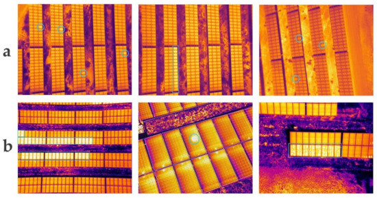
Figure 1.
Examples of raw images of both datasets, the blue circles and squares show the defective cells on the image. The thermal camera attached to the drone located the issue during a maintenance inspection. Sample images of thermal image dataset. (a) Photovoltaic thermal image dataset (existing); (b) our dataset (newly acquired).
To further increase the training dataset and improve the accuracy of semantic segmentation, we have utilized an augmentation technique called Albumentation [34]. It offers native support for the augmentation of images and masks together and covers the most use cases for image segmentation. This library is already widely adopted in the machine learning industry and much faster than torchvision. Therefore, we used this library instead of the original torchvision augmentation methods.
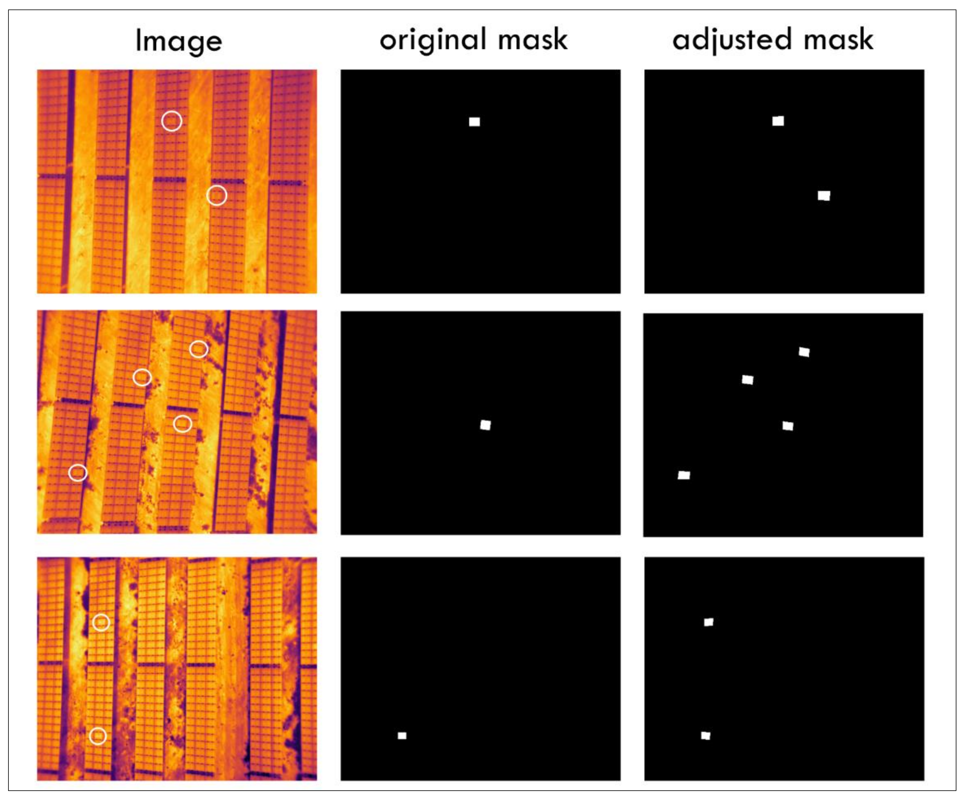
Thermal images associate a thermal value to each pixel. Hence, each image contains one or more defective cells annotated by the operator in this dataset. The obtained dataset was firstly used in this work [32] and received good results. However, after a thorough inspection, we identified label errors in this dataset. We discovered “defected” panels in some images not annotated into the mask. Nevertheless, the same panels are classified as “defected” from another view and angle in the other images. For a detailed view, refer to Figure 2. After calculation, we estimated at least 10% of errors in this dataset. This research [35] also explains that AI benchmark test datasets such as ImageNet, MNIST, and CIFAR have label errors and average at least 3.3%.
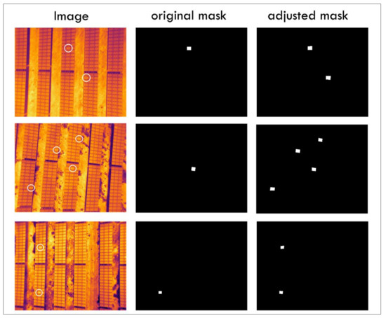
Figure 2.
Example mask images of incorrect annotation, the white circles and squares show the defective cells on the image. About 10% of the dataset has incorrectly annotated image masks.
In the case of misclassified solar panels, additional annotation of those images is essential to resolve this dataset problem. For this, we have used the open annotation tool LabelMe [36].
2.2. Photovoltaics Plant Faults Segmentation Using Deep Learning
Semantic segmentation means assigning a specific label to each pixel of the image. The main target is to locate objects and boundaries (lines, curvatures). This section mainly focused on deep learning-based semantic segmentation models with many objects of the same class as a single entity. Diverse deep learning-based segmentation models are designed by using the following configurations and hyperparameters specifications, as summarized in Table 3. We implemented different deep learning models and compared the results. FPN, U-Net, and DeepLabv3+ networks showed the highest dice scores among them. Feature Pyramid Network was the first model implemented using the solar plant dataset. FPN uses the pyramid form of CNN hierarchical features, generating feature pyramids with reliable semantic information at all levels. The FPN framework has a top-down structure and a horizontal connection to integrate shallow, high-resolution, and deep layers with rich semantic information. Thus, it is possible to quickly build a feature pyramid with reliable semantic information at all scales from a single input image on a single scale without a high cost. Another deep learning model used in this research is U-Net. Compared to the FPN structure, U-net follows the encoder–decoder architecture. The encoder gradually reduces spatial dimension by combining layers, and the decoder restores the object details and spatial dimension. There are also fast encoder-to-decoder connections to help the decoder better recover object details. The U-Net architecture can handle small objects in image segmentation tasks and achieve high accuracy using small datasets [37]. Optimizer “Adam” was utilized in all three deep learning models because of the faster computation time, and also required fewer parameters for the model tuning. For the activation function, we used “sigmoid”. This function exists in the range of 0 and 1. In this work, we must predict if the pixels in the predicted image belong to the object of interest (1) or background (0). Thus, the sigmoid function is the right choice. We used the specific values of data mean and standard deviation normalization because of ImageNet. As described in Table 3, we have implemented transfer learning, and ImageNet has its specific mean and standard deviation values. The final model implemented on the solar plant thermal image dataset is DeepLabV3+, using ResNet50 as a backbone. DeepLabV3+ uses only a Deep Convolution Neural Network with atrous convolution, following a spatial pooling process. The content of the following subset is about the semantic segmentation models implemented using PV thermal image dataset.
Table 3.
Configuration and hyperparameters specifications of implemented models.
2.2.1. FPN
FPN consists of bottom-up and top-down pathways. The bottom-up path is the process of convolutional computation. The spatial dimension of the feature map gets smaller by 1/2 as it shifts up. The features retrieved each time are the output of the last layer of each stage (the last layer has the most vital semantic feature), forming a feature pyramid. We used ResNet50 as an encoder of feature maps. It utilizes the features of the last residual structure of each stage to activate the output. We defined these outputs as {C2, C3, C4, C5} corresponding to the outputs of conv2, conv3, conv4, and conv5, they have {4, 8, 16, 32} pixel pitches relative to the input image, as shown in Figure 3.
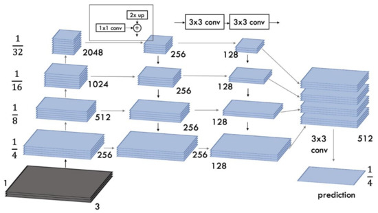
Figure 3.
Framework of FPN architecture for semantic segmentation.
The top-down path is done by upsampling the network, and the horizontal joint must combine the upsampling result with a feature map of the same size generated from the bottom-up pathway. Top-down feature maps undergo 1 × 1 convolution to reduce the channel size, and the feature maps of the ascending and descending paths are combined by elementwise addition. Subsequently, a 3 × 3 convolution is applied to each merged map to generate the final feature map layers for object segmentation, reducing the effect of aliasing when upsampled. This last set of feature maps is called {P2, P3, P4, P5}, corresponding to {C2, C3, C4, C5}, which have the exact spatial dimensions, respectively. Since all pyramid levels use joint classifiers/regressors, as in a traditional image pyramid with features, the feature size in the output d is fixed at d = 128, as illustrated in Figure 3. Thus, all additional convolutional layers have 128-channel outputs.
Since all the levels of P modules are rich in semantic features and have 128 channels each, they can be combined to produce the final segmented image. Hence, we have an absolute module with 512 channels. Finally, we applied a 3 × 3 convolution filter, batch normalization [38], and ReLU [39] activation in the final stage. Following this, we utilized spatial dropout and then upsampled output to the original image to regularize strongly correlated features and make the training computation more efficient.
2.2.2. U-Net
The U-net network does not have fully connected layers. It only uses each convolution part, i.e., the segmentation feature contains only pixels. For high-quality segmentation, U-net increases the amount of data by deforming images. The U-Net consists of a contracting path (downsampling) and an expansive path (upsampling). The downsampling part corresponds to typical convolutional network architecture. It repeatedly applies two 3 × 3 convolutions, followed by the ReLU activation function; then comes the max-pooling layer with a 2 × 2 filter. This process repeats in 4 steps and afterward comes a horizontal block of two 3 × 3 convolutions with ReLU activation, as shown in Figure 4. At each downsampling step, the number of feature channels is doubled. The upsampling path consists of 4 steps, too, known as the decoder part. It contains two 3 × 3 convolution layers, followed by 2 × 2 upsampling, which halves the number of feature channels. Finally, a 1 × 1 size convolution is used on the last layer to display each 64-channel feature map into the required number of classes. The general U-net architecture framework is demonstrated in Figure 4. The images are normalized and pre-processed before fitting the dataset into the model.
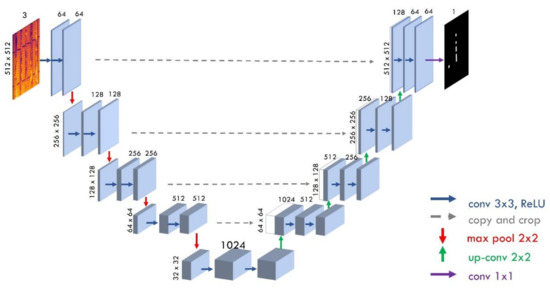
Figure 4.
Framework of U-Net architecture for semantic segmentation.
The shape of the input images is (N; 3; H; W), where N is the number of images, H and W define the height and weight of the images, respectively. The architecture utilizes pixel-wise softmax to the final feature map to obtain a predicted segmentation mask.
The formula of pixel-wise softmax can be defined as:
The pixel-wise softmax is a bit different compared to the original one. If we think of the output feature map as an image, each pixel is represented as K values, where K is the number of classes of interest. is the activation in feature channel k at pixel position x.
The loss function used in the training of U-Net is cross-entropy loss:
Here, the weighting (w) was added to the typical cross-entropy loss function to provide weighting to some pixels that are more critical than others.
The weight map is pre-processed using a morphological technique to the ground-truth segmentation mask. Its primary purpose is to identify thin borders between normal and defective panels. The weight map formula is given as:
Here, the is the distance to the nearest panel boundary at position x, while is the distance to the second closest panel boundary. Thus, the weight is much higher than in the image at the boundary. Overall, the purpose of using the weight map is to help the model learn the small separation borders between normal and defective panels.
The overall framework can be observed in Figure 4.
2.2.3. DeepLabV3+
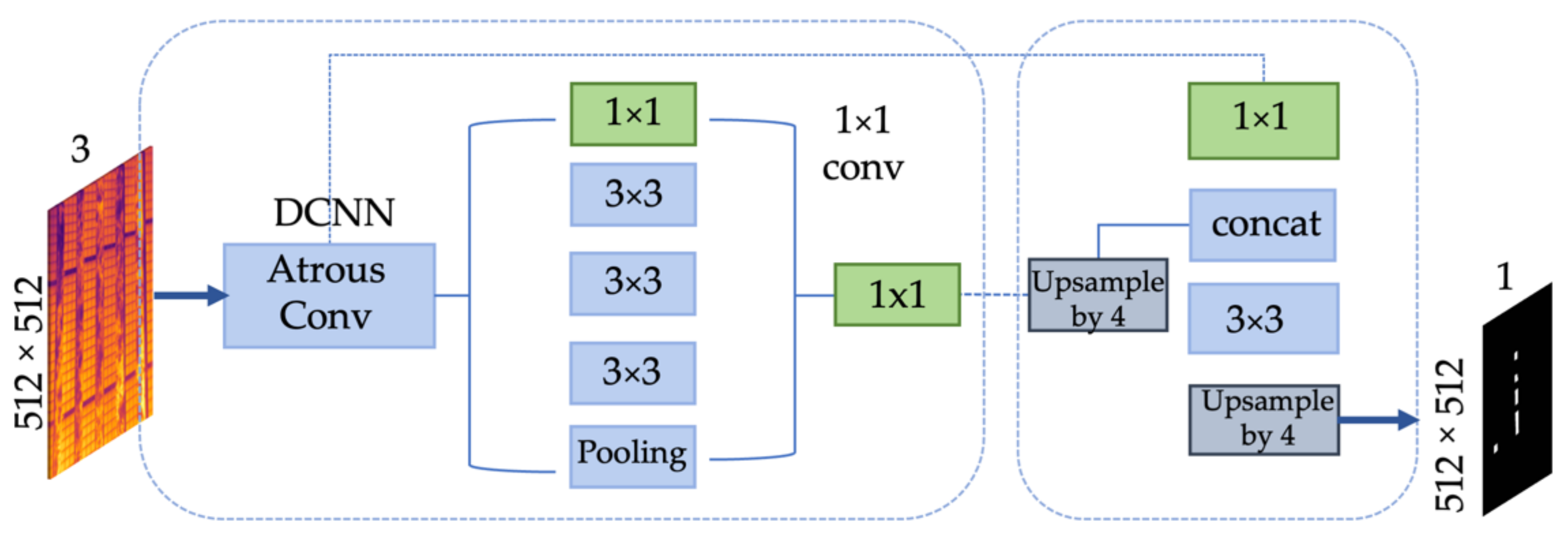
Spatial pyramid pooling, like the encoder–decoder architecture, is used in deep neural networks for semantic segmentation tasks. The spatial pyramid pooling can encode contextual information at different scales by transforming input features through filters or downscaling layers with different parameters. On the other hand, the encoder–decoder technique processes clear boundaries of objects by successive restoration of spatial information. The model DeepLabV3+ uses both approaches, adding a decoder to DeepLabv3 [40] to improve decoding accuracy, especially in object boundaries. The network input receives an image of 512 × 512 × 3. This image is fed to the input of the atrous convolution with the SPP module, as shown in Figure 5. Recall that the encoder can extract features with an arbitrary spatial resolution (the more, the better). The only limit here is the lack of computing power. In the previous DeepLabV3 architecture, the resolution of the output feature map of the encoder was 16 times less than the input. This output can be bilinearly scaled up to the original resolution, considered a primary decoder. However, such an implementation of the decoder may inaccurately reconstruct object boundaries. Therefore, a simple and relatively efficient decoder was proposed. The output of the encoder is first upsampled bilinearly by a factor of 4 and then connected to the corresponding low-level image features extracted by the encoder that has the exact spatial resolution. A 1 × 1 convolution is applied to these low-level features to reduce the number of channels, because corresponding features usually have many channels (256 or 512), which can outweigh the importance of high-level features and complicate the learning process. After concatenation, 3 × 3 convolution is applied to refine the features, followed by another simple bilinear upsampling by a factor of 4, as shown in Figure 5. In the DeepLabV3+ model, channel-by-channel separate convolution is used both in the atrous convolution with SPP module and in the decoder, which reduces the number of operations for calculating the layer output and thereby speeds up the image processing. Atrous convolutions are convolutional layers with extended filters, in which the areas between non-zero filter values are filled with zeros. In particular, for a one-dimensional signal, the output feature vector y with a one-dimensional input signal x and a filter w of length K looks like this:
where r is the degree of expansion, which determines the step when we select the input signal values. Note that for r = 1, atrous convolution is equivalent to ordinary convolution. This type of convolution increases the size of the kernel from k × k to , where r is essentially an adjustment parameter between local precision (small field of view) and image context assimilation (large field of view). Note that an increase in the output feature map of the encoder gives a significant increase in model performance but requires additional computation time (as described in [27]).
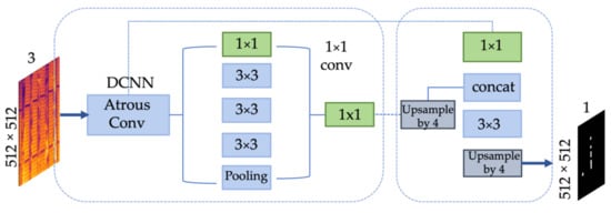
Figure 5.
Framework of DeepLabV3+ architecture.
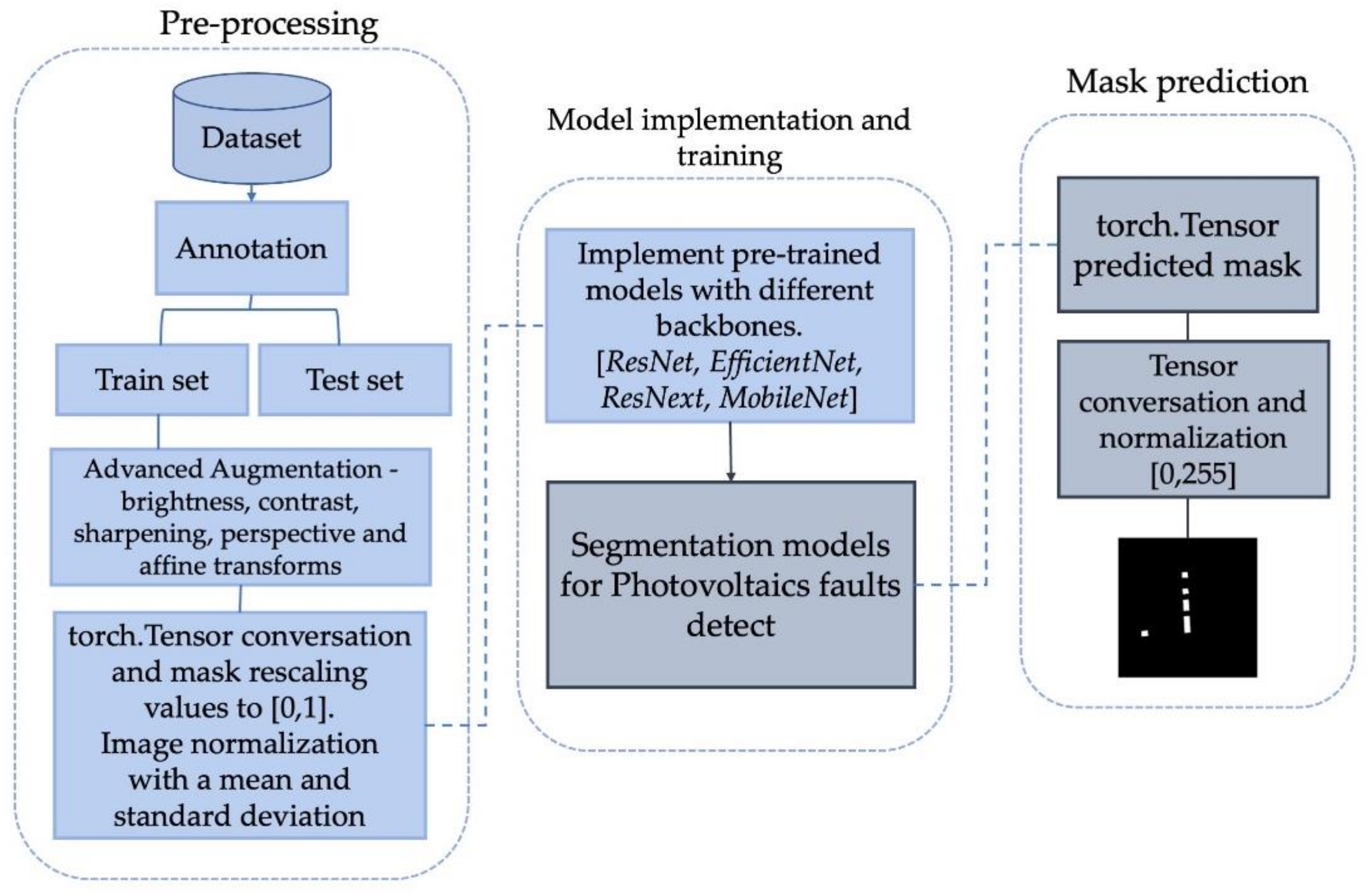
We discussed segmentation models trained using the solar panel fault dataset above. The overall workflow of the PV fault detection system is described in Figure 6. The details of the workflow framework follow.
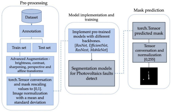
Figure 6.
A framework of Photovoltaics fault detection using deep learning.
The pre-processing stage required revising the existing dataset and found wrongly labeled masks around 10% by annotation process. Additionally, we have acquired a new dataset and combined it with the existing one for the PV fault detection. We have split the dataset into train and test subsets. Then, advanced augmentation methods are applied to further increase the number of training samples. These include change of brightness, contrast, sharpening, applied perspective, and affine transforms. Finally, RGB images were converted into torch tensors. They were normalized using standard deviation and mean values of ImageNet. The mask image values were rescaled to 0 and 1.
We have implemented three deep learning segmentation models with different backbones to compare the results. As an outcome, ResNet and EfficientNet backbones showed reasonably good accuracy (refer to Table 4). PV fault detection images went through all trained models to output the predicted mask at the testing phase. Next, the predicted tensors are converted into NumPy values and normalized to 0 and 255 for grayscale imaging, which are used as mask predictions.
Table 4.
PV plant faults detection and segmentation results with different encoders.
3. Results and Discussion
3.1. Performance Evaluation
This chapter visualized and described the experimenting results of deep learning segmentation models for the solar plant fault detection dataset. A common problem in image processing is detection or segmentation of a tiny anomalous region of a large image. In our case, segmentation is a binary mask, where the part of the defective solar panel is small, and the difference with regular panels is very little. This kind of data is often unbalanced. Quickly classified examples make up most of the training set and dominate the calculation of the loss function. We used the dice loss function to evaluate segmentation accuracy on the test set. It demonstrates the similarity or difference between the predicted result of the neural network and ground-truth indicators. Dice loss deals with the problem of the unbalanced dataset in terms of assessing the performance of segmentation [41]. The loss function can be expressed as:
where is ground-truth value and is predicted one.
The performance of the implemented segmentation models is evaluated by comparing ground-truth and prediction masks using Pixel Accuracy (PA), F1-score, Precision and Recall
Here, stands for the number of pixels belonging to class i, where it is predicted as class j. TP, TP, and FN represent True Positive, True Negative, and False Negative, respectively.
Due to class imbalance, where most of the pixels in the dataset belong to the background and a small part to the class of interest, the high accuracy of evaluation metrics applied above does not imply a good segmentation ability. To tackle this issue and calculate the performance of implemented models, we used an alternative metric called the Jaccard Index, also known as the IoU metric. It is determined as the ratio of overlap (intersection) and union area of A and B:
where is ground-truth and is predicted values. For more details, refer to Table 4.
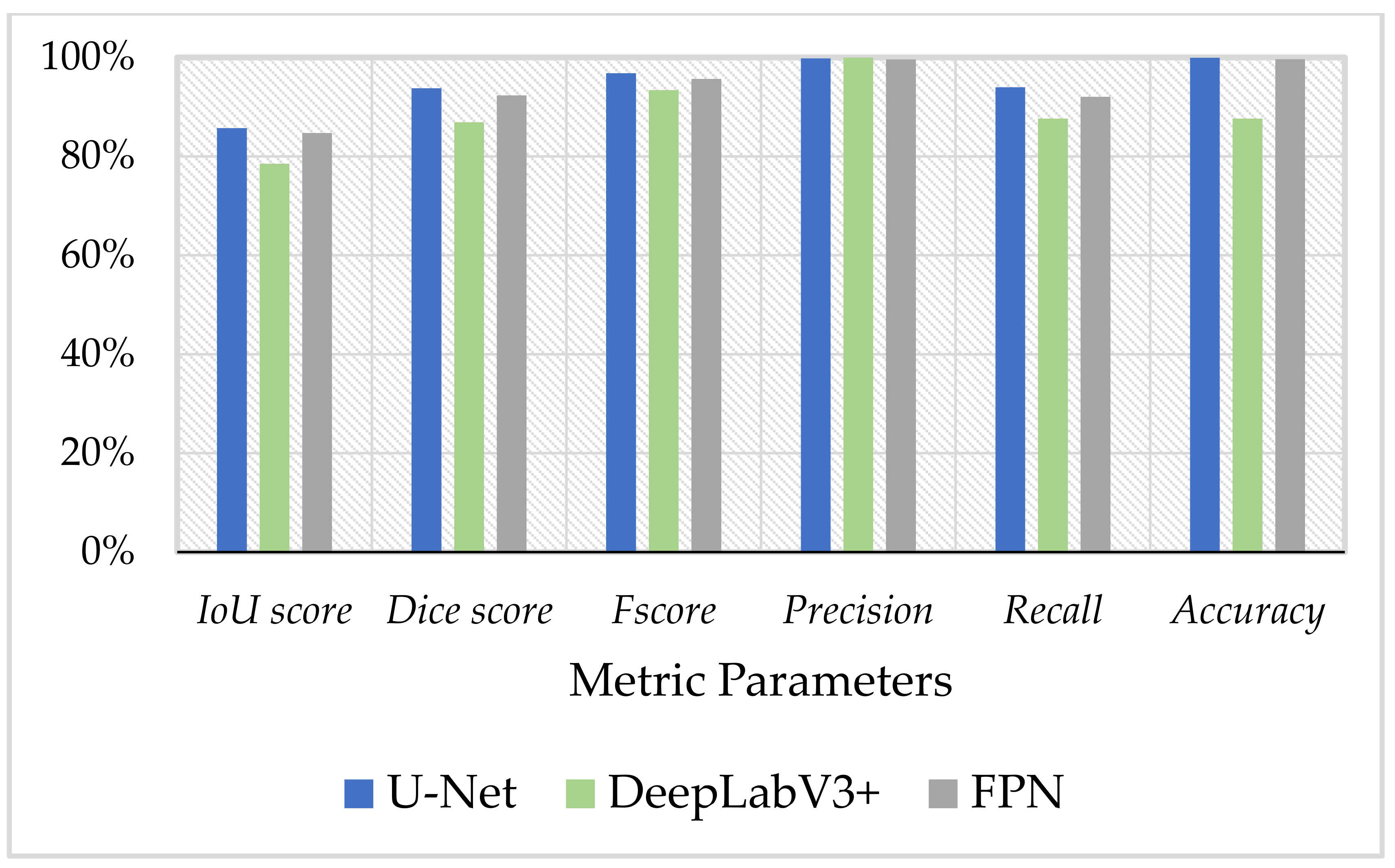
In this work, we evaluated three pre-trained deep learning models’ performance to test the solar plant fault detection images. As described in Table 4 and Figure 7, the U-Net model with a IoU score of 86% performed the best among other models; the following FPN could achieve a IoU score of 85%, and DeepLabV3 is 78%.
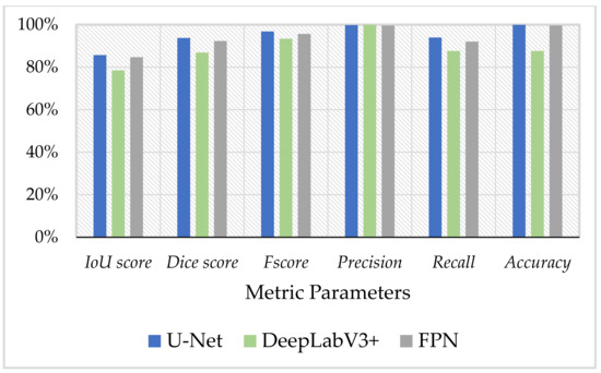
Figure 7.
Segmentation models’ performance evaluation results.
Figure 8 shows the training progress of segmentation models implemented in this work. We can observe some fluctuation during the first 30 epochs for the FPN model. U-Net and DeepLabV3+ models kept improving and decreasing the loss in calculations. In the end, the loss curve gradually decreases, proving that U-Net+ is more compatible with this work.
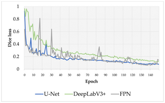
Figure 8.
Validation loss of three implemented models during the training process. The total number of epochs for training is 150.
3.2. Visualization Results of Solar Plant Fault Detection Experiments
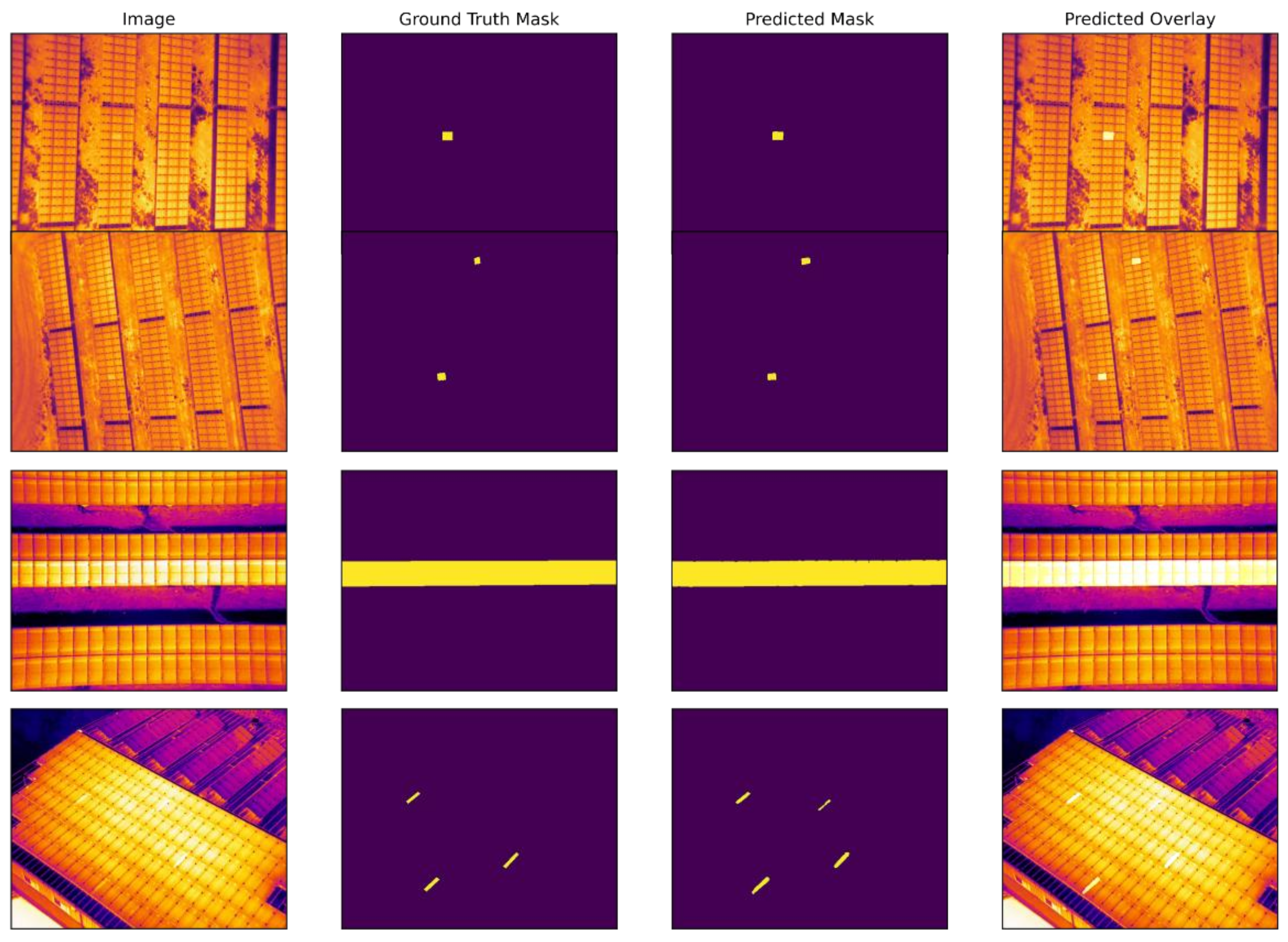
In this subsection, we discussed and visualized the experimental results of our three implemented segmentation models and compared them. The model results are visualized on images in the test set. As you can see in Figure 9, Figure 10 and Figure 11, the segmentation models show high-accuracy results in segmenting defective panels on solar plantations compared to traditional segmentation techniques. As shown in Figure 9, DeepLabV3+ provides relatively high segmentation efficiency. All the defective panels in the image were accurately identified, but there are errors (1–2%) in segmenting pixels as the object of interest in several images. However, in the last image of Figure 9, the predicted mask image is not well matched with the ground-truth mask image, which might result from a thresholding problem. Additionally, a weak contrast and high object brightness with the rest of the background may influence the accuracy of the prediction. Thus, it is important to conduct experiments using algorithms to improve image quality, contrast, and apply various filters in the future.
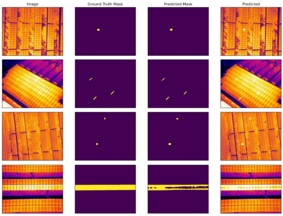
Figure 9.
Original, ground-truth mask, model-predicted mask and predicted overlay images of PV plant fault detection experiment using DeepLabV3+ segmentation model.

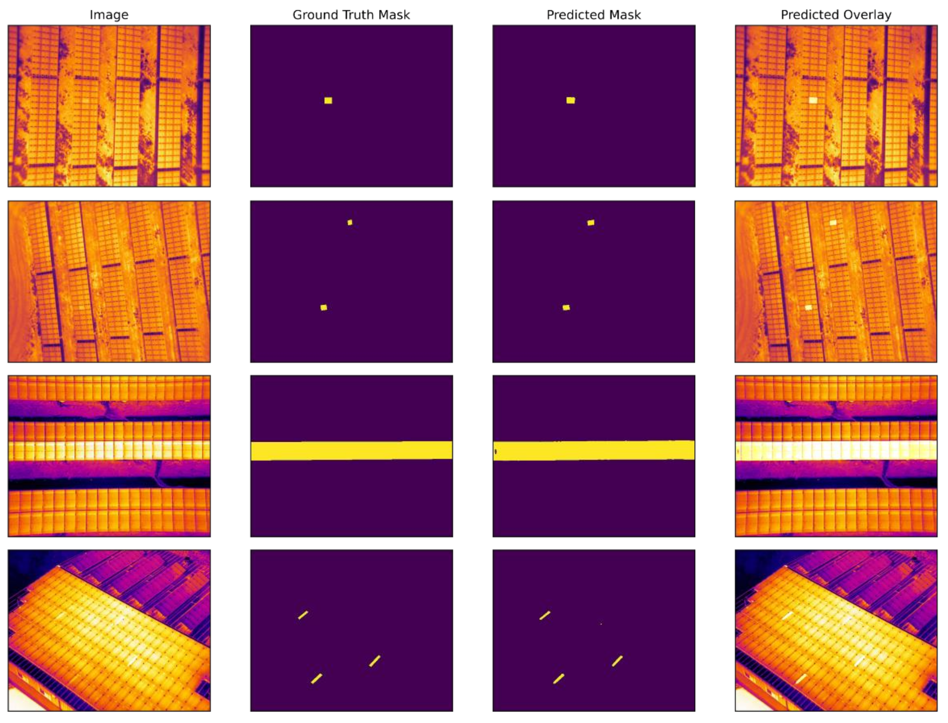
Figure 10.
Original, ground-truth mask, model-predicted mask and predicted overlay images of PV plant fault detection experiment using FPN segmentation model.
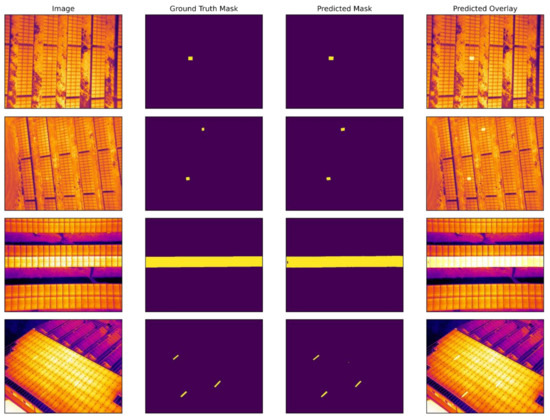
Figure 11.
Original, ground-truth mask, model-predicted mask and predicted overlay images of PV plant fault detection experiment using U-Net segmentation model.
The segmentation results using the FPN model are shown in Figure 10. The model performed efficiently in terms of detecting defective panels. We can observe the detection of one and a serial number of faulty solar panels, where two or more of the panels have been defected on the test dataset. However, you can note that the segmentation quality is not smooth when there are continuous or more than two defective solar panels in one image. There are two main reasons for this: an unbalanced training dataset and a relatively small number of pixels in the image belonging to the defective class.
Figure 11 shows the best result for U-Net. This neural network produces the cleanest masks without background and contours. FPN performs relatively close results, proved in the IoU and dice accuracy metrics. Both neural networks produce a smooth and accurate mask in test images.
4. Conclusions
This research work implemented standard approaches for semantic segmentation, such as FPN, U-Net, and DeepLabV3+ to detect defective panels on large-scale solar plantations. We have acquired a new dataset and combined it with the existing one for higher accuracy results. In order to choose the suitable algorithms, among various segmentation models, FPN, U-Net, and DeepLabv3+ networks showed the highest dice scores among them. The test experiments expressed the competitive results in semantic segmentation with a dice score of 0.94 (U-Net), 0.92 (FPN), and 0.87 (DeepLabV3+), resulting from the high accuracy of U-Net and FPN models. The obtained results revealed that deep learning-based segmentation models significantly outperform the traditional image segmentation approaches. Therefore, applying drones backed up with AI techniques can be valuable for operators in maintenance, error-fixing operations and lowering labor costs in manual processes.
Author Contributions
Conceptualization, S.J. and M.L.; methodology, S.J.; software, D.J.; validation, S.J., D.J. and M.L.; data curation, D.J. and S.J.; writing—original draft preparation, S.J.; writing—review and editing, D.J. and M.L.; supervision, M.L. All authors have read and agreed to the published version of the manuscript.
Funding
This research received no external funding.
Institutional Review Board Statement
Not relevant.
Informed Consent Statement
Not applicable.
Data Availability Statement
The data presented in this study are available on request from the corresponding author.
Acknowledgments
This work was supported by the “Human Resources Program in Energy Technology” of the Korea Institute of Energy Technology Evaluation and Planning (KETEP), granted financial resource from the Ministry of Trade, Industry & Energy, Republic of Korea (No. 20204010600470).
Conflicts of Interest
The authors declare no conflict of interest.
References
- Zhou, D.; Zhou, T.; Tian, Y.; Zhu, X.; Tu, Y. Perovskite-based solar cells: Materials, methods, and future perspectives. J. Nanomater. 2018, 2018, 8148072. [Google Scholar] [CrossRef]
- Dhanraj, J.A.; Mostafaeipour, A.; Velmurugan, K.; Techato, K.; Chaurasiya, P.K.; Solomon, J.M.; Gopalan, A.; Phoungthong, K. An effective evaluation on fault detection in solar panels. Energies 2021, 14, 7770. [Google Scholar] [CrossRef]
- Köntges, M.; Kurtz, S.; Packard, C.E.; Jahn, U.; Berger, K.; Kato, K.; Friesen, T.; Liu, H.; Van Iseghem, M.; Wohlgemuth, J.; et al. Review of Failures of Photovoltaic Modules; Report EAI-PVPS T13-01:2014; International Energy Agency: Paris, France, 2014. [Google Scholar]
- Lee, D.H.; Park, J.H. Developing inspection methodology of solar energy plants by thermal infrared sensor on board unmanned aerial vehicles. Energies 2019, 12, 2928. [Google Scholar] [CrossRef] [Green Version]
- Shihavuddin, A.S.M.; Rashid, M.R.A.; Maruf, M.H.; Hasan, M.A.; ul Haq, M.A.; Ashique, R.H.; Al Mansur, A. Image based surface damage detection of renewable energy installations using a unified deep learning approach. Energy Rep. 2021, 7, 4566–4576. [Google Scholar] [CrossRef]
- Deitsch, S.; Christlein, V.; Berger, S.; Buerhop-Lutz, C.; Maier, A.; Gallwitz, F.; Riess, C. Automatic classification of defective photovoltaic module cells in electroluminescence images. Sol. Energy 2019, 185, 455–468. [Google Scholar] [CrossRef] [Green Version]
- Elmeseiry, N.; Alshaer, N.; Ismail, T. A detailed survey and future directions of unmanned aerial vehicles (uavs) with potential applications. Aerospace 2021, 8, 363. [Google Scholar] [CrossRef]
- An Overview of Semantic Image Segmentation. Available online: https://www.jeremyjordan.me/semantic-segmentation/ (accessed on 27 September 2021).
- Brostow, G.J.; Fauqueur, J.; Cipolla, R. Semantic object classes in video: A high-definition ground truth database. Pattern Recognit. Lett. 2009, 30, 88–97. [Google Scholar] [CrossRef]
- Lee, M.Y.; Bedia, J.S.; Bhate, S.S.; Barlow, G.L.; Phillips, D.; Fantl, W.J.; Nolan, G.P.; Schürch, C.M. CellSeg: A robust, pre-trained nucleus segmentation and pixel quantification software for highly multiplexed fluorescence images. BMC Bioinform. 2022, 23, 46. [Google Scholar] [CrossRef]
- Niu, Z.; Li, H. Research and analysis of threshold segmentation algorithms in image processing. In Journal of Physics: Conference Series; IOP Publishing: Bristol, UK, 2019; Volume 1237, p. 022122. [Google Scholar] [CrossRef]
- Sun, R.; Lei, T.; Chen, Q.; Wang, Z.; Du, X.; Zhao, W.; Nandi, A. Survey of Image Edge Detection. Front. Signal Process. 2022, 2, 826967. [Google Scholar] [CrossRef]
- Yi, F.; Moon, I. Image segmentation: A survey of graph-cut methods. In Proceedings of the 2012 International Conference on Systems and Informatics (ICSAI2012), Yantai, China, 19–20 May 2012; pp. 1936–1941. [Google Scholar]
- Long, J.; Shelhamer, E.; Darrell, T. Fully convolutional networks for semantic segmentation. In Proceedings of the IEEE Conference on Computer Vision and Pattern Recognition, Boston, MA, USA, 7–12 June 2015; pp. 3431–3440. [Google Scholar] [CrossRef]
- Simonyan, K.; Zisserman, A. Very deep convolutional networks for large-scale image recognition. arXiv 2014, arXiv:1409.1556. [Google Scholar] [CrossRef]
- He, K.; Zhang, X.; Ren, S.; Sun, J. Deep residual learning for image recognition. In Proceedings of the IEEE Conference on Computer Vision and Pattern Recognition, Las Vegas, NV, USA, 27–30 June 2016; pp. 770–778. [Google Scholar] [CrossRef] [Green Version]
- Ronneberger, O.; Fischer, P.; Brox, T. U-net: Convolutional networks for biomedical image segmentation. In International Conference on Medical Image Computing and Computer-Assisted Intervention; Springer: Cham, Switzerland, 2015; pp. 234–241. [Google Scholar] [CrossRef] [Green Version]
- Chen, L.C.; Papandreou, G.; Kokkinos, I.; Murphy, K.; Yuille, A.L. Deeplab: Semantic image segmentation with deep convolutional nets, atrous convolution, and fully connected crfs. IEEE Trans. Pattern Anal. Mach. Intell. 2017, 40, 834–848. [Google Scholar] [CrossRef] [Green Version]
- Berardone, I.; Garcia, J.L.; Paggi, M. Analysis of electroluminescence and infrared thermal images of monocrystalline silicon photovoltaic modules after 20 years of outdoor use in a solar vehicle. Sol. Energy 2018, 173, 478–486. [Google Scholar] [CrossRef]
- Tang, W.; Yang, Q.; Xiong, K.; Yan, W. Deep learning based automatic defect identification of photovoltaic module using electroluminescence images. Sol. Energy 2020, 201, 453–460. [Google Scholar] [CrossRef]
- Deitsch, S.; Buerhop-Lutz, C.; Sovetkin, E.; Steland, A.; Maier, A.; Gallwitz, F.; Riess, C. Segmentation of Photovoltaic Module Cells in Electroluminescence Images. arXiv 2018, arXiv:1806.06530. [Google Scholar] [CrossRef]
- Nie, J.; Luo, T.; Li, H. Automatic hotspots detection based on UAV infrared images for large-scale PV plant. Electron. Lett. 2020, 56, 993–995. [Google Scholar] [CrossRef]
- Cipriani, G.; D’Amico, A.; Guarino, S.; Manno, D.; Traverso, M.; Di Dio, V. Convolutional neural network for dust and hotspot classification in PV modules. Energies 2020, 13, 6357. [Google Scholar] [CrossRef]
- Akram, M.W.; Li, G.; Jin, Y.; Chen, X.; Zhu, C.; Zhao, X.; Aleem, M.; Ahmad, A. Improved outdoor thermography and processing of infrared images for defect detection in PV modules. Sol. Energy 2019, 190, 549–560. [Google Scholar] [CrossRef]
- Balasubramani, G.; Thangavelu, V.; Chinnusamy, M.; Subramaniam, U.; Padmanaban, S.; Mihet-Popa, L. Infrared thermography based defects testing of solar photovoltaic panel with fuzzy rule-based evaluation. Energies 2020, 13, 1343. [Google Scholar] [CrossRef] [Green Version]
- Seferbekov, S.; Iglovikov, V.; Buslaev, A.; Shvets, A. Feature pyramid network for multi-class land segmentation. In Proceedings of the IEEE Conference on Computer Vision and Pattern Recognition Workshops, Salt Lake City, UT, USA, 18–22 June 2018; pp. 272–275. [Google Scholar] [CrossRef]
- Chen, L.C.; Zhu, Y.; Papandreou, G.; Schroff, F.; Adam, H. Encoder-decoder with atrous separable convolution for semantic image segmentation. In Proceedings of the European Conference on Computer Vision (ECCV), Munich, Germany, 8–14 September 2018; pp. 801–818. [Google Scholar] [CrossRef]
- Tan, M.; Le, Q. Efficientnet: Rethinking model scaling for convolutional neural networks. In Proceedings of the International Conference on Machine Learning, Long Beach, CA, USA, 9–15 June 2019; pp. 6105–6114. [Google Scholar] [CrossRef]
- Xie, S.; Girshick, R.; Dollár, P.; Tu, Z.; He, K. Aggregated residual transformations for deep neural networks. In Proceedings of the IEEE Conference on Computer Vision and Pattern Recognition, Honolulu, HI, USA, 21–26 July 2017; pp. 1492–1500. [Google Scholar] [CrossRef]
- Sandler, M.; Howard, A.; Zhu, M.; Zhmoginov, A.; Chen, L.C. Mobilenetv2: Inverted residuals and linear bottlenecks. In Proceedings of the IEEE Conference on Computer Vision and Pattern Recognition, Salt Lake City, UT, USA, 18–23 June 2018; pp. 4510–4520. [Google Scholar] [CrossRef]
- Zhao, W. Research on the deep learning of the small sample data based on transfer learning. In AIP Conference Proceedings; AIP Publishing LLC: Guangzhou, China, 2017; Volume 1864, p. 020018. [Google Scholar]
- Pierdicca, R.; Paolanti, M.; Felicetti, A.; Piccinini, F.; Zingaretti, P. Automatic Faults Detection of Photovoltaic Farms: solAIr, a Deep Learning-Based System for Thermal Images. Energies 2020, 13, 6496. [Google Scholar] [CrossRef]
- The Drone Life. Available online: https://thedronelifenj.com/ (accessed on 12 March 2022).
- Buslaev, A.; Iglovikov, V.I.; Khvedchenya, E.; Parinov, A.; Druzhinin, M.; Kalinin, A.A. Albumentations: Fast and flexible image augmentations. Information 2020, 11, 125. [Google Scholar] [CrossRef] [Green Version]
- Northcutt, C.G.; Athalye, A.; Mueller, J. Pervasive label errors in test sets destabilize machine learning benchmarks. arXiv 2021, arXiv:2103.14749. [Google Scholar] [CrossRef]
- Russell, B.C.; Torralba, A.; Murphy, K.P.; Freeman, W.T. LabelMe: A database and web-based tool for image annotation. Int. J. Comput. Vis. 2008, 77, 157–173. [Google Scholar] [CrossRef]
- Dong, R.; Pan, X.; Li, F. DenseU-net-based semantic segmentation of small objects in urban remote sensing images. IEEE Access 2019, 7, 65347–65356. [Google Scholar] [CrossRef]
- Ioffe, S.; Szegedy, C. Batch normalization: Accelerating deep network training by reducing internal covariate shift. In Proceedings of the International Conference on Machine Learning, Lille, France, 6–11 July 2015; pp. 448–456. [Google Scholar] [CrossRef]
- Nair, V.; Hinton, G.E. Rectified Linear Units Improve Restricted Boltzmann Machines. In Proceedings of the 27th International Conference on Machine Learning, Haifa, Israel, 21 June 2010; pp. 807–814. [Google Scholar]
- Chen, L.C.; Papandreou, G.; Schroff, F.; Adam, H. Rethinking atrous convolution for semantic image segmentation. arXiv 2017, arXiv:1706.05587. [Google Scholar] [CrossRef]
- Sudre, C.H.; Li, W.; Vercauteren, T.; Ourselin, S.; Jorge Cardoso, M. Generalised dice overlap as a deep learning loss function for highly unbalanced segmentations. In Deep Learning in Medical Image Analysis and Multimodal Learning for Clinical Decision Support; Springer: Cham, Switzerland, 2017; pp. 240–248. [Google Scholar] [CrossRef] [Green Version]


Publisher’s Note: MDPI stays neutral with regard to jurisdictional claims in published maps and institutional affiliations. |
© 2022 by the authors. Licensee MDPI, Basel, Switzerland. This article is an open access article distributed under the terms and conditions of the Creative Commons Attribution (CC BY) license (https://creativecommons.org/licenses/by/4.0/).