Article

Bayesian Posterior-Based Winter Wheat Yield Estimation at the Field Scale through Assimilation of Sentinel-2 Data into WOFOST Model

1
School of Resources and Environment, University of Electronic Science and Technology of China, Chengdu 611731, China
2
College of Land Science and Technology, China Agricultural University, Beijing 100083, China
3
Key Laboratory of Remote Sensing for Agri-Hazards, Ministry of Agriculture and Rural Affairs, Beijing 100083, China
*
Author to whom correspondence should be addressed.
Remote Sens. 2022, 14(15), 3727; https://doi.org/10.3390/rs14153727
Submission received: 21 June 2022 / Revised: 27 July 2022 / Accepted: 31 July 2022 / Published: 3 August 2022

Abstract

:
Accurate and timely regional crop yield information, particularly field-level yield estimation, is essential for commodity traders and producers in planning production, growing, harvesting, and other interconnected marketing activities. In this study, we propose a novel data assimilation framework. Firstly, we construct the likelihood constraints for a process-based crop growth model based on the previous year’s statistical yield and the current year’s field observations. Then, we infer the posterior sets of model-simulated time-series LAI and the final yield of winter wheat with a Markov chain Monte Carlo (MCMC) method for each meteorological data grid of the European Centre for Medium-Range Weather Forecasts Reanalysis (v5ERA5). Finally, we estimate the winter wheat yield at the spatial resolution of 10 m by combining Sentinel-2 LAI and the WOFOST model in Hengshui, the prefecture-level city of Hebei province of China. The results show that the proposed framework can estimate the winter wheat yield with a coefficient of determination R2 equal to 0.29 and mean absolute percentage error MAPE equal to 7.20% compared to within-field measurements. However, the agricultural stress that crop growth models cannot quantitatively simulate, such as lodging, can greatly reduce the accuracy of yield estimates.

Graphical Abstract

1. Introduction

Winter wheat is one of the most important grain crops in China. The accurate field-level yield estimation of winter wheat can indicate between- and within-field variability and is essential for agricultural producers, insurance companies, and other interconnected agriculture and economic activities [1].
Satellite observations and crop growth models are two important scientific approaches in agricultural system research [2,3,4]. Remote-sensing data have helped estimate and forecast crop yield for several decades since the 1980s [5,6]. The increasing availability of remotely sensed data at higher spatial and temporal resolutions enables field-level crop growth monitoring and yield estimation [7,8,9,10,11]. Simultaneously, the crop growth model predicts the process variables and yield at a single point scale or homogeneous area by simulating the processes of photosynthesis, gas exchange between the canopy and the atmosphere, soil moisture and temperature dynamics, dry matter accumulation, partition, etc. There have been many successful crop growth models for yield simulation [12,13,14,15]. Coupling remote-sensing data and crop growth models, that is, data assimilation, provides a well-understood way to combine the advantage of the ability of large-area information acquisition and process-based mechanism [16,17,18,19].
With the increasing availability of medium- and high-resolution satellite imageries, it is possible to assimilate remote-sensing data into the crop growth model at a spatial resolution of 10 to 30 m or even higher. As the assimilation size shrinks, the number of pixels increases geometrically, bringing new challenges and opportunities for field-level data assimilation [4]. There have been some encouraging applications for field-level yield estimation by coupling remote-sensing data and crop growth models [20,21,22,23,24,25]. Kang and Özdoğan [20] established a hierarchical data assimilation framework based on the SAFY model, Landsat-inverted LAI, and county-level statistical yield and mapped the regional statistical yield to 30 m field-level yield. Gaso et al. [24] studied the within-field soybean yield variability by assimilating the Sentinel-2 LAI into the WOFOST model and conducted pixel-by-pixel validation based on the high density of information from the yield monitor with an overall relative error of 35.8%. Ji et al. [21] used the ensemble Kalman filter (EnKF) algorithm to assimilate time-series Sentinel-2 data into the CASA-WOFOST coupled model for wheat yield estimation. The field validation results showed that data assimilation with the coupled model has more potential in field-level yield estimation because of the significantly improved efficiency and slightly reduced accuracy than the original model. Ziliani et al. [25] simulated corn growth with the APSIM model and obtained the regression relationship between LAI and yield with the optimal regression period. On this basis, the particle filter (PF) assimilation strategy was used to assimilate the high-resolution CubeSat LAI into the APSIM model and predict the yield three weeks before harvest combined with data assimilation and statistical regression. These studies have shown the potential of data assimilation for yield estimation at the field scale. Still, most of them try to balance accuracy and performance by weakening the process mechanism of crop models, which can bring more uncertainty in crop yield estimation. Moreover, the calibration of crop growth models and remote-sensing data assimilation are often poorly linked. The uncertainties of crop models, field observations, and remote-sensing data are not thoroughly evaluated and utilized.
This study proposes a novel framework for mapping the field-level winter wheat yield at 10 m spatial resolution with Sentinel-2 data and the posterior prediction sets from a process-based crop growth model. Firstly, the prior of parameters was set as uniform distribution with minimum and maximum value range, and the likelihood constraints for a process-based crop growth model were constructed based on the observations, including county-level yield statistics and field-measured growth and development variables of winter wheat. Secondly, it generates posterior ensembles for each 0.1° × 0.1° weather grid based on the differential evolution adaptive metropolis (DREAM) algorithm. Finally, based on the matching of remote-sensing LAI and the posterior LAI ensembles generated by the crop growth model and one-to-one corresponding final yield, the most matched estimated yield per 10 m pixel within each weather grid can be obtained. The overall goal of the present study is to estimate the field-level winter wheat yield based on the Bayesian posterior predictions and time-series Sentinel-2 LAI and assess the accuracy and applicability based on within-field yield measurements.

2. Data

The study region, Hengshui city, is in the southern Hebei province of China, located in the North China Plain. Hengshui city is located between 37.05° north latitude and 38.38° north latitude and between 115.28° east longitude and 116.62° east longitude, with a continental monsoon climate. The altitude ranges from 12 m to 30 m and is higher in the southwest and lower in the northeast. Hengshui city consists of a total of eleven county-level areas, including two municipal districts (Taocheng and Jizhou), a county-level city (Shenzhou), and eight counties (Zaoqiang, Wuyi, Wuqiang, Raoyang, Anping, Gucheng, Jingxian, and Fucheng) (Figure 1). Winter wheat is the main summer harvesting crop in Hengshui city. The winter wheat is sown in October and harvested in early June. Winter wheat in this area is planted with sufficient water and fertilizer, less affected by water stress or nutrient stress factors.

2.1. County-Level Yield Statistics

The county-level yield data were collected from the Hebei Rural Statistical Yearbook [27,28]. In this study, the yield statistics of last year are used as the yield expectations in the likelihood function for crop model calibration. The county-level yield was obtained by dividing the total production by planting area, and all data were calculated in units of kg/ha.

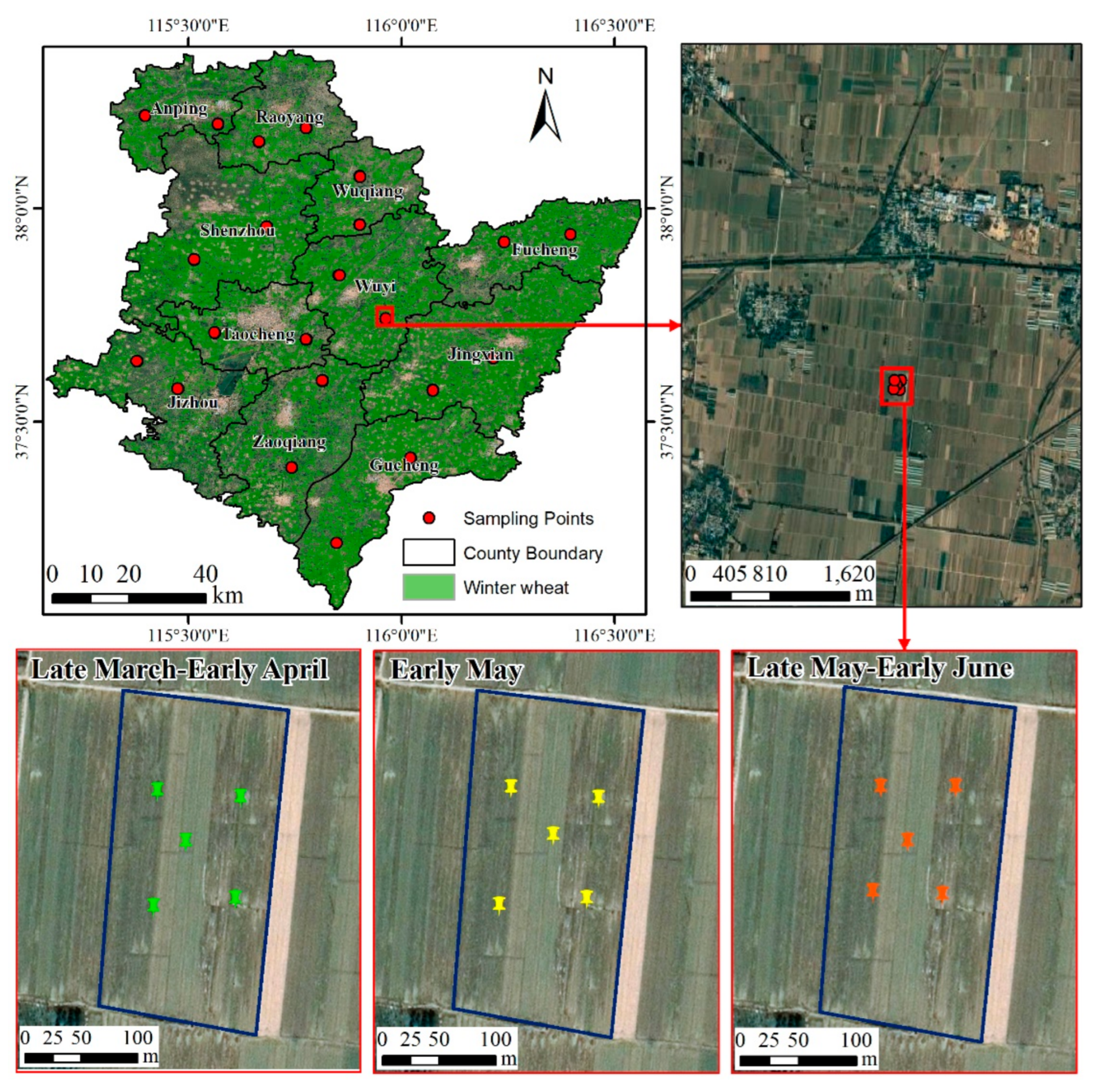
2.2. Field Observation Data

As shown in Figure 1, field campaigns were conducted at Hengshui city from late March to early April, early May, and from late May to early June, corresponding to the jointing, heading, and milk-maturity stage of winter wheat. LAI and above-ground biomass (AGB) were measured the first two times, and grain yield was measured in the last experiment. The data were collected on 22 fields each time, and each field contained five sample sites. Each sampling was carried out within the range of 1 m × 1 m. LAI was measured five times in each sample site with the LI-COR LAI-2200 plant canopy analyzer. AGB and grain yield per unit area were estimated by multiplying the plant density and average individual plant measurements.

2.3. Remote-Sensing Data

Sentinel-2 consists of two polar-orbiting satellites, Sentinel-2A/B, launched successfully in June 2015 and March 2017, respectively. The satellite is equipped with an optoelectronic multispectral sensor for surveying with a temporal resolution of 10 days and spatial resolution of 10 to 60 m in the visible, near-infrared, and short-wave-infrared spectral zones, including 13 spectral channels. Sentinel-2 can capture the differences in vegetation state, including temporal changes. The Landsat-8, launched on 11 February 2013, consists of two science instruments—the operational land imager (OLI) and the thermal infrared sensor (TIRS). The Landsat-8 OLI includes nine bands with a temporal resolution of 16 days and spatial resolution of 30 m, including a 15 m panchromatic band.
We inverted LAI mainly based on NDVI calculated from Sentinel-2 data, corresponding to the transit dates of every ten days from 9 March to 28 May. In addition, for cloud-covered pixels on the date of NDVI calculation, they were replaced by the median NDVI values of cloud-free Landsat-8 and Sentinel-2 within five days before and after (Figure 2).

2.4. Meteorological Data

Meteorological data from a newly available reanalysis dataset (AgERA5) drove the WOFOST crop growth model. This dataset provides daily gridded surface meteorological data from 1979 as input for agriculture and agroecological studies. This dataset is based on the surface level’s hourly ECMWF ERA5 data [29]. It provides variables with 0.1° × 0.1° spatial resolution, including 10 m wind speed (m·s−1), 2 m relative humidity (%), 2 m temperature (K), precipitation flux (mm·day−1), solar radiation flux (J·m−2·day−1), and vapor pressure (hPa). The AgERA5 dataset can be freely available from https://doi.org/10.24381/cds.6c68c9bb (accessed on 22 March 2021).

3. Methods

The primary process for generating the winter wheat yield map includes three parts, as shown in Figure 3. Firstly, construct the likelihood constraints for the crop growth model. This information is based on county-level yield statistics and field observations on winter wheat’s growth and development variables. Secondly, generate posterior ensembles for each 0.1° × 0.1° weather grid based on the differential evolution adaptive metropolis (DREAM) algorithm. Finally, based on the matching of remote-sensing LAI and the posterior LAI ensembles generated in the previous step, the most matched LAI and corresponding estimated yield per 10 m pixel of each weather grid can be obtained.

3.1. WOFOST Model

The WOrld FOod STudies (WOFOST) model is a mechanistic process-based model that describes crop growth considering crop phenology development, leaf development, light interception, CO2 assimilation, root growth, transpiration, respiration, partitioning of assimilates to the various organs, and dry matter formation, as shown in Figure 4. This study implements the WOFOST model in a Python environment based on the PCSE package (https://github.com/ajwdewit/pcse.git, accessed on 22 March 2021).
To explore the posterior uncertainty of the WOFOST model, the initial range of parameters to be optimized needs to be specified. Since the parameters of WOFOST vary in form (single value/array), in this study, we optimize 10 parameters (IDEM, TSUM1, TSUM2, TDWI, SPAN, SLATB, AMAXTB, FLTB, FOTB, FSTB) in the WOFOST model with nine single-valued variables (β_IDEM, α_TSUM1, α_TSUM2, α_TDWI, α_SPAN, α_SLATB, α_AMAXTB, α_v, β_DVS), as listed in Table 1. The initial values for IDEM, TSUM1, and TSUM2 are observation based, and the others are model default values.

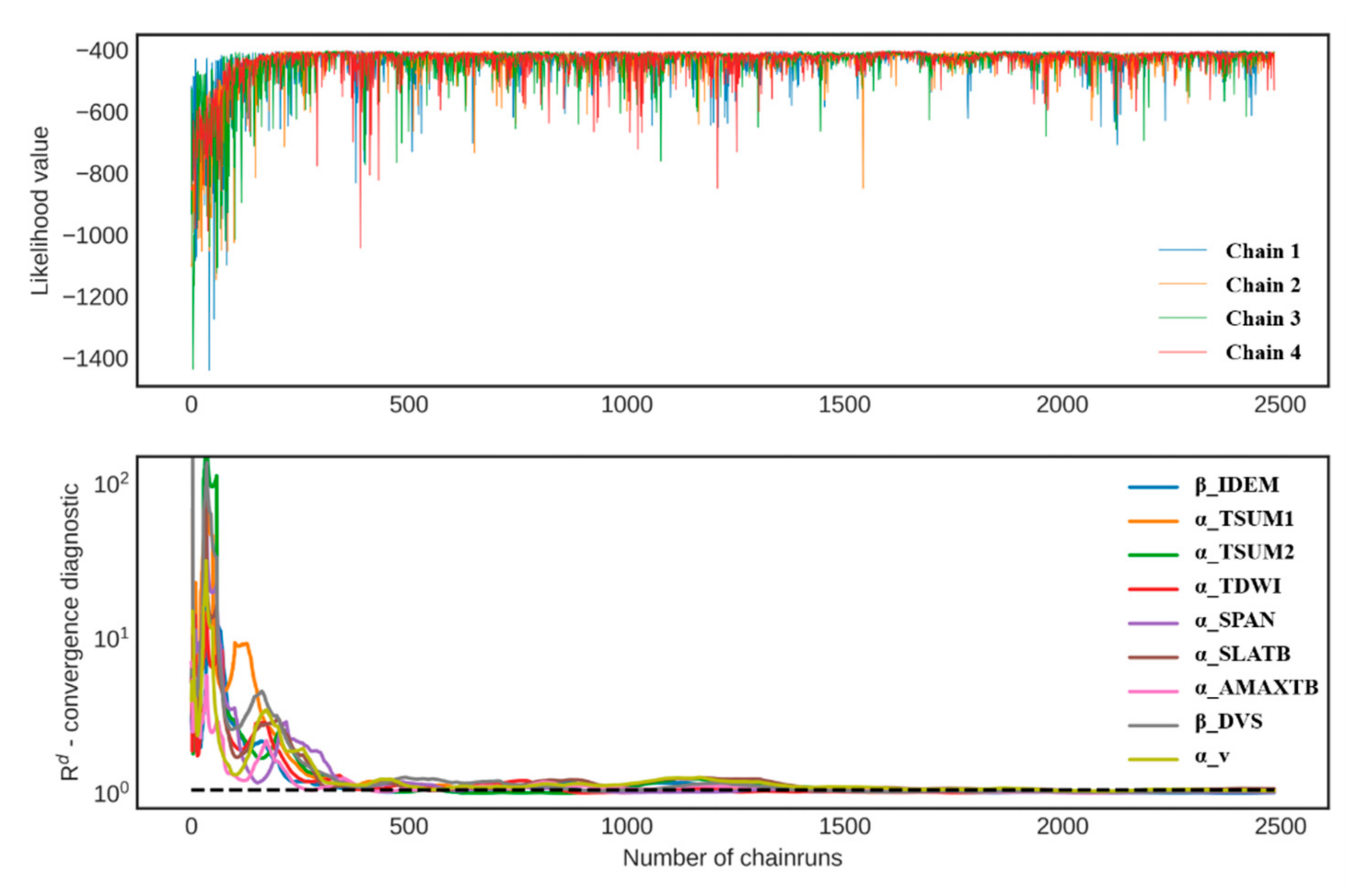
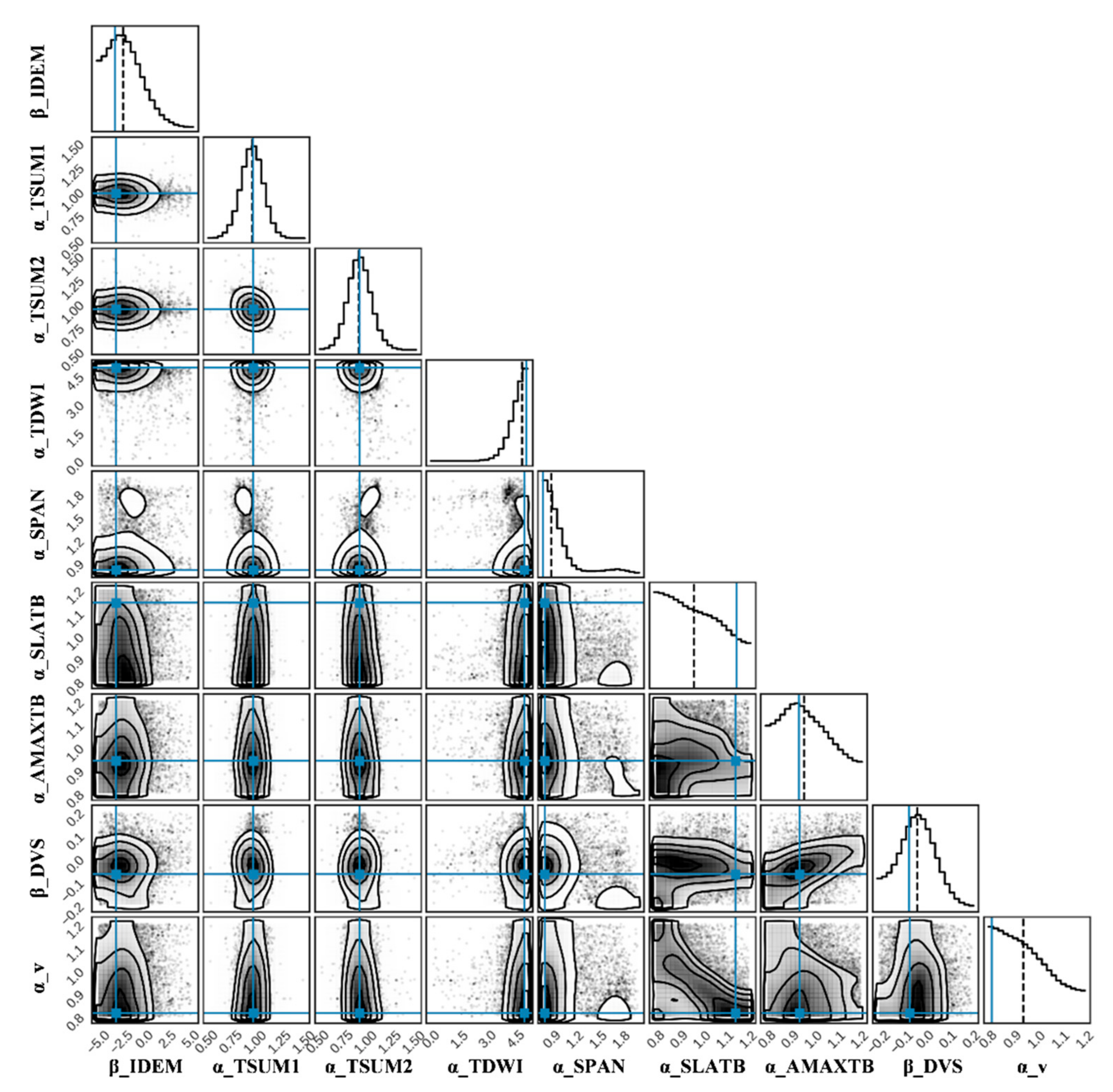
3.2. DREAM Algorithm

The DREAM algorithm is an efficient global Markov chain Monte Carlo (MCMC) method that can explore the posterior uncertainty of complex models even in high-dimensional spaces [31,32].
Overall, the MCMC methods are based on the Bayes theorem and work similarly [4]. Firstly, a Markov chain whose stationary distribution is the posterior of interest is identified, which is actually unknown and can usually hardly be described directly with mathematical formulae. Secondly, sampling from this Markov chain is performed until it converges to an equilibrium distribution, usually diagnosed by some rules of thumb, e.g., the Gelman–Rubin indicator [33]. Finally, these convergent Markov chain samples are essentially sampling from the posterior distribution of interest. We can analyze and infer the posterior distribution quantitatively based on some mathematical statistics of the samples. A significant feature of the DREAM algorithm is that it runs multiple chains in parallel and uses a self-adaptive differential evolution sampling algorithm [34].
Bayesian analysis via MCMC requires specifying parameter priors and the likelihood function. The parameter priors for the nine single-valued variables listed in Table 1 are uniformly distributed (Table 2). The lower and upper bounds are determined after repeated adjustment according to the calibration results. The likelihood function is constructed as follows (Equation (1)):
L = w = 1 N i = DVS ,   LAI , TAGP , TWSO log exp 1 2 ( x i , w μ i ) T Σ i 1 x i , w μ i ( 2 π ) k i Σ i
where x i ,   w is the simulated variables of the WOFOST model; the subscript i and w represent different variables and weather grids. μ i is the county-specific corresponding field or statistical observations of x i ,   w ; Σ i is the covariance matrix of observations. N is the total number of weather grids for a specific county. DVS, LAI, TAGP, and TWSO are development stage, leaf area index, dry above-ground biomass, and dry grain yield. k i is the dimension number(s) of a specific variable. In this study, k DVS is three, corresponding to emergence, flower, and maturity stage, respectively. Additionally, k i for LAI, TAGP, and TWSO are two, two, and one, respectively.
In this study, the DREAM algorithm is implemented in a Python environment based on the SPOTPY package, which enables computational optimization techniques for calibration, uncertainty, and sensitivity analysis techniques of environmental models [35]. This Python package can be publicly available via https://github.com/thouska/spotpy.git (accessed on 22 March 2021).

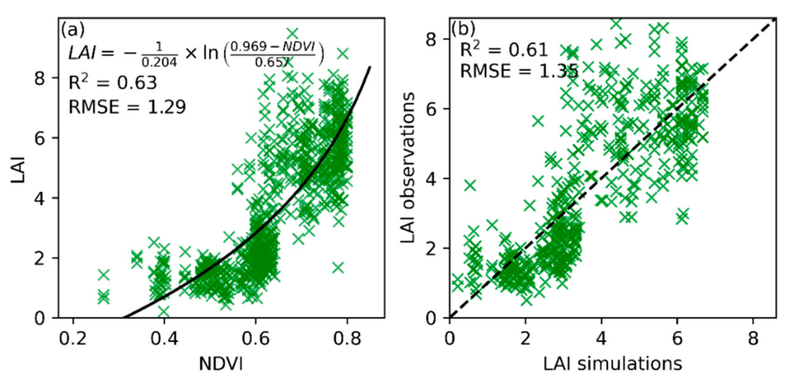
3.3. Remote-Sensing NDVI-Based LAI Inversion

LAI is an important ecological and environmental parameter and is determined by the coverage of leaves per unit of the ground surface. The key to LAI inversion is establishing a relationship with remotely sensed surface reflectance data according to the radiative transfer process of light in the canopy and its spectral response characteristics. Studies have shown a close relationship between remote-sensing NDVI and LAI, and the relationship between them can be described by a modified version of the Beer–Lambert law [36], expressed as Equation (2).
N D V I = N D V I + N D V I 0 N D V I × exp k NDVI × L A I  
where N D V I 0 is the vegetation index of bare soil, N D V I is the value of NDVI when LAI tends to infinity, k NDVI is the extinction coefficient. Therefore, the formula can be approximately expressed as Equation (3).
N D V I = a b × exp c × L A I
where a, b, c are the coefficients to fit the relationship between LAI and NDVI. Additionally, LAI can be expressed as Equation (4).
L A I = 1 / c × ln a N D V I / b
In this study, we use the NDVI calculated from Sentinel-2 and Landsat-8 data and corresponding field-measured LAI to fit their relationship based on Equation (3) and randomly select 60% of the data for modeling and the remaining 40% for validation. The integration of Sentinel-2 and Landsat-8 NDVI calculation and LAI generation based on NDVI are implemented on the Google Earth Engine platform.
In addition, for the pixels with abnormal fluctuations in time-series LAI (by detecting the valley points in the time-series LAI), a smooth cubic spline is performed to reduce the impact of abnormal data (Figure 5). In this case, only outliers are replaced by smooth values, while other values remain unchanged.

3.4. Yield Estimates Based on Bayesian Posterior Ensembles and Remote-Sensing LAI

The meteorological-grid-specified Bayesian posterior ensembles contain one-to-one corresponding LAI and grain yield simulation, which constitute a lookup table with LAI as the input and grain yield as the output (Table 3).
The proposed yield estimation method is an easy-to-understand but effective idea, that is, comparing the time-series LAI retrieved from remote sensing with that in the posterior ensembles one by one, the corresponding yield of the most similar set of LAI is the assimilated yield we are interested in, as illustrated in the lower part of Figure 3. Specifically, for a set of remote-sensing time-series LAI noted as L A I 1 RS ,   L A I 2 RS ,   ,   L A I n 1 RS ,   L A I n RS , the corresponding standard deviation is noted as σ 1 ,   σ 2 ,   ,   σ n 1 ,   σ n . In this study, the standard deviation is set to be 20% of the LAI value. Then, the most similar set of LAI noted as L A I b e s t _ i sim , and the corresponding yield, noted as Y i e l d b e s t _ i , can be estimated as follows:
L A I m × n diff = L A I 1 , 1 sim L A I 1 RS L A I 1 , n sim L A I n RS L A I m , 1 sim L A I 1 RS L A I m , n sim L A I n RS
B = σ 1 0 0 σ n
O b j = diag L A I m × n diff B 1 L A I m × n diff
b e s t _ i = argmin O b j
where L A I m × n diff is the matrix formed by the difference between each set LAI of the Bayesian posterior ensembles and remote-sensing LAI. The subscripts m and n represent the length of Bayesian posterior ensembles and the number of periods for remote-sensing LAI. The diagonal matrix B is the covariance matrix for remote-sensing LAI. The diag ( ) function is used to find the diagonal entries from the given matrix. The argmin ( ) function is used to find the index of the minimum value from the vector O b j .

3.5. Statistical Evaluation

Regression analysis was performed between the simulated and measured value. Three statistical metrics were used to evaluate the goodness of fit, including the coefficient of determination (R2), the root mean square error (RMSE), and the mean absolute percentage error (MAPE), with the metrics calculated as follows:
R 2 = 1 i = 1 n ( y ^ i y i ) i = 1 n y - y i 2 2
RMSE = 1 n i = 1 n y ^ i y i 2
MAPE = 1 n i = 1 n | y ^ i y i y i |     100 %
where y ^ i is the observed data, y i is the simulated data, y ¯ i is the mean value of all simulated data.

4. Results

4.1. Remotely Sensed LAI

The relationship between LAI and NDVI was estimated and validated according to the procedure in Section 3.3, as shown in Figure 6. The LAI of the study area was generated every ten days from 9 March to 28 May, as shown in Figure 7. The maximum LAI value of winter wheat generally appears at the flowering stage. It can be seen that the inversion value of LAI was the largest on 28 April. Across the field observations, the flowering period appeared around 1 May, consistent with the actually observed phenology.

4.2. Bayesian Posterior Uncertainty Exploration of WOFOST with DREAM Method

The Gelman–Rubin diagnostic can be used to check the convergence of MCMC samplers and estimators with the convergence criteria of 1.05. In this study, four parallel Markov chains were run for parameters exploration of each county, and a typical result is plotted in Figure 8. It can be seen that as the number of samplings increases, the likelihood value increases as a whole, while the Gelman–Rubin diagnostic keeps approaching 1 (ideally, when the MCMC sampling converges, the Gelman–Rubin diagnostic is equal to 1).
Typical results of the posterior prediction of the WOFOST model and their corresponding parameters’ uncertainties after MCMC reaches convergence are shown in Figure 9 and Figure 10. The posterior prediction can vary from the specific observations because the posterior of the parameters and their corresponding simulated variables (the posterior prediction) are the result of combining multiple uncertain observations and crop growth model process constraints under a Bayesian framework. For example, in Figure 9, the given LAI, TAGP, and TWSO are not fully compatible with the WOFOST model. That is, there is no set of parameters that can simulate this set of observations simultaneously, which may be due to errors in some of the observations or the inherent deficiencies of the crop growth model. In this case, a compromise result will be achieved. The full posterior as a contour plot and the marginalized posteriors are shown in Figure 10. It can provide various information about different parameters and between parameters. For example, we can see strongly Gaussian shapes of the posteriors in the contour plots for parameters α_TSUM1 and α_TSUM2. We can also notice negative correlation between α_SLATB and α_v, which actually reflects the “equivalence” of SLATB and FLTB in the regulation of LAI in the WOFOST model. Although we focus more on the calibration of models with Bayesian uncertainty, we can evaluate the calibrated variables of our interest by the maximum likelihood simulation results obtained from MCMC sampling, as shown in Figure 11. The model simulation results for each meteorological grid are compared with LAI measurements and county yield statistics corresponding to μ LAI and μ TWSO in Equation (1) with R2 equal to 0.93 and 0.63, and MAPE equal to 11% and 2%, respectively.

4.3. Yield Estimation Accuracy Evaluation and Uncertainty Analysis

The final yield map of winter wheat shows a reasonable spatial distribution. It can reflect the field-level and even within-field variability, and compared with the field measurements, the MAPE for 19 of all 22 fields was less than 15%, as shown in Figure 12. In addition to statistical validation within each field, statistical evaluations were also performed within the county and the entire study area. According to field observations, compared with the other eight counties, three out of eleven counties had more wheat lodging (counties bordered by red lines in Figure 12 and Figure 13); consistently, the validations in these counties have poorer correlation or accuracy, as shown in Figure 13. The estimated yield for all fields, except for the area with lodging of wheat, agrees well with the field measurements with R2, MAPE, and RMSE equal to 0.29, 7.20%, and 574 kg/ha, as shown in Figure 14.

5. Discussion

5.1. Can Yield Variability Be Explained by LAI?

As can be seen from the subgraph in the lower right corner of Figure 12, the pixels at the boundaries of the fields often correspond to low-yield areas, which is the easiest situation to understand—the simulated low-yield is the result of the overall low time-series LAI caused by mixed pixels. In the crop growth model WOFOST, LAI is the basis for photosynthesis, dry matter accumulation, and yield formation. Yield is not only related to the daily LAI value but also to its peak position, time series shape, etc. Therefore, the proposed method is essentially based on the calibrated crop growth model under field measurements and yield statistics.
There is still some uncertainty in the relationship between LAI and yield, as there are various influencing factors, which are not well represented by the model. It can be seen from Figure 13 that the simulated yield tends to overestimate the field-level low yield, especially for those in the lodging area. Since the generated posterior crop simulation ensemble, which is composed of the time-series LAI and the corresponding final yield, is simulated based on the average growth state by the crop growth model, the occurrence of agricultural hazards, e.g., wheat lodging, will disrupt the corresponding relationship between LAI and yield. This can lead to lower LAI matching-based yield estimation accuracy and overestimation for low-yield fields.
Since crop growth models only approximate the actual crop growth situation, the simulation of the response to agricultural hazards, including weeds, diseases, and insects, is not considered for most widely used crop models [5]. Reasonable correlation between crop growth process variables and yield is the key to determining the accuracy for yield estimation based on coupling remote sensing and the crop growth model, but crop stress will greatly increase the uncertainty between them. Therefore, further work is needed to identify agricultural hazards and assess the yield reduction quantitatively based on remote sensing [37,38], improving the generalization ability and accuracy of the proposed framework for regional field-level yield estimation.

5.2. The Role of County-Level Yield Statistics and Their Potential Improvement

In this study, the county-level statistical yield of the previous year and the field growth variable observations of the current year were used to generate a set of possible crop growth states based on the WOFOST model and the MCMC method. We then matched the most likely time-series LAI and the corresponding final yield according to remote-sensing LAI.
The basic logic was building a framework to map the regional yield information into pixel level. However, we selected the previous year’s statistical yield for the following reasons. Firstly, regional statistical yield is relatively stable. It has a strong correlation between the years. For example, in this study, the county-level statistical yield in 2016 can well predict that in 2017 with R2, MAPE, and RMSE equal to 0.69, 2.35%, and 189 kg/ha, as shown in Figure 15. Secondly, the WOFOST model is calibrated with the previous year’s statistical yield and this year’s field observations. The yield simulated from the calibrated model is a compromised value that is closer to the current year’s situation to some extent. Finally, since the county-level statistical yield of the current year will not be released until the second year, the statistical yield of the previous year represents more effective and practical information for yield estimation and forecasting.
In addition, regional-level yield prediction based on different methods tends to have high accuracy [39,40,41], so the method proposed in this study is also capable of field-level yield mapping based on such regional yield forecasting information rather than statistical yield.

5.3. Multiple Remote-Sensing Variables Matching-Based Yield Estimates

The crop model can simulate different state variables, including LAI, biomass, and soil moisture [42,43,44]. In this study, yield matching was only based on LAI retrieved from remote sensing, so the ability to capture yield information is not robust enough; for example, small changes in LAI could result in large yield matching differences. Therefore, a future study can consider more remote-sensing variables for constraints, such as SAR data-based soil moisture, to make full use of the mechanical characteristics of the crop growth model and improve the accuracy of yield estimation.

6. Conclusions

This study presents a rapid data assimilation framework for winter wheat yield estimation at a high spatial resolution with Sentinel-2 data and the WOFOST crop growth model. This core is to fully use the posterior uncertainty under an MCMC method based on yield statistics and field observations. We apply it in a prefecture-level area for field-level yield estimation, and the yield measurements within the field indicate that it can show the overall spatial variability with an error of 7.2%. The proposed framework can provide new perspectives and references for regional crop yield estimation at high spatial resolution in other world areas.

Author Contributions

Conceptualization, J.H. and W.X.; methodology, Y.W.; software, Y.W.; validation, Y.W., H.H. and W.X.; formal analysis, W.X.; investigation, H.H.; resources, W.X.; data curation, Y.W.; writing—original draft preparation, Y.W.; writing—review and editing, H.H.; visualization, H.H.; supervision, J.H.; project administration, J.H.; funding acquisition, J.H. All authors have read and agreed to the published version of the manuscript.

Funding

This research was supported by the National Natural Science Foundation of China (Project No. 41971383), the University College London Research Fund: AMAZING-Advancing Maize Information for Ghana (ST/V001388/1), and Ant Group with the research project “Knowledge and Spatio-temporal Data Driven Crop Growth Model”.

Data Availability Statement

Not applicable.

Acknowledgments

The authors wish to acknowledge Xuecao Li, China Agricultural University, for his valuable advice on language and grammar.

Conflicts of Interest

The authors declare no conflict of interest.

References

  1. Benami, E.; Jin, Z.; Carter, M.R.; Ghosh, A.; Hijmans, R.J.; Hobbs, A.; Kenduiywo, B.; Lobell, D.B. Uniting remote sensing, crop modelling and economics for agricultural risk management. Nat. Rev. Earth Environ. 2021, 2, 140–159. [Google Scholar] [CrossRef]
  2. Moulin, S.; Bondeau, A.; Delecolle, R. Combining agricultural crop models and satellite observations: From field to regional scales. Int. J. Remote Sens. 1998, 19, 1021–1036. [Google Scholar] [CrossRef]
  3. Jin, X.; Kumar, L.; Li, Z.; Feng, H.; Xu, X.; Yang, G.; Wang, J. A review of data assimilation of remote sensing and crop models. Eur. J. Agron. 2018, 92, 141–152. [Google Scholar] [CrossRef]
  4. Huang, J.; Gómez-Dans, J.L.; Huang, H.; Ma, H.; Wu, Q.; Lewis, P.E.; Liang, S.; Chen, Z.; Xue, J.; Wu, Y.; et al. Assimilation of remote sensing into crop growth models: Current status and perspectives. Agr. Forest Meteorol. 2019, 276–277, 107609. [Google Scholar] [CrossRef]
  5. Basso, B.; Cammarano, D.; Carfagna, E. Review of crop yield forecasting methods and early warning systems. In Proceedings of the First Meeting of the Scientific Advisory Committee of the Global Strategy to Improve Agricultural and Rural Statistics, Rome, Italy, 18–19 July 2013; FAO Headquarters: Rome, Italy, 2013. [Google Scholar]
  6. Fritz, S.; See, L.; Bayas, J.C.L.; Waldner, F.; Jacques, D.; Becker-Reshef, I.; Whitcraft, A.; Baruth, B.; Bonifacio, R.; Crutchfield, J.; et al. A comparison of global agricultural monitoring systems and current gaps. Agr. Syst. 2019, 168, 258–272. [Google Scholar] [CrossRef]
  7. Maestrini, B.; Basso, B. Predicting spatial patterns of within-field crop yield variability. Field Crops Res. 2018, 219, 106–112. [Google Scholar] [CrossRef]
  8. Hunt, M.L.; Blackburn, G.A.; Carrasco, L.; Redhead, J.W.; Rowland, C.S. High resolution wheat yield mapping using Sentinel-2. Remote Sens. Environ. 2019, 233, 111410. [Google Scholar] [CrossRef]
  9. Kayad, A.; Sozzi, M.; Gatto, S.; Marinello, F.; Pirotti, F. Monitoring Within-Field Variability of Corn Yield using Sentinel-2 and Machine Learning Techniques. Remote Sens. 2019, 11, 2873. [Google Scholar] [CrossRef] [Green Version]
  10. Skakun, S.; Kalecinski, N.I.; Brown, M.G.L.; Johnson, D.M.; Vermote, E.F.; Roger, J.; Franch, B. Assessing within-Field Corn and Soybean Yield Variability from WorldView-3, Planet, Sentinel-2, and Landsat 8 Satellite Imagery. Remote Sens. 2021, 13, 872. [Google Scholar] [CrossRef]
  11. Segarra, J.; Araus, J.L.; Kefauver, S.C. Farming and Earth Observation: Sentinel-2 data to estimate within-field wheat grain yield. Int. J. Appl. Earth Obs. 2022, 107, 102697. [Google Scholar] [CrossRef]
  12. de Wit, A.; Boogaard, H.; Fumagalli, D.; Janssen, S.; Knapen, R.; van Kraalingen, D.; Supit, I.; van der Wijngaart, R.; van Diepen, K. 25 years of the WOFOST cropping systems model. Agr. Syst. 2019, 168, 154–167. [Google Scholar] [CrossRef]
  13. Jones, J.W.; Hoogenboom, G.; Porter, C.H.; Boote, K.J.; Batchelor, W.D.; Hunt, L.A.; Wilkens, P.W.; Singh, U.; Gijsman, A.J.; Ritchie, J.T. The DSSAT cropping system model. Eur. J. Agron. 2003, 18, 235–265. [Google Scholar] [CrossRef]
  14. Keating, B.A.; Carberry, P.S.; Hammer, G.L.; Probert, M.E.; Robertson, M.J.; Holzworth, D.; Huth, N.I.; Hargreaves, J.N.G.; Meinke, H.; Hochman, Z.; et al. An overview of APSIM, a model designed for farming systems simulation. Eur. J. Agron. 2003, 18, 267–288. [Google Scholar] [CrossRef] [Green Version]
  15. Holzworth, D.P.; Snow, V.; Janssen, S.; Athanasiadis, I.N.; Donatelli, M.; Hoogenboom, G.; White, J.W.; Thorburn, P. Agricultural production systems modelling and software: Current status and future prospects. Environ. Model. Softw. Environ. Data News 2015, 72, 276–286. [Google Scholar] [CrossRef]
  16. Zhuo, W.; Fang, S.; Gao, X.; Wang, L.; Wu, D.; Fu, S.; Wu, Q.; Huang, J. Crop yield prediction using MODIS LAI, TIGGE weather forecasts and WOFOST model: A case study for winter wheat in Hebei, China during 2009–2013. Int. J. Appl. Earth Obs. 2022, 106, 102668. [Google Scholar] [CrossRef]
  17. Huang, J.; Ma, H.; Sedano, F.; Lewis, P.; Liang, S.; Wu, Q.; Su, W.; Zhang, X.; Zhu, D. Evaluation of regional estimates of winter wheat yield by assimilating three remotely sensed reflectance datasets into the coupled WOFOST–PROSAIL model. Eur. J. Agron. 2019, 102, 1–13. [Google Scholar] [CrossRef]
  18. Huang, J.; Sedano, F.; Huang, Y.; Ma, H.; Li, X.; Liang, S.; Tian, L.; Zhang, X.; Fan, J.; Wu, W. Assimilating a synthetic Kalman filter leaf area index series into the WOFOST model to improve regional winter wheat yield estimation. Agr. Forest Meteorol. 2016, 216, 188–202. [Google Scholar] [CrossRef]
  19. Huang, H.; Huang, J.; Li, X.; Zhuo, W.; Wu, Y.; Niu, Q.; Su, W.; Yuan, W. A dataset of winter wheat aboveground biomass in China during 2007–2015 based on data assimilation. Sci. Data 2022, 9, 200. [Google Scholar] [CrossRef]
  20. Kang, Y.; Özdoğan, M. Field-level crop yield mapping with Landsat using a hierarchical data assimilation approach. Remote Sens. Environ. 2019, 228, 144–163. [Google Scholar] [CrossRef]
  21. Ji, F.; Meng, J.; Cheng, Z.; Fang, H.; Wang, Y. Crop Yield Estimation at Field Scales by Assimilating Time Series of Sentinel-2 Data Into a Modified CASA-WOFOST Coupled Model. IEEE Trans. Geosci. Remote Sens. 2021, 60, 4400914. [Google Scholar] [CrossRef]
  22. Silvestro, P.; Pignatti, S.; Pascucci, S.; Yang, H.; Li, Z.; Yang, G.; Huang, W.; Casa, R. Estimating Wheat Yield in China at the Field and District Scale from the Assimilation of Satellite Data into the Aquacrop and Simple Algorithm for Yield (SAFY) Models. Remote Sens. 2017, 9, 509. [Google Scholar] [CrossRef] [Green Version]
  23. Manivasagam, V.S.; Sadeh, Y.; Kaplan, G.; Bonfil, D.J.; Rozenstein, O. Studying the Feasibility of Assimilating Sentinel-2 and PlanetScope Imagery into the SAFY Crop Model to Predict Within-Field Wheat Yield. Remote Sens. 2021, 13, 2395. [Google Scholar] [CrossRef]
  24. Gaso, D.V.; de Wit, A.; Berger, A.G.; Kooistra, L. Predicting within-field soybean yield variability by coupling Sentinel-2 leaf area index with a crop growth model. Agr. Forest Meteorol 2021, 308–309, 108553. [Google Scholar] [CrossRef]
  25. Ziliani, M.G.; Altaf, M.U.; Aragon, B.; Houburg, R.; Franz, T.E.; Lu, Y.; Sheffield, J.; Hoteit, I.; McCabe, M.F. Early season prediction of within-field crop yield variability by assimilating CubeSat data into a crop model. Agr. Forest Meteorol. 2022, 313, 108736. [Google Scholar] [CrossRef]
  26. Dong, J.; Fu, Y.; Wang, J.; Tian, H.; Fu, S.; Niu, Z.; Han, W.; Zheng, Y.; Huang, J.; Yuan, W. Early-season mapping of winter wheat in China based on Landsat and Sentinel images. Earth Syst. Sci. Data 2020, 12, 3081–3095. [Google Scholar] [CrossRef]
  27. Zhao, G.; He, D.; Yao, S. Heibei Rural Statistical Yearbook 2017; China Statistics Press: Beijing, China, 2017. [Google Scholar]
  28. Zhao, G.; He, D.; Yao, S. Heibei Rural Statistical Yearbook 2018; China Statistics Press: Beijing, China, 2018. [Google Scholar]
  29. Hersbach, H.; Bell, B.; Berrisford, P.; Hirahara, S.; Hor, A.; Nyi, A.A.S.; Mu, N.; Oz-Sabater, J.I.N.; Nicolas, J.; Peubey, C.; et al. The ERA5 global reanalysis. Q. J. R. Meteorol. Soc. 2020, 146, 1999–2049. [Google Scholar] [CrossRef]
  30. de Wit, A.; Boogaard, H.L.; Supit, I.; van den Berg, M. System Description of the WOFOST 7.2 Cropping Systems Model.; Wageningen Environmental Research: Wageningen, The Netherlands, 2020. [Google Scholar]
  31. Vrugt, J.A. Markov chain Monte Carlo simulation using the DREAM software package: Theory, concepts, and MATLAB implementation. Environ. Model. Softw. Environ. Data News 2016, 75, 273–316. [Google Scholar] [CrossRef] [Green Version]
  32. Laloy, E.; Vrugt, J.A. High-dimensional posterior exploration of hydrologic models using multiple-try DREAM (ZS) and high-performance computing. Water Resour. Res. 2012, 48, W01526. [Google Scholar] [CrossRef] [Green Version]
  33. Gelman, A.; Carlin, J.B.; Stern, H.S.; Dunson, D.B.; Vehtari, A.; Rubin, D.B. Bayesian Data Analysis; CRC Press: Boca Raton, FL, USA, 2013. [Google Scholar]
  34. Vrugt, J.A.; Ter Braak, C.J.F.; Diks, C.G.H.; Robinson, B.A.; Hyman, J.M.; Higdon, D. Accelerating Markov Chain Monte Carlo Simulation by Differential Evolution with Self-Adaptive Randomized Subspace Sampling. Int. J. Nonlin. Sci. Num. 2009, 10, 273–290. [Google Scholar] [CrossRef]
  35. Houska, T.; Kraft, P.; Chamorro-Chavez, A.; Breuer, L. SPOTting Model Parameters Using a Ready-Made Python Package. PLoS ONE 2015, 10, e145180. [Google Scholar] [CrossRef]
  36. Baret, F.; Guyot, G. Potentials and limits of vegetation indices for LAI and APAR assessment. Remote Sens. Environ. 1991, 35, 161–173. [Google Scholar] [CrossRef]
  37. Chauhan, S.; Darvishzadeh, R.; Boschetti, M.; Pepe, M.; Nelson, A. Remote sensing-based crop lodging assessment: Current status and perspectives. ISPRS J. Photogramm. 2019, 151, 124–140. [Google Scholar] [CrossRef] [Green Version]
  38. Karthikeyan, L.; Chawla, I.; Mishra, A.K. A review of remote sensing applications in agriculture for food security: Crop growth and yield, irrigation, and crop losses. J. Hydrol. 2020, 586, 124905. [Google Scholar] [CrossRef]
  39. Wang, X.; Huang, J.; Feng, Q.; Yin, D. Winter Wheat Yield Prediction at County Level and Uncertainty Analysis in Main Wheat-Producing Regions of China with Deep Learning Approaches. Remote Sens. 2020, 12, 1744. [Google Scholar] [CrossRef]
  40. Lin, T.; Zhong, R.; Wang, Y.; Xu, J.; Jiang, H.; Xu, J.; Ying, Y.; Rodriguez, L.; Ting, K.C.; Li, H. DeepCropNet: A deep spatial-temporal learning framework for county-level corn yield estimation. Environ. Res. Lett. 2020, 15, 34016. [Google Scholar] [CrossRef]
  41. Jiang, H.; Hu, H.; Zhong, R.; Xu, J.; Xu, J.; Huang, J.; Wang, S.; Ying, Y.; Lin, T. A deep learning approach to conflating heterogeneous geospatial data for corn yield estimation: A case study of the US Corn Belt at the county level. Glob. Chang. Biol. 2020, 26, 1754–1766. [Google Scholar] [CrossRef] [PubMed]
  42. Zhuo, W.; Huang, J.; Xiao, X.; Huang, H.; Bajgain, R.; Wu, X.; Gao, X.; Wang, J.; Li, X.; Wagle, P. Assimilating remote sensing-based VPM GPP into the WOFOST model for improving regional winter wheat yield estimation. Eur. J. Agron. 2022, 139, 126556. [Google Scholar] [CrossRef]
  43. Huang, J.; Tian, L.; Liang, S.; Ma, H.; Becker-Reshef, I.; Huang, Y.; Su, W.; Zhang, X.; Zhu, D.; Wu, W. Improving winter wheat yield estimation by assimilation of the leaf area index from Landsat TM and MODIS data into the WOFOST model. Agr. Forest Meteorol. 2015, 204, 106–121. [Google Scholar] [CrossRef] [Green Version]
  44. Zhuo, W.; Huang, J.; Li, L.; Zhang, X.; Ma, H.; Gao, X.; Huang, H.; Xu, B.; Xiao, X. Assimilating Soil Moisture Retrieved from Sentinel-1 and Sentinel-2 Data into WOFOST Model to Improve Winter Wheat Yield Estimation. Remote Sens. 2019, 11, 1618. [Google Scholar] [CrossRef] [Green Version]
Figure 1. Map of study area and distribution of sampling sites during the growth period. The background is acquired from Google base map. The winter wheat mask is obtained from Dong et al. [26]. The green, yellow, and orange pushpins represent the sampling points from late March to early April, early May, and from late May to early June, respectively. The blue boundary represents the selected fields for sampling.
Remotesensing 14 03727 g001
Figure 2. Schematic diagram of Sentinel-2 and Landsat-8 satellite transits over the study area from the beginning of March to the end of May. The green line indicates complete coverage of the study area, and the gray line indicates partial coverage.
Remotesensing 14 03727 g002
Figure 3. Schematic diagram outlining the major process for winter wheat yield estimation.
Remotesensing 14 03727 g003
Figure 4. Schematic overview of the major processes of the WOFOST model [30].
Remotesensing 14 03727 g004
Figure 5. Schematic diagram of abnormal valley smoothing.
Remotesensing 14 03727 g005
Figure 6. Result of LAI modeling and validation. (a) Relationship between NDVI and LAI of winter wheat in the study area. (b) Validation of the LAI model.
Remotesensing 14 03727 g006
Figure 7. Result of LAI inversion every ten days from 9 March to 28 May in the study area.
Remotesensing 14 03727 g007
Figure 8. Plot of likelihood value and Gelman–Rubin diagnostic with Markov chain runs.
Remotesensing 14 03727 g008
Figure 9. Posterior uncertainty of WOFOST model outputs after the convergence of MCMC.
Remotesensing 14 03727 g009
Figure 10. Posterior uncertainty of WOFOST model parameters after the convergence of MCMC. The subplots on the diagonal of the corner plot show the one-dimensional posterior distributions of calibrated parameters, with a solid blue vertical line to indicate the maximum likelihood value and a dashed black line to indicate the median value of the posterior of parameters. The other density plots are two-dimensional projections of the posterior probability distributions for each pair of parameters.
Remotesensing 14 03727 g010
Figure 11. Model validation with the maximum likelihood results.
Remotesensing 14 03727 g011
Figure 12. Map of estimated winter wheat yield of the study area and MAPE for each validation field.
Remotesensing 14 03727 g012
Figure 13. Scatterplots of the simulated yield and measured yield within fields by county.
Remotesensing 14 03727 g013
Figure 14. Scatterplots of the simulated yield and field yield within fields of all counties except for the area with lodging of wheat.
Remotesensing 14 03727 g014
Figure 15. Scatterplots of the official statistical yield for 2016 and 2017.
Remotesensing 14 03727 g015
Table 1. Initial parameter values used for exploring the posterior uncertainty of the WOFOST model.
ParametersDescriptionInitial ValuesOptimized Values and Implementation
IDEMEmergence date19 October 201619 October 2016 + β_IDEM
TSUM1The thermal time from emergence to
anthesis
650650 × α_TSUM1
TSUM2The thermal time from anthesis to maturity950950 × α_TSUM2
TDWIInitial total crop dry weight5050.0 × α_TDWI
SPANThe life span of leaves growing at an
average temperature of 35 °C
31.331.3 × α_SPAN
SLATBSpecific leaf area as a function of
development stage
[0.00, 0.00212,[0.00, 0.00212 × α_SLATB,
0.50, 0.00212,0.50, 0.00212 × α_SLATB,
2.00, 0.00212]2.00, 0.00212 × α_SLATB]
AMAXTBMaximum CO2 assimilation rate as a function of development stage of the crop[0.00, 35.83,[0.00, 35.83 × α_AMAXTB,
1.00, 35.83,1.00, 35.83 × α_AMAXTB,
1.30, 35.83,1.30, 35.83 × α_AMAXTB,
2.00, 4.48]2.00, 4.48 × α_AMAXTB]
FLTBFraction of total dry matter to leaves as a function of DVS[0.000, 0.650,[0.000, 0.650 × α_v,
0.100, 0.650,0.100, 0.650 × α_v,
0.250, 0.700,0.250, 0.700 × α_v,
0.500, 0.500,0.500, 0.500 × α_v,
0.646, 0.300,0.646, 0.300 × α_v,
0.950, 0.000,0.950 + β_DVS, 0.000,
2.000, 0.000]2.000, 0.000]
FOTBFraction of total dry matter to storage
organs as a function of DVS
[0.000, 0.000,[0.000, 0.000,
0.950, 0.000,0.950 + β_DVS, 0.000,
1.000, 1.000,1.000 + β_DVS, 1.000,
2.000, 1.000]2.000, 1.000]
FSTBFraction of total dry matter to stems as a function of DVS[0.000, 0.350,[0.000, 1 − 0.650 × α_v,
0.100, 0.350,0.100, 1 − 0.650 × α_v,
0.250, 0.300,0.250, 1 − 0.700 × α_v,
0.500, 0.500,0.500, 1 − 0.500 × α_v,
0.646, 0.700,0.646, 1 − 0.700 × α_v,
0.950, 1.000,0.950 + β_DVS, 1.000,
1.000, 0.000,1.000 + β_DVS, 0.000,
2.000, 0.000]2.000, 0.000]
Table 2. Lower and upper bound for the optimized variables.
Optimized VariablesFirst GuessLower BoundUpper Bound
β_IDEM0−55
α_TSUM110.51.5
α_TSUM210.51.5
α_TDWI105
α_SPAN10.82.0
α_SLATB10.81.2
α_AMAXTB10.81.2
α_v10.81.2
β_DVS0−0.20.2
Table 3. The lookup table is constituted by the Bayesian posterior ensembles. The subscripts m and n represent the length of Bayesian posterior ensembles and the number of periods for remote-sensing LAI.
LAIYield
L A I 1 sim = L A I 1 , 1 sim , L A I 1 , 2 sim , , L A I 1 , n 1 sim , L A I 1 , n sim Yield1
L A I 2 sim = L A I 2 , 1 sim , L A I 2 , 2 sim , , L A I 2 , n 1 sim , L A I 2 , n sim Yield2
L A I m 1 sim = L A I m 1 , 1 sim , L A I m 1 , 2 sim , , L A I m 1 , n 1 sim , L A I m 1 , n sim Yieldm−1
L A I m sim = L A I m , 1 sim , L A I m , 2 sim , , L A I m , n 1 sim , L A I m , n sim Yieldm
Publisher’s Note: MDPI stays neutral with regard to jurisdictional claims in published maps and institutional affiliations.

