Article

Real-Time Solution of Unsteady Inverse Heat Conduction Problem Based on Parameter-Adaptive PID with Improved Whale Optimization Algorithm

1
Shannxi Key Laboratory of Complex System Control and Intelligent Information Processing, Xi’an University of Technology, Xi’an 710048, China
2
School of Automation and Information Engineering, Xi’an University of Technology, Xi’an 710048, China
*
Author to whom correspondence should be addressed.
Energies 2023, 16(1), 225; https://doi.org/10.3390/en16010225
Submission received: 17 November 2022 / Revised: 15 December 2022 / Accepted: 21 December 2022 / Published: 25 December 2022
(This article belongs to the Section J1: Heat and Mass Transfer)

Abstract

:
To solve the problem of the common unsteady inverse heat conduction problem in the industrial field, a real-time solution method of improving the whale optimization algorithm (IWOA) and parameter-adaptive proportional-integral-differential (PID) is proposed in the paper. A feedback control system with IWOA-PID, which can inversely solve the boundary heat flux, is established. The deviation between the calculated temperature and the measured temperature of the measured point obtained by solving the direct heat conduction problem (DHCP) is used as the system input. The heat flux which is iteration-solved by IWOA-PID is used as system output. The method improves the initial solution distribution, global search capability and population diversity generalization of the traditional whale optimization algorithm (WOA), which effectively improves the parameter-adaptive capability of PID. The experimental results show that the solution method of inverse heat transfer proposed in the paper can accurately retrieve the variation of the boundary heat flux in real time and has good resistance and self-adaptability.

1. Introduction

In special industrial environments, such as crystal growth, equipment manufacturing, aerospace, metallurgical forging, etc., the heat conduction information and the characteristic parameters of key parts of production equipment are difficult to obtain. The common method is to estimate the unknown characteristic parameters based on some known temperature information in the heat conduction system, which is called the inverse heat conduction problem (IHCP). At present, the inverse heat transfer problem is more and more widely used in industry, so it is very important to study an efficient, accurate and robust method to solve the IHCP problem.
Because of the temperature attenuation in the heat conduction process, a small temperature error may lead to instability in the inverse heat conduction calculation. For the unsteady IHCP, scholars have improved the solution strategy of the IHCP from different perspectives, including the Tikhonov regularization method [1], the conjugate gradient (CG) method [2], the particle swarm optimization (PSO) method [3], the hybrid method based on the (PSO), the normal distribution method, the finite element method (FEM) [4], the adaptive neuro-fuzzy inference system (ANFIS) [5], and so on.
All above methods are full-domain inversion algorithms, which are not suitable for online real-time estimation of thermal boundary conditions. In order to improve the real-time performance of thermal boundary estimation, Xiong et al. [6] proposed the sequential function specification method and finite volume method to predict the convective heat transfer coefficients of fluids in two-dimensional pipes in real time. Qi et al. [7,8] proposed an unscented Kalman filter (UKF) and applied it to nonlinear inverse heat conduction problems with an unscented smoother. Many scholars use the method of neural networks to solve the IHCP. For example, Huang et al. [9] uses artificial neural networks combined with Tikhonov regularization to retrieve the heat flux of a three-dimensional unknown surface. Najafi et al. [10] used artificial neural networks as digital filters to achieve real-time estimation of the boundary heat flux. However, this approach requires a large amount of data to train the model, including the nonlinear mapping relationship between heat flow and temperature, to ensure the accuracy of the model.
In recent years, some scholars applied feedback control to study IHCP. Wang et al. [11] proposed a multi-model adaptive inverse (MMAI) method to estimate the heat flux distribution of a nonlinear heat transfer system. It can update the prediction model of a linear heat transfer system in real time and has a strong self-adaptive ability. Sun et al. [12] combined the decentralized fuzzy inference method and the sequential quadratic programming method to estimation of thermal boundary conditions and thermal physical properties parameters in real time. The experiment showed good results. Wan et al. [13] transformed the unsteady IHCP into a kind of PID control problem. The PID controller is driven by the deviation between the output of the DHCP and the measured temperature. Wan et al. [14] proposed an adaptive PID inverse algorithm implemented using a single neuron to estimate the boundary conditions. These studies improve the stability of the solution of the IHCP and open up a new research direction of the problem.
A real-time solution of IHCP using IWOA and parameter-adaptive PID is proposed in the paper for the solution of unsteady one-dimensional IHCP. The method takes the deviation of the measured point temperature as input, the estimated boundary heat flux as output, and the calculated temperature based on heat flux as feedback. The IWOA is used to adapt the PID controller parameters in real time to ensure the minimum difference between the measured temperature and the reconstructed temperature. The experimental results show that the proposed method has good real-time performance, simple structure, strong robustness, and high engineering application value.

2. Mathematical Model

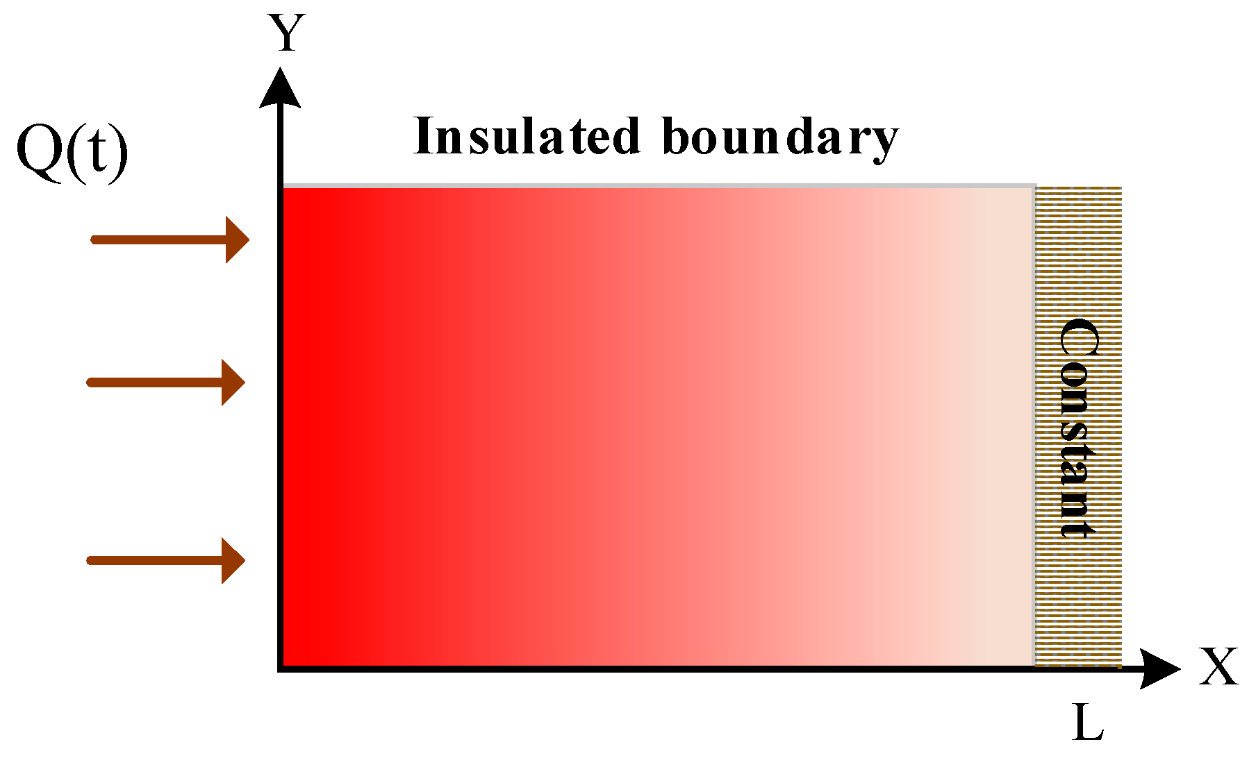
2.1. Thermal System Model

In the paper, the IHCP of heat conduction system is studied. A schematic diagram of heat conduction is shown in Figure 1. The left boundary is the uniformly distributed heat flux boundary varying with time, the right boundary is the constant temperature boundary, and all other boundaries are insulation boundaries. Assuming that the material properties of the system do not change with temperature, there is no obvious temperature difference in the y-axis at any position during heat conduction. Therefore, the heat transfer system can be simplified to one-dimensional heat conduction. The governing equation of one-dimensional heat conduction is as follows:
T ( x , t ) t = α T 2 ( x , t ) x 2 , 0 < x < L , t > 0
The boundary conditions are as follows:
T ( x , 0 ) = T 0 ( x ) , 0 < x < L
λ T ( x , t ) x | x = L = 0
λ T ( x , t ) x | x = 0 = q ( t )
T ( x , t ) represents the temperature at position x at time t , q ( t ) represents the boundary heat flow density, L represents the length of the heat transfer system, α represents the thermal diffusion coefficient, λ represents the thermal conductivity, ρ represents the material density, c p represents the specific heat capacity, and T 0 represents the initial temperature.

2.2. Finite Difference Method

In the paper, the finite difference method is used to solve the direct heat conduction problem (DHCP). In the finite difference method, the derivative of the governing equation is replaced by the difference quotient of the function value on the grid node so that the continuous equation is discretized [15,16].
An explicit two-point forward difference format is used to build a system of algebraic equations with the values on the grid nodes as the unknowns:
T i j + 1 T i j Δ t = α T i + 1 j 2 T i j + T i 1 j Δ x
where T i j represents the temperature of the one-dimensional heat transfer system at position i at j moment. The temperature distribution of the heat transfer system at any time can be derived as follows:
T i j + 1 = s T i + 1 j + ( 1 2 s ) T i j + s T i 1 j
s = Δ t α Δ x
where T i j = T ( x i , t j ) , x i = i Δ x , Δ x is the distance step, Δ x = L / I , I represents the number of grid nodes, t j = j Δ t , Δ t is the time step, and s is the stability coefficient.
The time step and the number of grid nodes should be selected appropriately to be able to ensure that s 0.5 . Ensure the stability of the forward difference scheme [17]. The above mathematical model of heat conduction is discretized by the finite difference method. The temperature distribution of the heat transfer system at any time can be obtained by solving.

3. Parametric Adaptive PID Algorithm to Estimate Heat Flux

3.1. Whale Optimization Algorithm

The WOA is an emerging population intelligence optimization algorithm based on the behavior of whales to surround prey [18]. In the WOA, each whale randomly chooses to surround prey or use a vapor bubble net to drive prey and obtains the optimal solution by continuously updating the position. The algorithm has received wide attention from scholars since it was proposed and has been widely used in a variety of fields [19,20].
The mathematical model of the WOA as follows:
D 1 = | C · X ( t ) X ( t ) |
X ( t + 1 ) = X ( t ) B · D 1
where X represents the value of the optimal solution at the current moment, X represents the position vector. C and B represents the coefficient vector, D 1 represents the distance between the individual and the prey. C and B can be shown as
B = 2 v · r v
C = 2 · r
v = 2 2 t T max
where, v is control parameters. T max is maximum number of iterations. r is defined as a random vector in [0, 1].
Whales move in a spiral pattern. The mathematical model is as follows:
X ( t + 1 ) = D 2 · e m l · cos ( 2 π l ) + X ( t )
D 2 = | X X ( t ) |
where D 2 is the distance from the individual whale to the prey, m is a constant, l is a random number in [−1, 1].
When the prey is near, its contraction encircling and spiral update position behavior are carried out simultaneously. The mathematical model is as follows:
X ( t + 1 ) = { X B · D 1 , p < 0.5 D 2 · e m l · cos ( 2 π l ) + X ( t ) , p 0.5
where p is a random number in [0, 1]
When humpback whales search for prey, | B | 1 . The mathematical model is as follows:
D r a n d = | C · X r a n d X |
X ( t + 1 ) = X r a n d B · D r a n d
where X r a n d is the randomly selected whale position vector. D r a n d represents the distance from a randomly selected individual whale to its prey.
At each moment, the optimal parameter is found by global search through the whale optimization algorithm, and this parameter is used as the controller parameter to inverse the load heat flux at the current moment. The iterative cycle is repeatedly iterated to finally obtain the load heat flux variation in the full time.

3.2. Improving the Whale Optimization Algorithm

The whale optimization algorithm has its own shortcomings. First, the distribution of the initial population has a more obvious impact on the algorithm itself. There is also the slow convergence speed, and tendency to fall into the local optimum. To address these shortcomings, four optimization strategies are proposed in this paper to improve the performance of the whale optimization algorithm.

3.2.1. Optimizing the Initial Solution Space

The uniform distribution of the initial solution space can improve the convergence speed of the algorithm and the chaotic sequence has good randomness, which can make the initial solution space more uniformly distributed. The following equation is shown:
x k + 1 = sin ( d π / x k )
where d is the control parameter, d ( 0 , 1 ) .

3.2.2. Segment Control Parameters and Adaptive Weights

In the whale optimization algorithm, the control parameter v decreases with the number of iterations, which can lead to slow convergence and fall into the problem of local optimum. In the early iteration, increasing the control parameter can improve the global search ability of the algorithm, and in the late iteration, decreasing the control parameter can improve the convergence speed of the algorithm. In this paper, the segmented control parameters are used, as shown in the following equation:
{ v = 1 + cos ( π × t T max ) , t 0.5 T max v = cos ( π × t 0.5 T T max ) , t > 0.5 T max
Equation (10) in the coefficient matrix B calculation is updated to the following equation:
B = 2 v · r v
The adaptive weights are used to optimize the trapping process, and the expression is shown below:
w ( t ) = 2 π × tan ( t T )
The position update formula becomes as follows:
X ( t + 1 ) = X r a n d × w B · D r a n d , p < 0.5 , | A | > 1
X ( t + 1 ) = X ( t ) × w B · D 1 , p < 0.5 , | A | 1
X ( t + 1 ) = D 2 ( t ) e m l cos ( 2 π l ) + X ( t ) × ( 1 w ) , p 0.5 , | A | 1
The adaptive weights and segmentation control parameters can change adaptively as the number of iterations increases, enabling the algorithm to converge quickly and improving the global search capability.

3.2.3. Adaptive Learning Factor

To improve the global optimal seeking ability of the algorithm, an adaptive learning factor is added to control the variability of each individual’s learning ability, at the same time, calculating the adaptation degree among individuals and selecting the individuals with higher adaptation degree. The expressions are shown as follows:
x n e w = { x + r a n d ( 0 , 1 ) × ( x x p ) , f ( x p ) < f ( x ) x + r a n d ( 0 , 1 ) × ( x p x ) , f ( x p ) > f ( x )
where r a n d ( 0 , 1 ) represents the learning factor, which represents the difference in learning ability between individuals.

3.2.4. Cauchy Perturbation Strategy

In order to improve the ability of the algorithm to fall into a local optimum, a perturbation is added to the optimal individual, and in this paper, a Cauchy perturbation is introduced, the expression of which is shown as follows:
x n e w ( t ) = x ( t ) × ( 1 + c a u c h y ( 0 , 1 ) )
where x n e w ( t ) represents the new individual after the Cauchy perturbation and c a u c h y ( 0 , 1 ) is the Cauchy distribution function with the following expression:
f ( x ) = 1 π × ( x 2 + 1 ) , x ( , + )
From the above equation, it is clear that the Cauchy distribution function is capable of generating perturbations that are added to the optimal individuals, giving the improved whale optimization algorithm the ability to avoid the local optima.

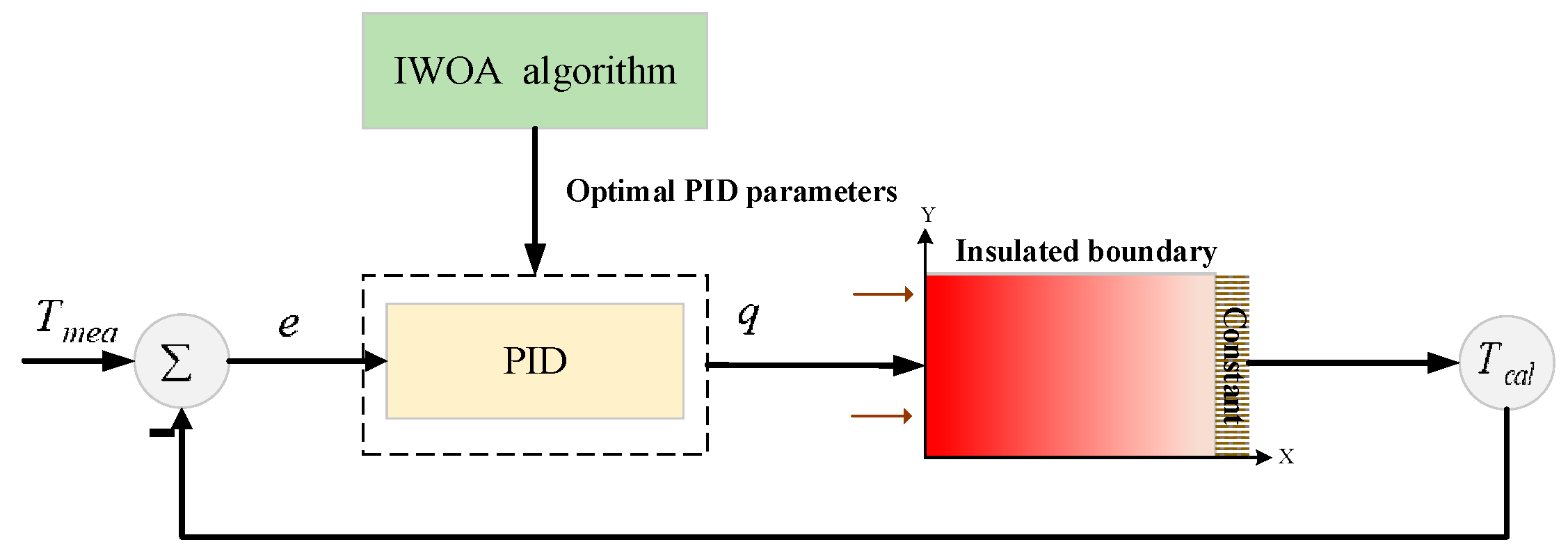
3.3. IWOA-PID Estimated Heat Flux

To the shortcomings of the traditional PID inverse algorithm, such as complex parameter tuning process and poor adaptive ability, a PID method based on the improved whale optimization algorithm (IWOA-PID) is proposed for inverse estimation of the thermal boundary. The schematic diagram of the heat flux inverse estimation by IWOA-PID is shown in Figure 2.
The output of the PID controller is the estimated value of the heat flux at the current moment. We load the estimated value into the DHCP model corresponding to the actual heat transfer system to obtain the estimated temperature at the current moment. The deviation between the estimated temperature and the measured temperature at the current moment is used as the controller input. Then, the accurate heat flux inversion value at the current moment is obtained by iterative calculation. The IWOA is used to adaptively adjust the PID controller parameters at the current moment in each iteration. In the unsteady IHCP, the initial temperature of DHCP at each moment is the temperature distribution under the action of heat flux at the previous moment. Therefore, when inversing the heat flux at the current moment, it is necessary to update the DHCP model by setting the initial temperature to the temperature distribution under the action of heat flow at the previous moment.
In Figure 2, T c a l ( t ) represents the calculated temperature value of the measurement point at the current moment. The direct heat transfer model can be obtained by solving Equations (1) to (4) by using finite difference. The mathematical model is as follows:
q ( t ) = k p e ( t ) + k i 0 t e ( t ) d t + k d d e ( t ) d t
where q represents the estimated value of heat flux at the current moment. k p , k i , and k d represent the proportional coefficient, integral coefficient, and differential coefficient, respectively. e ( t ) represents the input deviation.
The incremental PID algorithm is adopted for the inverse estimation. Compared with the position PID, when the system appears large interference, it will not seriously affect the work of the system [21]. The output of the inverse estimation algorithm at moment k can be replaced by the following equation:
q k = q k 1 + K p ( e ( k ) e ( k 1 ) ) + Δ t K i e ( k ) + K d Δ t ( e ( k ) 2 e ( k 1 ) + e ( k 2 ) )
where K p = k p , K i = Δ t k i , K d = Δ t · k d , the descriptions of k p , k i and k d are given in Formula (28). Equation (29) is referred to as PID below. q k represents the estimated value of heat flux at moment k . Δ t represents the sampling time. e ( k ) represents the deviation between the measured point temperature and the estimated temperature at moment k . The calculation is as follows:
e ( k ) = T m e a ( k ) T c a l ( k )
where T m e a represents the temperature measurement value of the measuring point. T c a l represents the estimated temperature value of the measuring point at the current time.
The input to the PID is e ( k ) , and the output of PID is the estimated boundary heat flux. By estimating the heat flow and solving the DHCP model, the estimated temperature of the measuring point is obtained. Update e ( k ) by Equation (30). The deviation between the measured point temperature and the estimated point temperature decreases. Adaptive adjustment of PID parameters using IWOA. The agent position is updated according to the position vector between the optimal position and its own position until the optimal PID parameter is finally found. The objective function of the IWOA is shown as
M i n ( k = 1 K e ( k ) 2 + α · q ( k ) 2 ) , x R m
where x is the vector of independent variables of the objective function, x = [ K p K i K d ] T . q ( k ) is the historical estimate of heat flux at the current moment. The introduction of q ( k ) into the objective function ensures the stability of the heat flux. α is the regularization parameter. We eliminate the controller input deviation as soon as possible when estimating the heat flux at the current moment.
Based on the above analysis, the steps of the IWOA-PID algorithm for heat flux estimation of the heat transfer system are as follows:
Step1: Set the thermal physical parameters of DHCP model.
Step2: Optimization of PID parameters for the current moment using IWOA at the K moment. Obtain the optimal k p , T i , T d .
Step3: According to the known heat flow change at the previous moment. Obtain the initial temperature at the current moment by solving the heat conduction model and update the DHCP model.
Step4: According to e ( k ) , the heat flux estimate will be obtained, and the measured point temperature estimate will be obtained through the DHCP process.
Step5: Update e ( k ) based on the deviation between the measured point temperature estimate obtained in the previous step and the measured point temperature at the current moment, and return to Step4, decreasing e ( k ) until the heat flux is obtained at K moment.
Step6: Return to Step3 until the iteration is completed, and obtain the heat flow variation in the full time.

4. Experiment and Analysis

4.1. Model Validation

In order to verify the effectiveness and accuracy of the proposed method, the experimental scheme of the literature [22] is simulated in the paper to investigate the one-dimensional unsteady IHCP. The diagram of the experimental device is shown in Figure 3. The test plate has 80 mm width, 96 mm height and 20 mm. One side of the test plate uses a thin mica thermofoil heater, with the other side subjected to a constant temperature by circulating cooling water from a high heat removal capacity water bath. All other sides of the test plate are heavily insulated in order to ensure unidirectional heat transfer. Details can be found in reference [22], and through the data acquisition (DAQ) device to obtain the temperature measurement information. The thermal physical parameters of the experiment are as follows: λ = 40 W / ( m · K ) , ρ c p = 4 10 6 J / ( m 3 · k ) , L = 0.025 m , initial temperature T 0 = 20   ° C , time step Δ t = 0.01 s , space step Δ x = 1.3 × 10 3 m .
The following three forms of thermal loads are applied to the heated surface in the paper, respectively:
Q 1 ( t ) = { 0.4 t             k W / m 2 , 0 < t 75 0.4 t + 60               k W / m 2 , t < 150
Q 2 ( t ) = 30 ( 1 e 0.01 t ) k W / m 2
Q 3 ( t ) = 22.5 + 7.5 sgn { sin [ 2 π ( 1 t / 240 ) ] } k W / m 2
where sgn ( x ) is the symbolic function.
sgn ( x ) = { 1 , x > 0 0 , x < = 0
In practical engineering, any measured temperature will have errors, and the errors depend on the values of the measured temperature. Therefore, white noise is added to the theoretical calculated value of the temperature as the realized measured temperature during the validation:
T m e a j = T e x a j + σ ω
where σ is the standard deviation of the measurement error. ω is a standard normally distributed random number with zero mean and zero standard deviation within the confidence interval [ 2.576 , 2.576 ] . The confidence coefficient is 99%. T e x a j represents the temperature of the measurement point obtained by solving the heat conduction model by finite difference at time j , which is the exact temperature.
To analyze the measurement error, S q and S T are introduced.
S q = 1 k 1 k = 1 K ( q k q e x a k ) 2
S T = 1 k 1 k = 1 K ( T m e a k T c a l k ) 2
The heat flux of the above three different types is applied to the heat transfer system and the temperature at the measurement point is obtained using the finite difference method. The results are shown in Figure 4. The temperature curve in Figure 4 is the calculated value of the measurement temperature at the end position of the heat transfer system. The temperature at the measuring point changes continuously with the change in heat load. There is a significant delay in the temperature change of the measurement point with respect to the change of the heat flux because the temperature of the measurement point is some distance away from the heated end, and the heat diffusion needs some time, the length of which usually depends on the material properties.
Select the location of the measurement point TC1 at 0.02 m . Measurement errors Δ T max is 0.2   ° C . The exact matching method (EMM) [23], WOA-PID and our method were respectively used to estimate the above three kinds of heat flux. The results of the inverse heat flux change at the heated end are shown in Figure 5a,c,e. From Figure 5, it can be seen that the IHCP proposed in the paper can accurately inverse the change of the actual loaded heat flux, and the inverse results of EMM and WOA-PID have a large error with the actual value. Thus, the effectiveness of our method in solving the IHCP is demonstrated. The TC1 temperature reconstruction curves of the measurement points under the three heat fluxes are obtained by our method as shown in Figure 5b,d,f. It can be seen that the temperature of the measured point reconstructed by our method is almost consistent with the actual temperature. The inverse heat flux error S q and temperature reconstruction error S T in three heat flux forms are shown in Table 1. The accuracy of our method in solving the IHCP is verified by comparing with WOA-PID and EMM algorithms. Compared with WOA-PID and EMM algorithms, both S q and S T of our method are minimal, which proves the accuracy of our method in solving IHCP.
To intuitively describe the improvement of inversion accuracy by the algorithm proposed in this paper, the S q accuracy improvement degree and S T accuracy improvement degree are defined as follows:
I S q = S q _ I W O A P I D S q S q _ I W O A P I D × 100 %
I S T = S T _ I W O A P I D S q S T _ I W O A P I D × 100 %
where S q _ I W O A P I D and S T _ I W O A P I D represent the heat flow inversion error and reconstructed temperature error under the proposed algorithm. The calculation methods of the flow inversion error and reconstructed temperature error are shown in Equation (37). As shown in Table 2, the heat flow is a triangular wave. Compared with the WOA-PID heat flow inversion error, the temperature reconstruction error heat flow inversion error increases by 20.78% and 23.08%. Compared with EMM heat flow inversion error increased by 189%, the temperature reconstruction error heat flow inversion error is increased by 572.53%. It shows that the algorithm can improve the accuracy of inversion.

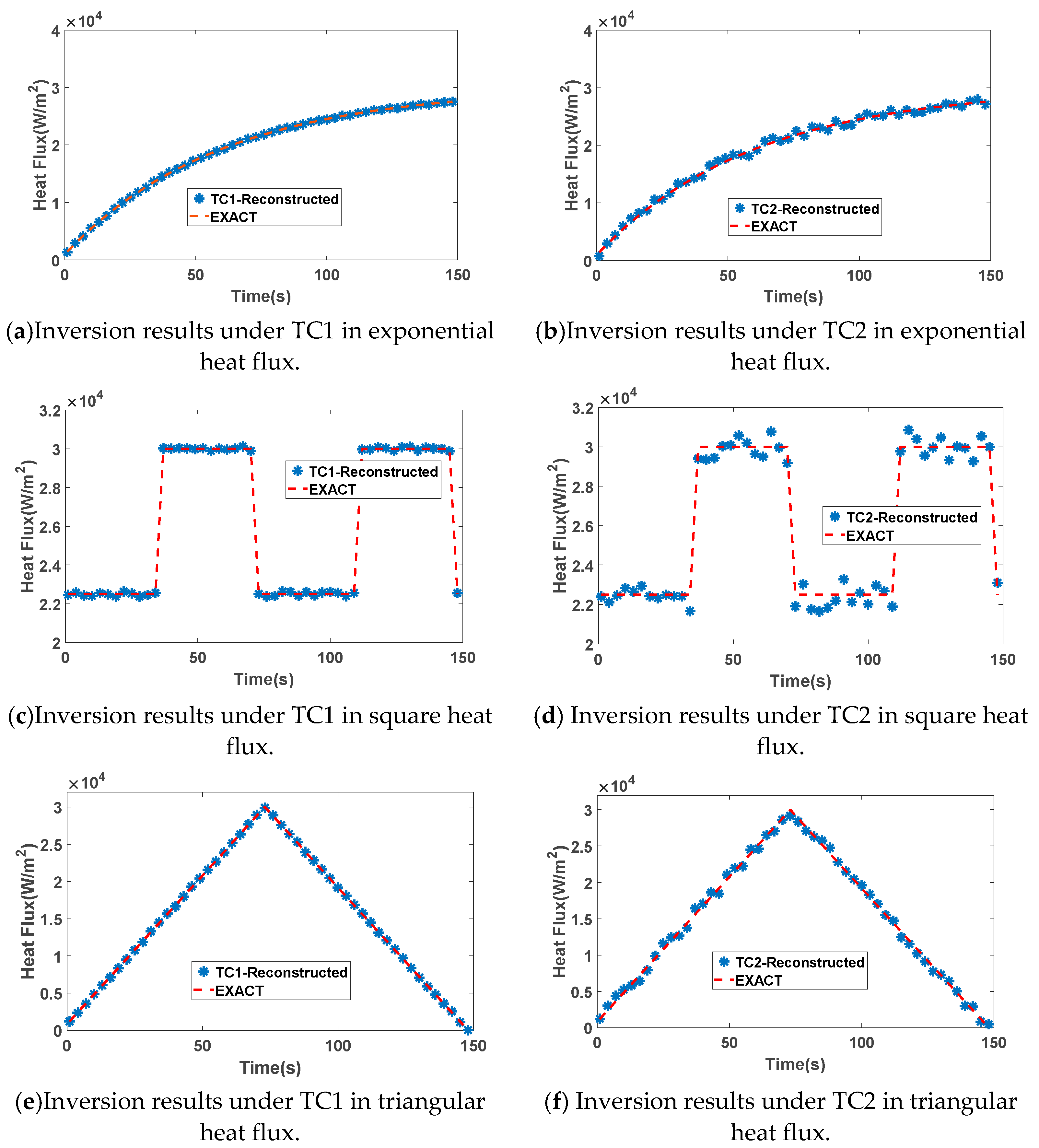
4.2. Influence of Measurement Point Location on Inversion Results

Different positions in the heat transfer system are selected as temperature measurement points. Measurement point one is TC1, and measurement point two is TC2. TC1 is at 0.02 m. TC2 is at 0.025 m. Our method is used for the inversion of the heat fluxes boundary, and the experimental results are shown in Figure 6, in which the measurement error is Δ T max = 0.1   ° C observed.
The inversion results for the three heat flux types at TC1 are shown in Figure 6a,c,e, and the inversion results at TC2 are shown in Figure 6b,d,f.
The changes of the boundary heat flux can be inversed accurately with a small error range before the TC1. When the measurement point location is at the end of the heat transfer system, such as TC2, the inverse errors between the reconstructed values and the exact values are larger than TC1. The inverse error of the two measurement points for the three heat flux types are shown in Table 3. It can be clearly seen that the TC2 is much larger than the errors at TC1. This is due to the significant delay characteristic of thermal diffusion; the longer the distance between the temperature measurement point and the heated end, the more significant the delay in the temperature response.

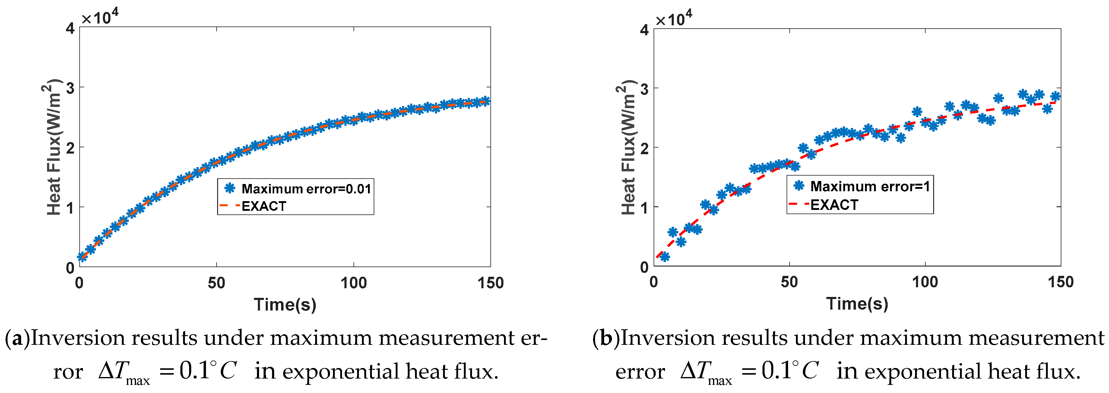
4.3. Influence of Measurement Error on Inversion Results

Taking the exponential heat flux type as an example, the variation of inversion errors at the measurement point position TC at 0.02 m , at the maximum measurement error Δ T max = 0.1   ° C and Δ T max = 1   ° C are shown in Figure 7.
In Figure 7a, the inversion error S q = 93.67 When Δ T max = 0.1   ° C . As shown in Figure 7b, the inversion error S q = 1294 when Δ T max = 1   ° C . The measurement error will also lead to an increase in the heat flow inversion error. The larger the measurement error, the worse the result of the heat flow inversion will be. Therefore, in a practical engineering application, the measurement accuracy of the temperature measurement point should be improved to improve the accuracy of the inversion results.

5. Conclusions

A parameter adaptive PID real-time estimation method of the boundary inverse problem of heat transfer system is proposed based on the idea of the PID feedback control algorithm. For the problem of difficult parameter setting and poor system stability of the traditional PID algorithm, an improved whale optimization algorithm was proposed to adjust the PID parameters adaptively. At each moment, the optimal PID parameters are obtained by improving the whale optimization algorithm and applied to the system to invert the heat flux at the current moment. IWOA-PID can make significant improvements in system stability and rapidity. The experimental results show that the IWOA-PID proposed in the paper can be solved of unsteady inverse heat conduction problems effectively, and the algorithm has good rapidity and can invert the boundary heat flux in real time. Meanwhile, this paper analyzes the influence of the measurement point location and measurement error on the accuracy of the inversion results. The results show that the more distant the location of the measurement point, the inversion error will increase, and the measurement error will affect the accuracy of the inversion results. Additionally, the more distant the location, the more sensitive the accuracy of the inversion results to the measurement error. The effectiveness of the proposed algorithm is verified by experimental analysis. However, the method proposed in this paper is limited to the inverse problem of one-dimensional heat conduction. The inversion conditions are strict. For higher dimensions or multiple boundary conditions, the real-time inversion cannot be realized, as the inversion results will be unstable.

Author Contributions

Methodology, W.H.; Software, J.L.; Data curation, D.L.; Writing—original draft, J.L. All authors have read and agreed to the published version of the manuscript.

Funding

This work are supported by National Natural Science Foundation (NNSF) of China No. 62127809, 62073258, 62003261), Natural Science basic Research Program of Shaanxi Province of China (No. 2020JQ-650), Scientific Research Program Funded of Shaanxi Education Department (No. 20JK0788).

Data Availability Statement

Not applicable.

Conflicts of Interest

The authors declare no conflict of interest.

References

  1. Forooza, S.; Keith, W.; Farshad, K. Optimal combinations of Tikhonov regularization orders for IHCPs. Int. J. Therm. Sci. 2021, 161, 106697. [Google Scholar]
  2. Lu, S.; Heng, Y.; Mhamdi, A. A robust and fast algorithm for three-dimensional transient inverse heat conduction problems. Int. J. Heat Mass Transf. 2012, 55, 7865–7872. [Google Scholar] [CrossRef]
  3. Bangian-Tabrizi, A.; Jaluria, Y. An optimization strategy for the inverse solution of a convection heat transfer problem. Int. J. Heat Mass Transf. 2018, 124, 1147–1155. [Google Scholar] [CrossRef]
  4. Wang, X.; Li, H.; He, L. Evaluation of multi-objective inverse heat conduction problem based on particle swarm optimization algorithm, normal distribution and finite element method. Int. J. Heat Mass Transf. 2018, 127, 1114–1127. [Google Scholar] [CrossRef]
  5. Hsieh, M.C.; Maurya, S.N.; Luo, W.J. Coolant Volume Prediction for Spindle Cooler with Adaptive Neuro-fuzzy Inference System Control Method. Sens. Mater. Int. J. Sens. Technol. 2022, 34, 2447–2466. [Google Scholar] [CrossRef]
  6. Xiong, P.; Qiu, Z.; Lu, Q. Simultaneous estimation of fluid temperature and convective heat transfer coefficient by sequential function specification method. Progress. Nucl. Energy 2020, 131, 103588. [Google Scholar] [CrossRef]
  7. Qi, H.; Wen, S.; Wang, Y. Real-time reconstruction of the time-dependent heat flux and temperature distribution in participating media by using the Kalman filtering technique. Appl. Therm. Eng. 2019, 157, 113667. [Google Scholar] [CrossRef]
  8. Wan, S.; Wang, G.; Chen, H. Application of unscented Rauch-Tung-Striebel smootherto nonlinear inverse heat conduction problems. Int. J. Therm. Sci. 2017, 112, 408–420. [Google Scholar] [CrossRef]
  9. Huang, S.; Tao, B.; Li, J. On-line heat flux estimation of a nonlinear heat conduction system with complex geometry using a sequential inverse method and artificial neural network. Int. J. Heat Mass Transf. 2019, 143, 118491. [Google Scholar] [CrossRef]
  10. Najafi, H.; Woodbury, K.A. Online heat flux estimation using artificial neural network as a digital filter approach. Int. J. Heat Mass Transf. 2015, 91, 808–817. [Google Scholar] [CrossRef]
  11. Wang, G.; Cai, L.; Hong, C. A multiple model adaptive inverse method for nonlinear heat transfer system with temperature-dependent thermophysical properties. Int. J. Heat Mass Transf. 2018, 118, 847–856. [Google Scholar] [CrossRef]
  12. Sun, S. Simultaneous reconstruction of thermal boundary condition and physical properties of participating medium. Int. J. Therm. Sci. 2021, 163, 106853. [Google Scholar] [CrossRef]
  13. Wan, S.; Xu, P.; Wang, K. Real-time estimation of thermal boundary of unsteady heat conduction system using PID algorithm. Int. J. Therm. Sci. 2020, 153, 106395S. [Google Scholar] [CrossRef]
  14. Wan, S.; Wang, K.; Xu, P.; Huang, Y. Numerical and experimental verification of the single neural adaptive PID real-time inverse method for solving inverse heat conduction problems. Int. J. Heat Mass Transf. 2022, 189, 122657. [Google Scholar] [CrossRef]
  15. Arjun, B. The Method of Finite Difference Regression. Open J. Stat. 2018, 8, 49–68. [Google Scholar]
  16. Ming-Chih, L.; Sangbeom, P.; Yunchang, S. An energy stable finite difference method for anisotropic surface diffusion on closed curves. Appl. Math. Lett. 2022, 127, 107848. [Google Scholar]
  17. Ge, Y.; Li, S. Numerical Computation Method for Solving Flow Model of ASP Flooding Based on Full Implicit Finite Difference. Adv. Appl. Math. 2018, 7, 476–493. [Google Scholar] [CrossRef]
  18. Mirjalili, S.; Lewis, A.D. The whale optimization algorithm. Adv. Eng. Softw. 2016, 95, 51–67. [Google Scholar] [CrossRef]
  19. Saeid, S. An effective fake news detection method using WOA-xgbTree algorithm and content-based features. Appl. Soft Comput. 2021, 109, 107559. [Google Scholar]
  20. Anitha, J.; Immanuel, A.; Akila, A. An efficient multilevel color image thresholding based on modified whale optimization algorithm. Expert Syst. Appl. 2021, 178, 115003. [Google Scholar] [CrossRef]
  21. Zhang, Y.; Wei, C.; Chai, T.; Lu, S.; Cui, D. Un-modeled Dynamics Increment Compensation Driven Nonlinear PID Control and Its Application. Acta Autom. Sin. 2020, 46, 1145–1153. [Google Scholar]
  22. Singh, S.K.; Yadav, M.K.; Sonawane, R. Estimation of time-dependent wall heat flux from single thermocouple data. Int. J. Therm. Sci. 2017, 115, 1–15. [Google Scholar] [CrossRef]
  23. Plotkowski, A.; Krane, M.J.M. The Use of Inverse Heat Conduction Models for Estimation of Transient Surface Heat Flux in Electroslag Remelting. J. Heat Transf. 2015, 137, 031301. [Google Scholar] [CrossRef]
Figure 1. Schematic diagram of one-dimensional heat transfer.
Energies 16 00225 g001
Figure 2. Schematic diagram of the heat flux inverse estimation by IWOA-PID.
Energies 16 00225 g002
Figure 3. Schematic diagram of the equipment.
Energies 16 00225 g003
Figure 4. Temperature change of the measurement point under the action of heat flow in three different types. (a) Triangle; (b) square; (c) exponential.
Energies 16 00225 g004
Figure 5. The inversion results and the reconstructed temperature change of measurement points under three different types of heat flux. (a,c,e) are inverse heat fluxes, (b,d,f) are TC1 temperature reconstruction.
Energies 16 00225 g005
Figure 6. Influence of the location of the measurement points on the inversion results under three different types of heat flux. (a,c,e) are inversion heat fluxes under temperature measurement point TC1, (b,d,f) are inversion heat fluxes under temperature measurement point TC2.
Energies 16 00225 g006
Figure 7. Influence of measurement error on inversion results. (a) is inversion result under maximum measurement error Δ T max = 0.1   ° C in exponential heat flux. (b) is inversion result under maximum measurement error Δ T max = 1   ° C in exponential heat flux.
Energies 16 00225 g007
Table 1. Inversion error and reconstruction error under three heat flux types.
Heat FluxIWOA-PIDWOA-PIDEMM
S q S T S q S T S q S T
Triangle type458.27620.7573553.53100.93211.3706 × 1035.0911
Exponential type450.90740.6309492.01420.70541.3348 × 1034.5969
Square type471.33750.7319530.92130.8770686.91122.044
Table 2. Accuracy improvement degree under three heat flux types.
Heat FluxIWOA-PID and WOA-PIDIWOA-PID and EMM
I S q I S T I S q I S T
Triangle type20.78%23.08%189%572.53%
Exponential type9.33%10.56%196%628.62%
Square type12.52%16.54%45.84%179.27%
Table 3. Inversion error under three different types of heat flow.
Heat FluxTC1TC2
Triangle type72.641500.2478
Exponential type73.4419571.5412
Square type78.8352438.1187
Disclaimer/Publisher’s Note: The statements, opinions and data contained in all publications are solely those of the individual author(s) and contributor(s) and not of MDPI and/or the editor(s). MDPI and/or the editor(s) disclaim responsibility for any injury to people or property resulting from any ideas, methods, instructions or products referred to in the content.

