
Mathematical Modelling for Predicting Thermal Properties of Selected Limestone

 and
and
Abstract

1. Introduction
2. Materials and Methods
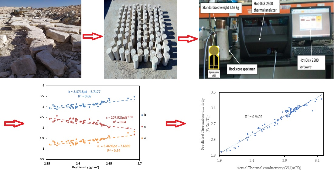
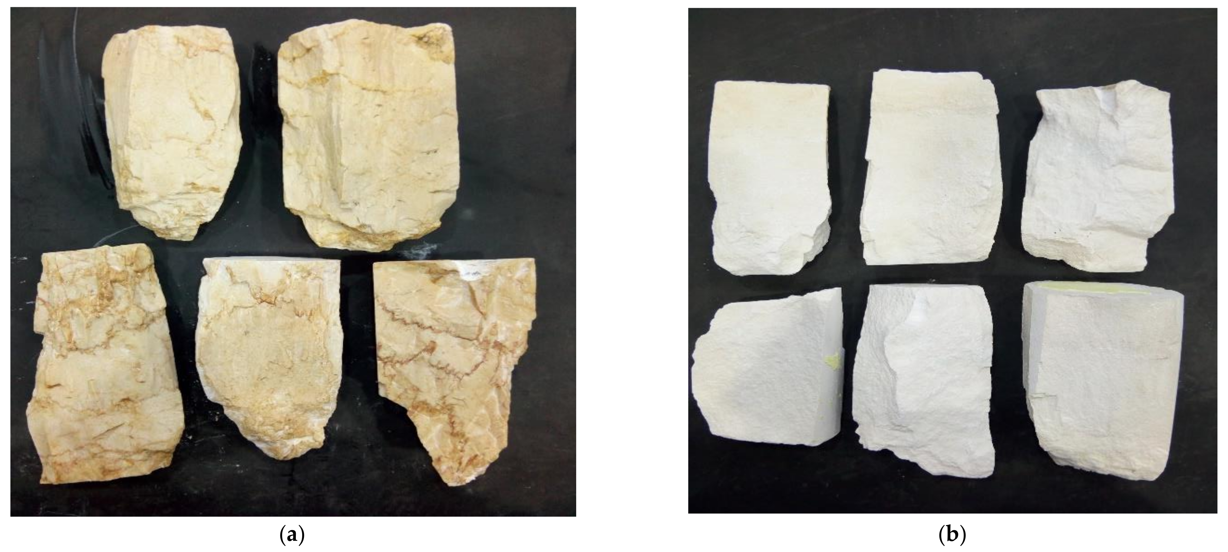
2.1. Rock Specimens Preparation
2.2. Method and Laboratory Tests
2.2.1. Thermal Properties Determination
2.2.2. Physical and Engineering Properties Determination
3. Results and Discussion
3.1. Thermal Properties of Limestone Rock
3.2. Regression Analysis for Predicting Thermal Properties
3.3. Simple Regression Analysis
3.4. Multivariate Regression Analysis
3.5. Artificial Neural Network Analysis
4. Conclusions
- There is a difference in the thermal properties of the included limestone, especially in the specific heat. This is due to the difference in physical and engineering properties, the variance in the abundance of minerals in it, and the variance in porosity.
- The results of an independent samples t-test analysis indicate a statistically significant difference in the thermal, physical, and engineering properties between rocks, where the calculated p-value for each property is close to zero (i.e., less than 0.05).
- The thermal conductivity increases with the increasing thermal diffusivity and decreases with the increasing heat capacity. Increasing conductivity means that further heat will be extracted from the source, which means the diffusivity of absorbed heat become faster. On the other hand, a small conductivity value means that the material mostly absorbs heat, and a small amount of the heat will be transmitted through the medium.
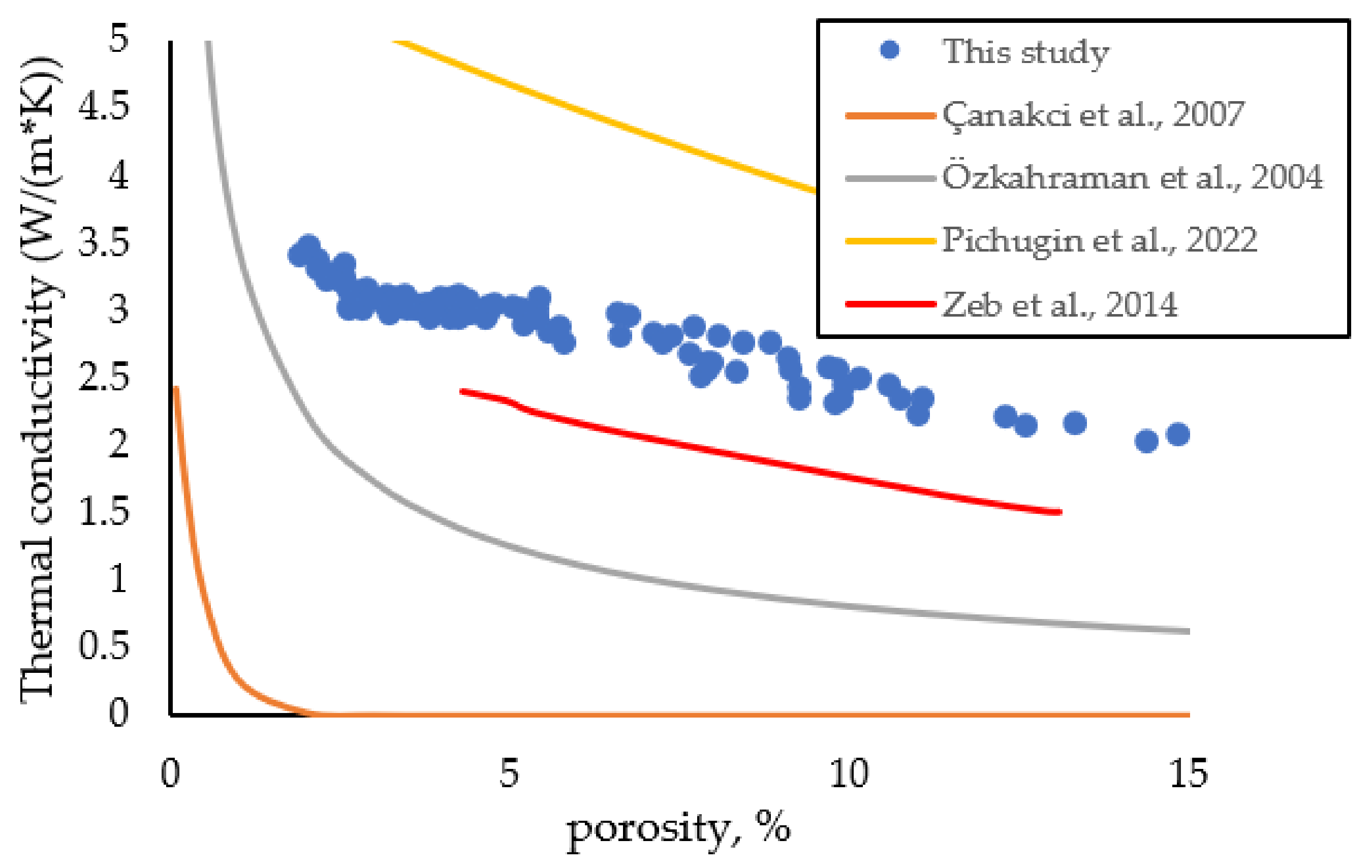
- The low thermal conductivity values for studied rocks compared to some other building stones mean that it can be considered as the best and perfect thermal conductor.
- There is a direct relationship between the conductivity and diffusivity (i.e., an inverse relationship to the specific heat) and the density, hardness, pulse velocity, and rock strength. When the thermal properties are linked with the porosity of the rock, an inverse relationship between the conductivity and diffusivity (i.e., a direct relationship to the specific heat) was observed with the previous properties.
- Indirectly, the thermal properties of the lime building stone can be predicted through a set of mathematical models that relate the thermal properties with the physical and engineering properties. These mathematical models were developed by using regression analysis.
- According to multivariate regression analysis, a strong correlation between thermal properties and rock’s compressive strength was observed, where the UCS was termed in all multivariate regression models; therefore, it can be considered the most important factor affecting the thermal properties of the rock.
- ANN models provide more accurate and better results in terms of R2, RMSE, and applicability on a holdout sample (validation data set), especially for specific heat prediction as opposed to multivariate regression.
Author Contributions
Funding
Institutional Review Board Statement
Informed Consent Statement
Data Availability Statement
Conflicts of Interest
References
- Yaşar, E.; Erdoğan, Y. Strength and Thermal Conductivity in Lightweight Building Materials. Bull. Eng. Geol. Environ. 2008, 67, 513–519. [Google Scholar] [CrossRef]
- Gul, I.H.; Maqsood, A. Thermophysical Properties of Diorites along with the Prediction of Thermal Conductivity from Porosity and Density Data. Int. J. Thermophys. 2006, 27, 614–626. [Google Scholar] [CrossRef]
- Çengel, Y.A. Heat Transfer: A Practical Approach, 2nd ed.; McGraw-Hill: Boston, MA, USA, 2003. [Google Scholar]
- Shi, X. Controlling Thermal Properties of Asphalt Concrete and Its Multifunctional Applications. Master’s Thesis, Texas A&M University, College Station, TX, USA, 2014. [Google Scholar]
- Labus, M.; Labus, K. Thermal Conductivity and Diffusivity of Fine-Grained Sedimentary Rocks. J. Therm. Anal. Calorim. 2018, 132, 1669–1676. [Google Scholar] [CrossRef]
- Robertson, E.C. Thermal Properties of Rocks; US Department of the Interior: Washington, DC, USA; Geological Survey: Reston, VA, USA, 1988.
- Sun, Q.; Lü, C.; Cao, L.; Li, W.; Geng, J.; Zhang, W. Thermal Properties of Sandstone after Treatment at High Temperature. Int. J. Rock Mech. Min. Sci. 2016, 85, 60–66. [Google Scholar] [CrossRef]
- Stylianou, I.I.; Tassou, S.; Christodoulides, P.; Panayides, I.; Florides, G. Measurement and Analysis of Thermal Properties of Rocks for the Compilation of Geothermal Maps of Cyprus. Renew. Energy 2016, 88, 418–429. [Google Scholar] [CrossRef]
- Çanakci, H.; Demirboğa, R.; Karakoç, M.B.; Şirin, O. Thermal Conductivity of Limestone from Gaziantep (Turkey). Build. Environ. 2007, 42, 1777–1782. [Google Scholar] [CrossRef]
- Khandelwal, M. Prediction of Thermal Conductivity of Rocks by Soft Computing. Int. J. Earth Sci. 2010, 100, 1383–1389. [Google Scholar] [CrossRef]
- Jones, M.Q.W. Thermal Properties of Stratified Rocks from Witwatersrand Gold Mining Areas. J. South. African Inst. Min. Metall. 2003, 103, 173–185. [Google Scholar]
- Harmathy, T.Z. Thermal Properties of Concrete at Elevated Temperatures. J. Mater. 1970, 5, 47–74. [Google Scholar]
- Ahadi, M.; Andisheh-Tadbir, M.; Tam, M.; Bahrami, M. An Improved Transient Plane Source Method for Measuring Thermal Conductivity of Thin Films: Deconvoluting Thermal Contact Resistance. Int. J. Heat Mass Transf. 2016, 96, 371–380. [Google Scholar] [CrossRef]
- Troschke, B.; Burkhardt, H. Thermal Conductivity Models Fro Two-Phase Systems. Phys. Chem. Earth 1998, 23, 351–355. [Google Scholar] [CrossRef]
- Clauser, C.; Huenges, E. Thermal Conductivity of Rocks and Minerals. In Rock Physics and Phase Relations: A Handbook of Physical Constants; John Wiley & Sons: Hoboken, NJ, USA, 2013; Volume 3, pp. 105–126. [Google Scholar]
- Boulanouar, A.; Rahmouni, A.; Boukalouch, M.; Samaouali, A.; Géraud, Y.; Harnafi, M.; Sebbani, J. Determination of Thermal Conductivity and Porosity of Building Stone from Ultrasonic Velocity Measurements. Geomaterials 2013, 3, 138–144. [Google Scholar] [CrossRef]
- Özkahraman, H.T.; Selver, R.; Işk, E.C. Determination of the Thermal Conductivity of Rock from P-Wave Velocity. Int. J. Rock Mech. Min. Sci. 2004, 41, 703–708. [Google Scholar] [CrossRef]
- Han, H.; Yin, S. In-Situ Stress Inversion in Liard Basin, Canada, from Caliper Logs. Petroleum 2018, 6, 392–403. [Google Scholar] [CrossRef]
- Maji, V.B.; Sitharam, T.G. Prediction of Elastic Modulus of Jointed Rock Mass Using Artificial Neural Networks. Geotech. Geol. Eng. 2008, 26, 443–452. [Google Scholar] [CrossRef]
- Bui, D.K.; Nguyen, T.N.; Ngo, T.D.; Nguyen-Xuan, H. An Artificial Neural Network (ANN) Expert System Enhanced with the Electromagnetism-Based Firefly Algorithm (EFA) for Predicting the Energy Consumption in Buildings. Energy 2020, 190, 116370. [Google Scholar] [CrossRef]
- Singh, T.N.; Sinha, S.; Singh, V.K. Prediction of Thermal Conductivity of Rock through Physico-Mechanical Properties. Build. Environ. 2007, 42, 146–155. [Google Scholar] [CrossRef]
- Dweirj, M.; Fraige, F.; Alnawafleh, H.; Titi, A.; Dweirj, M.; Fraige, F.; Alnawafleh, H.; Titi, A. Geotechnical Characterization of Jordanian Limestone. Geomaterials 2017, 7, 1–12. [Google Scholar] [CrossRef]
- NRAUT. Geological and Engineering Study of Limestone Suitable for Construction Purposes in the Eastern Part of the Hashemite Kingdom of Jordan; Natural Resources Authority Report; NRAUT: Amman, Jordan, 2003.
- ASTM D4543; Practices for Preparing Rock Core as Cylindrical Test Specimens and Verifying Conformance to Dimensional and Shape Tolerances. ASTM International: West Conshohocken, PA, USA, 2019. [CrossRef]
- He, Y. Rapid Thermal Conductivity Measurement with a Hot Disk Sensor: Part 1. Theoretical Considerations. Thermochim. Acta 2005, 436, 122–129. [Google Scholar] [CrossRef]
- Chen, T.-G.; Yu, P.; Chou, R.-H.; Pan, C.-L. Phonon Thermal Conductivity Suppression of Bulk Silicon Nanowire Composites for Efficient Thermoelectric Conversion. Opt. Express 2010, 18, A467. [Google Scholar] [CrossRef]
- Mirzanamadi, R.; Johansson, P.; Grammatikos, S.A. Thermal Properties of Asphalt Concrete: A Numerical and Experimental Study. Constr. Build. Mater. 2018, 158, 774–785. [Google Scholar] [CrossRef]
- International Society for Rock Mechanics (ISRM). The ISRM Suggested Methods for Rock Characterization, Testing and Monitoring: 2007–2014; Ulusay, R., Ed.; Springer International Publishing: Cham, Switzerland, 2007; ISBN 978-3-319-07712-3. [Google Scholar]
- ASTM D2845; Standard Test Method for Laboratory Determination of Pulse Velocities and Ultrasonic Elastic Constants of Rock. ASTM International: West Conshohocken, PA, USA, 2008.
- ASTM D5873; Standard Test Method for Determination of Rock Hardness by Rebound Hammer Method. ASTM International: West Conshohocken, PA, USA, 2014.
- ASTM D7012; Standard Test Method for Compressive Strength and Elastic Moduli of Intact Rock Core Specimens under Varying States of Stress and Temperatures. ASTM International: West Conshohocken, PA, USA, 2014.
- ASTM D5731; Standard Test Method for Determination of the Point Load Strength Index of Rock and Application to Rock Strength Classifications. ASTM International: West Conshohocken, PA, USA, 2016. [CrossRef]
- Islam, M.R.; Tarefder, R.A. Determining Thermal Properties of Asphalt Concrete Using Field Data and Laboratory Testing. Constr. Build. Mater. 2014, 67, 297–306. [Google Scholar] [CrossRef]
- Cermak, V.; Rybach, L. Thermal Conductivity and Specific Heat of Minerals and Rocks. In Geophysics—Physical Properties of Rocks; Beblo, M., Ed.; Springer: Berlin/Heidelberg, Germany, 1982; pp. 305–343. ISBN 3540110704. [Google Scholar]
- Pechnig, R.; Mottaghy, D.; Koch, A.; Jorand, R.; Clauser, C. Prediction of Thermal Properties for Mesozoic Rocks of Southern Germany. In Proceedings of the European Geothermal Congress, Unterhaching, Germany, 30 May–1 June 2007. [Google Scholar]
- Rajabi, A.; Hosseini, A.; Heidari, A. The New Empirical Formula to Estimate the Uniaxial Compressive Strength of Limestone; North of Saveh a Case Study. J. Eng. Geol. 2017, 11, 159–180. [Google Scholar]
- Mahdiyar, A.; Armaghani, D.J.; Marto, A.; Nilashi, M.; Ismail, S. Rock Tensile Strength Prediction Using Empirical and Soft Computing Approaches. Bull. Eng. Geol. Environ. 2019, 78, 4519–4531. [Google Scholar] [CrossRef]
- Barham, W.S.; Rabab’ah, S.R.; Aldeeky, H.H.; Al Hattamleh, O.H. Mechanical and Physical Based Artificial Neural Network Models for the Prediction of the Unconfined Compressive Strength of Rock. Geotech. Geol. Eng. 2020, 38, 4779–4792. [Google Scholar] [CrossRef]
- Pichugin, Z.; Chekhonin, E.; Popov, Y.; Kalinina, M.; Bayuk, I.; Popov, E.; Spasennykh, M.; Savelev, E.; Romushkevich, R.; Rudakovskaya, S. Weighted Geometric Mean Model for Determining Thermal Conductivity of Reservoir Rocks: Current Problems with Applicability and the Model Modification. Geothermics 2022, 104, 102456. [Google Scholar] [CrossRef]
- Zeb, A.; Misbah; Maqsood, A. Prediction of Effective Thermal Conductivity of Consolidated Porous Materials under Ambient Conditions. Indian J. Phys. 2014, 88, 603–607. [Google Scholar] [CrossRef]
- Chekhonin, E.; Popov, Y.; Romushkevich, R.; Popov, E.; Zagranovskaya, D.; Zhukov, V. Integration of Thermal Core Profiling and Scratch Testing for the Study of Unconventional Reservoirs. Geosciences 2021, 11, 260. [Google Scholar] [CrossRef]
- Feng, X.; Jimenez, R. Bayesian Prediction of Elastic Modulus of Intact Rocks Using Their Uniaxial Compressive Strength. Eng. Geol. 2014, 173, 32–40. [Google Scholar] [CrossRef]
- Pallant, J. SPSS Survival Manual: A Step by Step Guide to Data Analysis Using IBM SPSS; Routledge: London, UK, 2020; ISBN 1003117457. [Google Scholar]
- Larson-Hall, J. A Guide to Doing Statistics in Second Language Research Using SPSS and R; Routledge: London, UK, 2015; ISBN 1315775662. [Google Scholar]
- Hornik, K.; Stinchcombe, M.; White, H. Multilayer Feedforward Networks Are Universal Approximators. Neural Netw. 1989, 2, 359–366. [Google Scholar] [CrossRef]
- Gardner, M.W.; Dorling, S.R. Artificial Neural Networks (the Multilayer Perceptron)—A Review of Applications in the Atmospheric Sciences. Atmos. Environ. 1998, 32, 2627–2636. [Google Scholar] [CrossRef]


| Property | Min. | Max. | Avg. | Standard Deviation | Coefficient of Variation |
|---|---|---|---|---|---|
| k (W/(m × k)) | 1.931 | 3.468 | 2.861 | 0.327 | 11.45 |
| α (mm2/s) | 1.032 | 1.810 | 1.323 | 0.123 | 9.31 |
| c ((MJ)/(m3 × K)) | 1.570 | 2.563 | 2.157 | 0.192 | 8.91 |
| Property | Unit | No. of Specimens | Min. | Max. | Avg. | Standard Deviation | Coefficient of Variation |
|---|---|---|---|---|---|---|---|
| ρd | g/cm3 | 100 | 2.521 | 2.692 | 2.521 | 0.113 | 4.492 |
| Gs | - | 100 | 2.677 | 2.714 | 2.677 | 0.031 | 1.16 |
| Hr | - | 100 | 34.423 | 43.65 | 34.422 | 4.912 | 14.269 |
| UCS | MPa | 100 | 81.341 | 138.39 | 81.341 | 20.448 | 25.139 |
| Is(50) | MPa | 100 | 3.357 | 4.825 | 3.357 | 0.579 | 17.241 |
| n% | - | 100 | 5.845 | 15.924 | 5.846 | 3.265 | 55.87 |
| Vp | m/s | 100 | 5476.3 | 6366.3 | 5476.32 | 618.228 | 11.289 |
| Source 1 | Source 2 | |||||
|---|---|---|---|---|---|---|
| DV | Statistic | Df * | Sig. | Statistic | Df * | Sig. |
| k | 0.082 | 50 | 0.200 | 0.097 | 50 | 0.200 |
| α | 0.118 | 50 | 0.082 | 0.111 | 50 | 0.172 |
| c | 0.102 | 50 | 0.200 | 0.093 | 50 | 0.200 |
| Independent Variable | Unit | Equation (Source 1) | R2 | VAF% | RMSE | Equation (Source 2) | R2 | VAF% | RMSE |
|---|---|---|---|---|---|---|---|---|---|
| ρ d | g/cm3 | k = 3.3716 ρd − 5.7177 c = 207.92 ρd−4.719 α = 3.4696 ρd − 7.6889 | 0.66 0.64 0.64 | 66 62 64 | 0.07 0.09 0.07 | k = 3.1391 ρd − 4.9995 c = −1.9003 ρd + 6.6864 α = 0.9539 ρd − 1.0435 | 0.89 0.90 0.92 | 89 90 92 | 0.11 0.05 0.02 |
| Gs | - | k = 9.0146 (Gs) − 21.314 c= −10.26(Gs) + 30.02 α = 8.8217(Gs) − 22.507 | 0.1 0.1 0.09 | 3.56 14.66 5 | 1.3 1.8 1.7 | k = 14.286 (Gs) − 35.191 c = −9.9973(Gs) + 28.536 α = 4.819 (Gs) − 11.483 | 0.38 0.51 0.48 | 4.51 14.53 3.67 | 19.94 0.87 0.81 |
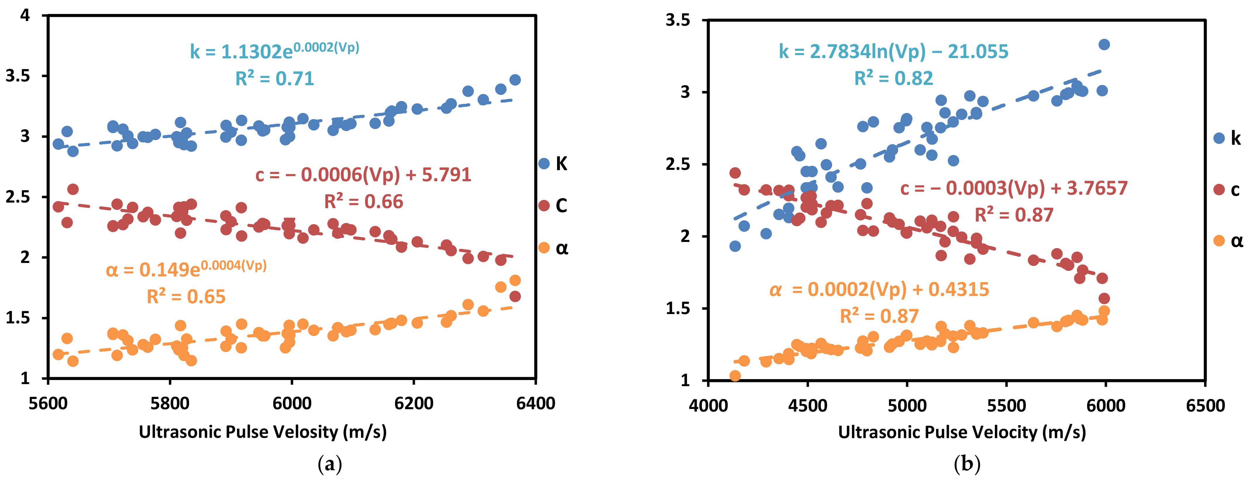
| Vp | m/s | k = 1.1302e0.0002 Vp c = −0.0006 Vp + 5.791 α = 0.149e0.0004 Vp | 0.71 0.66 0.65 | 60 66 63 | 0.64 0.09 0.26 | k = 2.7834ln(Vp) - 21.055 c = −0.0003 Vp + 3.7657 α = 0.0002 Vp + 0.4315 | 0.82 0.87 0.87 | 82 86 85 | 0.13 0.21 0.15 |
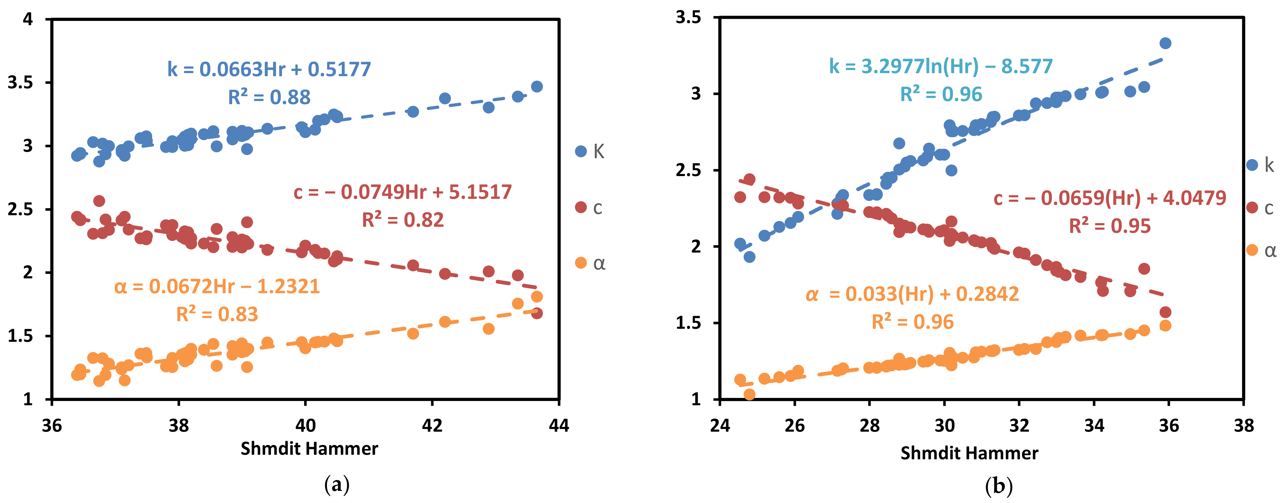
| Hr | - | k = 0.066 Hr + 0.518 c = −0.0749 Hr + 5.151 α = 0.0672 Hr − 1.2321 | 0.88 0.82 0.83 | 88 82 83 | 0.04 0.06 0.05 | k = 3.2977ln(Hr) − 8.577 c = −0.0659 Hr + 4.0479 α = 0.033 Hr + 0.2842 | 0.96 0.95 0.96 | 96 95 96 | 0.06 0.04 0.02 |
| n% | - | k = −0.362ln(n) + 3.5343 c = 0.4067ln(n) + 1.7455 α = −0.361ln(n) + 1.8182 | 0.63 0.58 0.58 | 63 58 58 | 0.07 0.09 0.08 | k = −0.0925 n + 3.3856 c = 0.3897ln(n) + 1.2849 α = −0.0278 n + 1.5022 | 0.90 0.90 0.90 | 90 90 91 | 0.10 0.06 0.02 |
| UCS | MPa | k = 0.0075 UCS + 2.3565 c = −0.0085 UCS + 3.0691 α = 0.0075 UCS + 0.6455 | 0.87 0.80 0.79 | 87 80 79 | 0.04 0.06 0.06 | k = 1.7287ln(UCS) − 4.5797 c = −0.0159 UCS + 3.1098 α = 0.0079 UCS + 0.7577 | 0.87 0.84 0.83 | 88 84 83 | 0.11 0.07 0.04 |
| Is(50) | MPa | k = 0.371 Is(50) + 1.6507 c = −0.4326 Is(50) + 3.9225 α = 0.3852 Is(50) − 0.1196 | 0.82 0.82 0.81 | 82 82 81 | 0.05 0.06 0.05 | k = 0.6825 e0.4718 Is(50) c = −0.6648 Is(50) + 3.96 α = 0.6056 Is(50) 0.7124 | 0.85 0.72 0.72 | 85 72 71 | 0.12 0.09 0.05 |
| Model | R2 | VAF% | RMSE |
|---|---|---|---|
| k = 2.932 − 0.073(n%) + 0.004 (UCS) | 0.94 | 88 | 0.04 |
| α = 6.161 + 0.005 (UCS) − 4.56(Gs)+2.620(ρd) + 0.056 (n%) | 0.80 | 84 | 0.05 |
| c = −13.682+7.60(Gs)+1.932(ρd) − 0.011(UCS) + 0.386 (Is(50)) | 0.69 | 84 | 0.06 |
| DV | Structure | Training Results | Validation Results | ||||
|---|---|---|---|---|---|---|---|
| R2 | MAE | RMSE | R2 | MAE | RMSE | ||
| k | 2-2-1 | 96.07 | 0.050 | 0.065 | 98.03 | 0.032 | 0.041 |
| α | 7-4-1 | 86.7 | 0.036 | 0.048 | 75.70 | 0.023 | 0.039 |
| c | 7-4-2-1 | 92.16 | 0.043 | 0.043 | 92.08 | 0.049 | 0.056 |
Publisher’s Note: MDPI stays neutral with regard to jurisdictional claims in published maps and institutional affiliations. |
© 2022 by the authors. Licensee MDPI, Basel, Switzerland. This article is an open access article distributed under the terms and conditions of the Creative Commons Attribution (CC BY) license (https://creativecommons.org/licenses/by/4.0/).
Share and Cite
Sharo, A.A.; Rabab'ah, S.R.; Taamneh, M.O.; Aldeeky, H.; Al Akhrass, H. Mathematical Modelling for Predicting Thermal Properties of Selected Limestone. Buildings 2022, 12, 2063. https://doi.org/10.3390/buildings12122063
Sharo AA, Rabab'ah SR, Taamneh MO, Aldeeky H, Al Akhrass H. Mathematical Modelling for Predicting Thermal Properties of Selected Limestone. Buildings. 2022; 12(12):2063. https://doi.org/10.3390/buildings12122063
Chicago/Turabian StyleSharo, Abdulla A., Samer R. Rabab'ah, Mohammad O. Taamneh, Hussein Aldeeky, and Haneen Al Akhrass. 2022. "Mathematical Modelling for Predicting Thermal Properties of Selected Limestone" Buildings 12, no. 12: 2063. https://doi.org/10.3390/buildings12122063
APA StyleSharo, A. A., Rabab'ah, S. R., Taamneh, M. O., Aldeeky, H., & Al Akhrass, H. (2022). Mathematical Modelling for Predicting Thermal Properties of Selected Limestone. Buildings, 12(12), 2063. https://doi.org/10.3390/buildings12122063