1. Introduction
During the last few decades, due to its application in several areas in science and engineering, the study of flow and heat transfer over an unsteady stretching sheet has drawn significant attention to researchers. The study of rotating flow and heat transfer has received fervent interest in modern fluid dynamics research, with applications in geophysics, biomedical engineering, medical science, planetary science, thermal insulations, etc.
Biomagnetic Fluid Dynamics (BFD) is the study of the effects of an applied magnetic field on biological fluid flow [
1]. The most characteristic biomagnetic fluid is blood. Blood is a suspension of numerous cells such as red blood cells, white blood cells, and platelets in a liquid electrolyte solution called plasma. Plasma contains 7% of principal proteins and 90% of water, along with considerable concentration of ions. Blood as a whole is considered as a non-Newtonian fluid predominantly when the characteristic dimension of the flow is nearby the cell dimension. As far as the stretching sheet flows are concerned, Crane [
2] computed an exact similarity solution for the boundary layer flow of a Newtonian fluid towards an elastic sheet. The sheet was stretched with the velocity proportional to the distance from the origin. Barozzi and Dumas [
3] numerically studied the convective heat transfer in blood vessels of the circulatory system. They observed that the rheological behavior of blood does not significantly affect the heat transfer rate in small blood vessels. Pennes [
4] studied the effects of blood perfusion and metabolic heat generation in living tissues using a simplified bio-heat transfer model. Although this model bears the potential to describe the effect of blood flow on tissue temperature, it has some considerable short comings. This is because uniform perfusion rate was assumed, and the direction of blood flow was not accounted for. Moreover, in his model, only the stream of venous blood as the fluid stream equilibrated with tissue was considered.
In recent years, the study of the magneto hydrodynamic (MHD) flow of blood through the arteries has gained considerable interest because of its important applications in physiology. Theoretical estimates of blood flow in arteries during the therapeutic procedure of electromagnetic hyperthermia used for cancer treatment were reported by Misra et al. [
5]. A few important discussions were also available in that paper. The effects of electromagnetic radiation/ultrasonic radiation on blood flow were studied by other investigations such as those of Inoue et al. [
6], Nishimoto et al. [
7], Bidin and Nazar [
8], Irfan et al. [
9], and Ishak [
10]. The effect of viscous dissipation and radiation on the unsteady flow of electrically conducting fluid passed over a stretching surface was considered by Brickman [
11] and Chand et al. [
12]. The variable viscosity and thermal conductivity effects of combined heat and mass transfer in mixed convection over a UHF/UMF wedge in porous media were analyzed by Hassanien et al. [
13] and Khan et al. [
14]. Moreover, the effects of variable viscosity and thermal conductivity on a thin film flow over a shrinking/stretching sheet were also studied. Pal and Mondal [
15] studied the effects of temperature-dependent viscosity and variable thermal conductivity on an MHD, non-Darcy mixed convection diffusion of species over a stretching sheet. The effects of thermal radiation over a stretching sheet under several flow conditions have been also studied by several researchers [
16,
17,
18,
19,
20].
Furthermore, a study of microploar fluid under the influence of a magnetic field through a stretched curved surface, using the Cattaneo–Christov heat model investigated by Khan et al. [
21], had found that, in fluid velocity, the magnetic field parameter plays a significant role. The movement of peristaltic flow of a dusty fluid with elastic properties in a curved configuration was analyzed by Khan et al. [
22]. A fully developed model of non-Newtonian fluid through a 2D stretching sheet in the presence of Lorentz force and internal heat was presented by Vijaya et al. [
23]. The BFD model [
1], which involves both ferrohydrodynamics (FHD) and magnetohydrodynamics (MHD) principles, was utilized for the study of the effect of thermal radiation through a two-dimensional unsteady stretching sheet by Alam et al. [
24]. Finally, the impact of MHD on non-Newtonian mass and heat transfer along a curved stretched sheet was numerically studied by Yasim et al. [
25].
The aim of the present investigation is to study the flow and heat transfer in a stretching sheet with an angle
to the vertical plane in the presence of a non-uniform source/sink. The mathematical formulation of the effect of the magnetic field is that of BFD, involving both principles of ferrohydrodynamics (FHD) and MHD [
1]. The governing partial differential equations have been transformed by similarity transformations into a coupled system of nonlinear ordinary differential equations. The solution was attained by using a MATLAB package. The effects of various parameters on the momentum and heat transfer characteristics have been studied, and the numerical results are presented graphically for the various values of the parameters entering the problem into consideration.
2. Model Description
The unsteady two-dimensional BFD flow of a viscous incompressible fluid past a stretching sheet with an acute angle to the vertical is considered.
Where
and
are the velocity components along
-direction and
-direction, respectively. The
-axis is considered along the plate and
-axis is taken normal to it (see
Figure 1). Initially
, the sheet is stretched with velocity
along the
-axis, whereas the origin is kept fixed in the fluid medium of ambient temperature
, and
is the stretching surface temperature. A magnetic field of uniform strength
is acting normal to the direction of the flow, with an acute angle
. The magnetic Reynold’s number is assumed as much less than unity, and the flow is considered two-dimensional, therefore the induced magnetic field can be neglected in comparison to the applied magnetic field. Moreover, the fluids exhibit polarization due to the incorporated principles of FHD, and the applied magnetic field is assumed to be strong enough to attain equilibrium magnetization. The velocity slip, thermal slip, viscous dissipation parameter, and ferromagnetic interaction parameter have been taken into account. The boundary layer equations of the fluid and energy equation for the problem can be written as [
1,
26,
27].
Energy (Heat) conservation:
Here, is the biomagnetic fluid density, , where is a constant representing the magnetic field strength at is the time dependent permeability parameter, is the constant permeability of the medium, is the acceleration due to gravity, is the coefficient of thermal expansion, is the thermal conductivity, is the specific heat at constant pressure, is the kinematic coefficient of viscosity, is the electrical conductivity, is the radiative heat flux, is the magnetization, is the magnetic field of the fluid, and is the temperature of the field.
The boundary conditions for the problem can be written as: [
27,
28]
Here, is the stretching velocity, is the surface temperature. Where are the constants such that and .
In Equation (4),
represents the blood velocity at the wall and is equal to injection/suction velocity given by
As it is implied by Equation (5), the mass transfer at the sheet of the wall takes place with a velocity . For the case of injection, it is considered that , whereas is considered for the case of suction. is the velocity slip factor, is the coefficient of viscosity, is the thermal slip factor. The no-slip conditions hold when .
Using the Rosseland approximation [
27], the radiation heat flux
is simplified as
where
and
are the Stefan–Boltzman constant and the mean absorption co-efficient, respectively.
Considering that the temperature differences within the flow are such that the term
may be expressed as a linear function of the temperature,
is expanded in a Taylor series about
. By neglecting the higher order terms beyond the first degree in
, it is obtained that
The non-uniform heat source/sink
is defined as
where
and
are the coefficient of a space- and temperature-dependent heat source/sink, respectively. The case of
corresponds to internal heat generation, and that of
corresponds to internal heat absorption. Physically, the role of a heat source in a fluid transport is to enhance its thermal conductivity, which consequently results in increased fluid temperature. On the other hand, heat sink decreases the thermal conductivity, which results in a decrease in the temperature of the fluid.
By substituting (5) and (6) into (3), the energy equation is reduced to
The term
in Equation (2) denotes the component of magnetic force per unit volume. This term is heavily dependent on the presence of a magnetic gradient, and, when the magnetic gradient is absent, this force vanishes. The heating due to adiabatic magnetization is represented by the second term, on the left hand side of the thermal energy Equation (8). The components
and
of the magnetic field
, which are due to a magnetic dipole, are given by [
29,
30]
where
is a scalar potential of the magnetic dipole,
and
is a dimensionless distance defined as
.
Thus, the magnetic field strength intensity
is given by
The corresponding gradients are given by
The magnetization
is generally determined by the fluid temperature provided that the applied magnetic field
is sufficiently strong enough to saturate the biomagnetic fluid. Anderson and Valnes [
29] considered that the variation of magnetization
with temperature
can be approximated by the linear equation
where
is a constant.
To transform the momentum and energy equations, the following transformations are defined:
Here, is the similarity variable, is the stream function, and are dimensionless quantities.
The continuity Equation (1) is satisfied by the stream function
as
and
Making use of Equation (9), Equations (2) and (8) can be written as
The boundary conditions are transformed to:
In Equation (12), and correspond to injection and suction, respectively. In the equation written above, primes denote derivatives with respect to . and are the non-dimensional velocity slip factor and thermal slip factor, respectively.
Furthermore, is the unsteadiness parameter, is the Prandtl number, is the viscous dissipation parameter, is the dimensionless curie temperature, is the ferromagnetic interaction parameter, is the permeability parameter, is the magnetic field parameter, is the radiation parameter, is the Grashof number, is the Eckert number, is the dimensionless distance, and is the local Reynolds number.
The skin friction coefficient and the Nusselt number constitute important characteristics of the flow, defined as:
where, the wall stress
and the heat transfer
from the sheet are given by
Using the similarity variables (9), it is obtained that:
4. Parameter Estimation
In this study, the unsteady biomagnetic fluid flow along a two-dimensional stretching/shrinking sheet under the action of a magnetic field is investigated numerically. In order to achieve the numerical solution, it is necessary to determine some specific values for the dimensionless parameters, such as the Prandtl number, the unsteadiness parameter, the magnetic field parameter, the permeability parameter, the radiation parameter, the ferromagnetic interaction parameter, the Grashof number, the Eckert number, the suction/injection parameter, the non-dimensional velocity-slip factor, the non-dimensional thermal slip factor, the acute angle of magnetic field, the inclination angle, the co-efficient of space and temperature.
Many researchers have, in scientific literatures, reported various values of the abovementioned dimensionless parameters. It is understood that, for human blood, the following data are considered:
in [
31,
32,
33], where, human body temperature is considered to be
°C and the body Curie temperature is considered to be
°C. For this value of temperature, the dimensionless temperature is
.
Using these values, we have .
That is, for human blood flow, the Prandtl number is 21.
For the results presented in the following Figures 2–39, we consider the values of the dimensionless parameters entering into the problem under consideration as follows:
- (1)
Unsteadiness parameter
as in [
34]
- (2)
Radiation parameter
as in [
24,
28,
35,
36]
- (3)
Prandtl number
as in [
29,
37,
38]
- (4)
Ferromagnetic interaction parameter
as in [
30,
37,
38]
- (5)
Dimensionless distance
as in [
34,
36,
38]
- (6)
Viscous dissipation parameter
as in [
24,
37,
38]
- (7)
Dimensionless curie temperature
as in [
29,
37,
38]
- (8)
Suction/injection parameter
as in [
20,
27]
- (9)
Magnetic field parameter
as in [
24,
31,
38]
- (10)
Permeability parameter
as in [
27,
31]
- (11)
Eckert number
as in [
27,
31,
37,
38]
- (12)
Grashof number
as in [
27,
31]
- (13)
Non-dimensional velocity-slip factor
as in [
27,
31]
- (14)
Non-dimensional thermal slip factor
as in [
27,
31]
- (15)
Acute angle of magnetic field
as in [
27,
31,
34]
- (16)
Inclination angle
as in [
27,
31]
- (17)
Co-efficient of space
as in [
27,
31]
- (18)
Co-efficient of temperature
as in [
27,
31]
5. Results and Discussion
In order to assess the validity of the numerical results, the values of local Nusselt number
have been compared with the existing works of Magyari and Keller [
35], El-Aziz [
36], Bidin and Nazar [
8], and Anwar Ishak [
10] by setting
. It is apparent from the
Table 1 that the numerical scheme and the coding used give results in good agreement with the abovementioned, previously published studies.
A comparison of the local Nusselt number for various values .
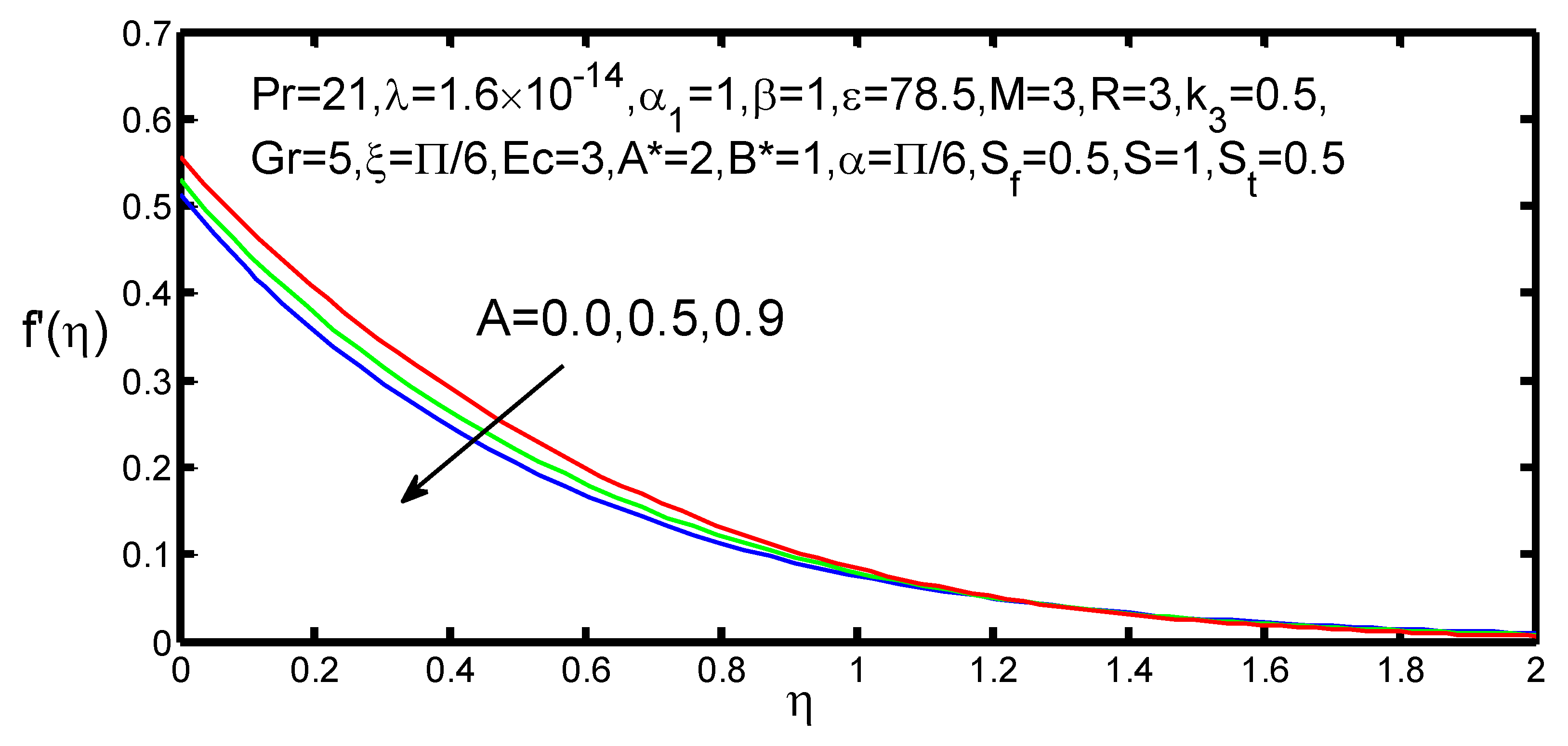
Figure 2 and
Figure 3 show the velocity and temperature distributions with various values of the unsteadiness parameter
. From
Figure 2, it is observed that the velocity profiles are decreased as the unsteadiness parameter is increasing. This is justified because the accompanying reduction in the thickness of the momentum in the boundary layer. Moreover, from
Figure 3, it is obtained that the temperature profiles are decreased significantly as the unsteadiness parameter is increased. The fact is that, when the unsteadiness parameter is increased, less heat is transferred from the sheet to the fluid.
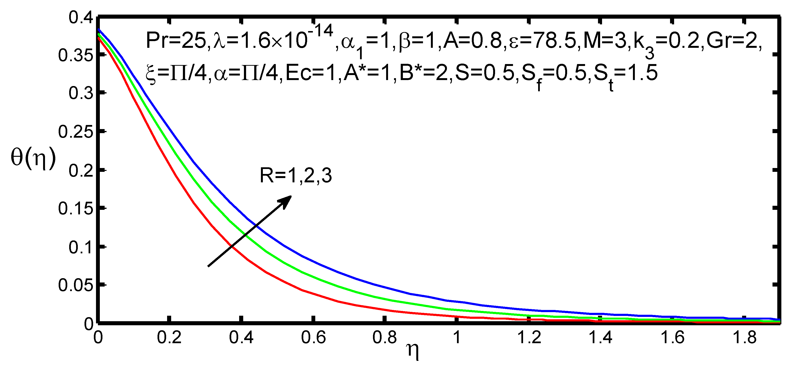
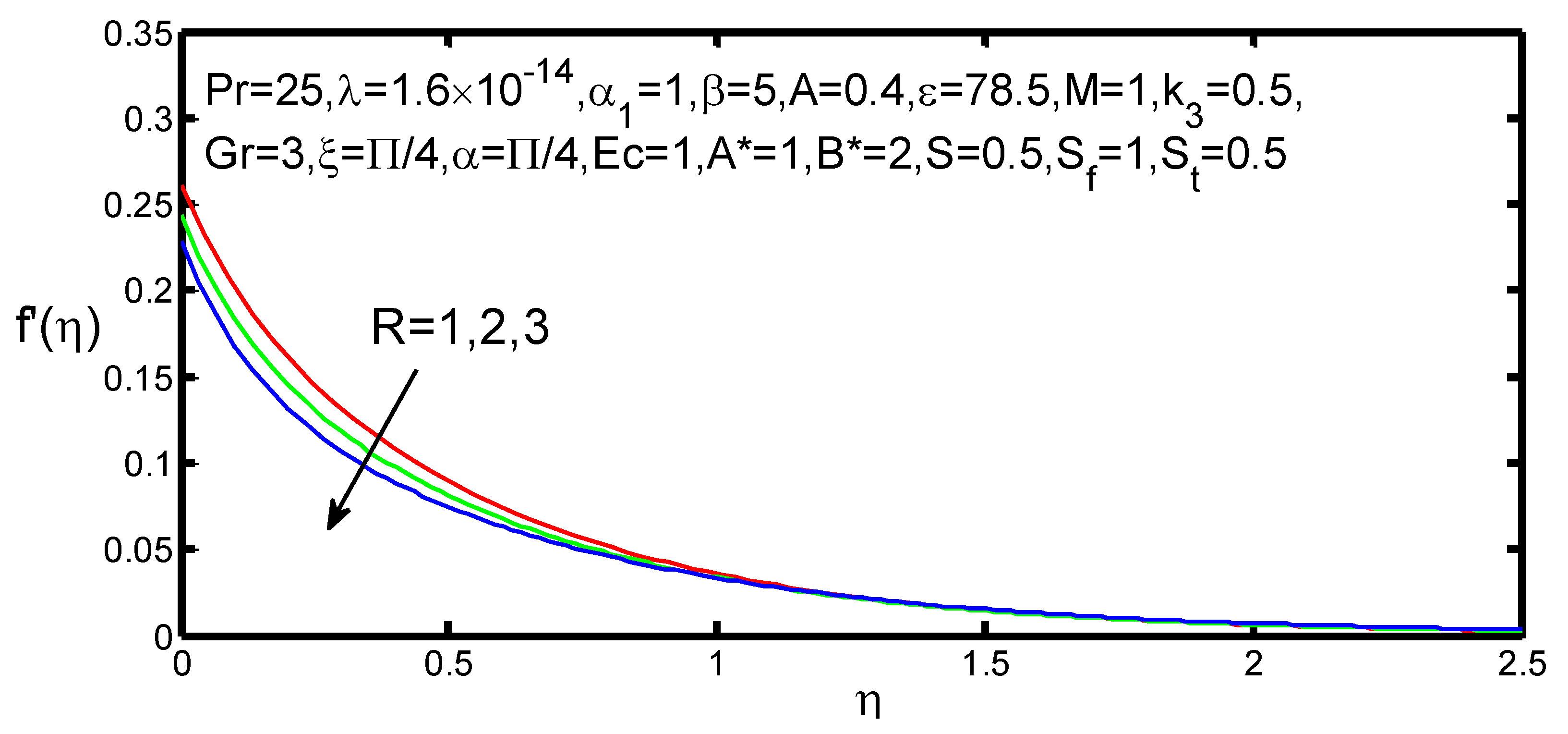
Figure 4 and
Figure 5 show the velocity and temperature profiles for various values of the radiation parameter
. From
Figure 4 and
Figure 5, it is observed that an increment in radiation parameter
results in a decrement in the fluid velocity profile, whereas the temperature profile increases. The temperature profile is increased because the effect of the radiation parameter is to enhance heat transfer. The thermal boundary layer thickness is increased with the increment of the thermal radiation.
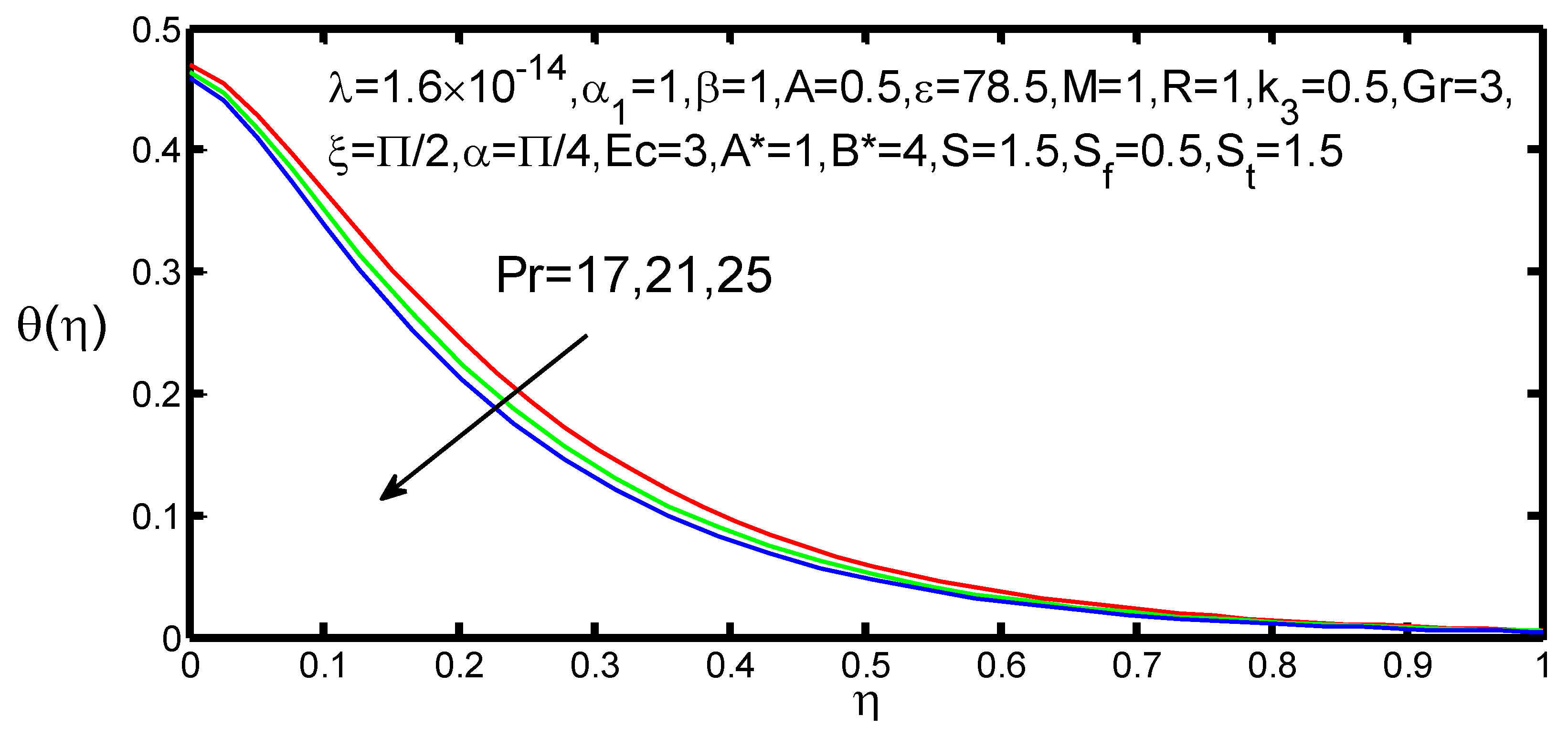
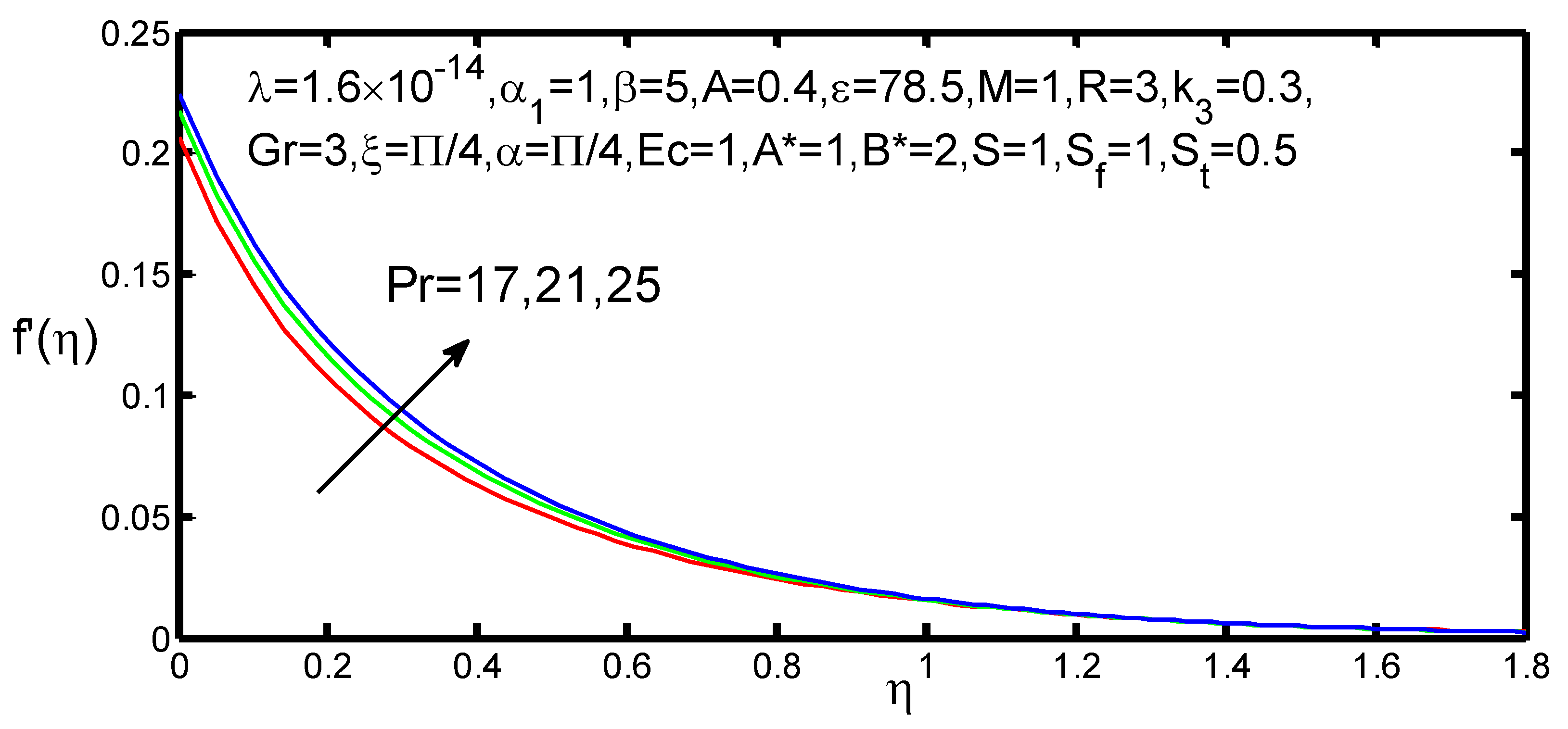
The velocity and temperature profiles with various values of Prandtl number
are shown in
Figure 6 and
Figure 7. It is observed that an increment in
causes an increment in the velocity profile, whereas the temperature profile is decreased. This occurs because an increment in the Prandtl number means a decrement in the thermal diffusivity, and this phenomenon leads to the decreasing of energy ability that finally results in the reduction of the thermal boundary layer thickness.
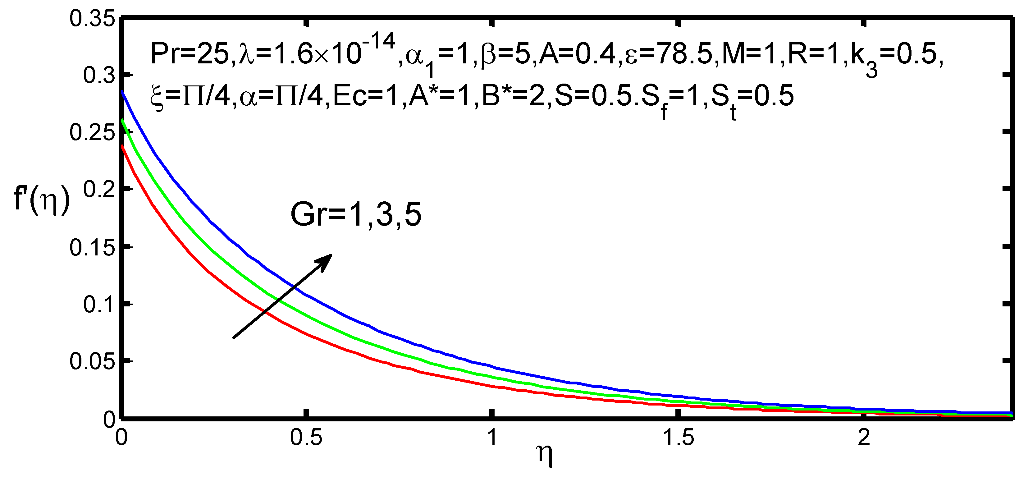
Figure 8 and
Figure 9 show the effect of the Grashof number
on the profiles of velocity and temperature. It was found that, with an increment in the Grashof number, which increases the velocity profile, the opposite is true for the temperature profile. This is due to the fact that an increase in the Grashof number means increment of the buoyancy forces which finally reduce the thermal boundary layer thickness.
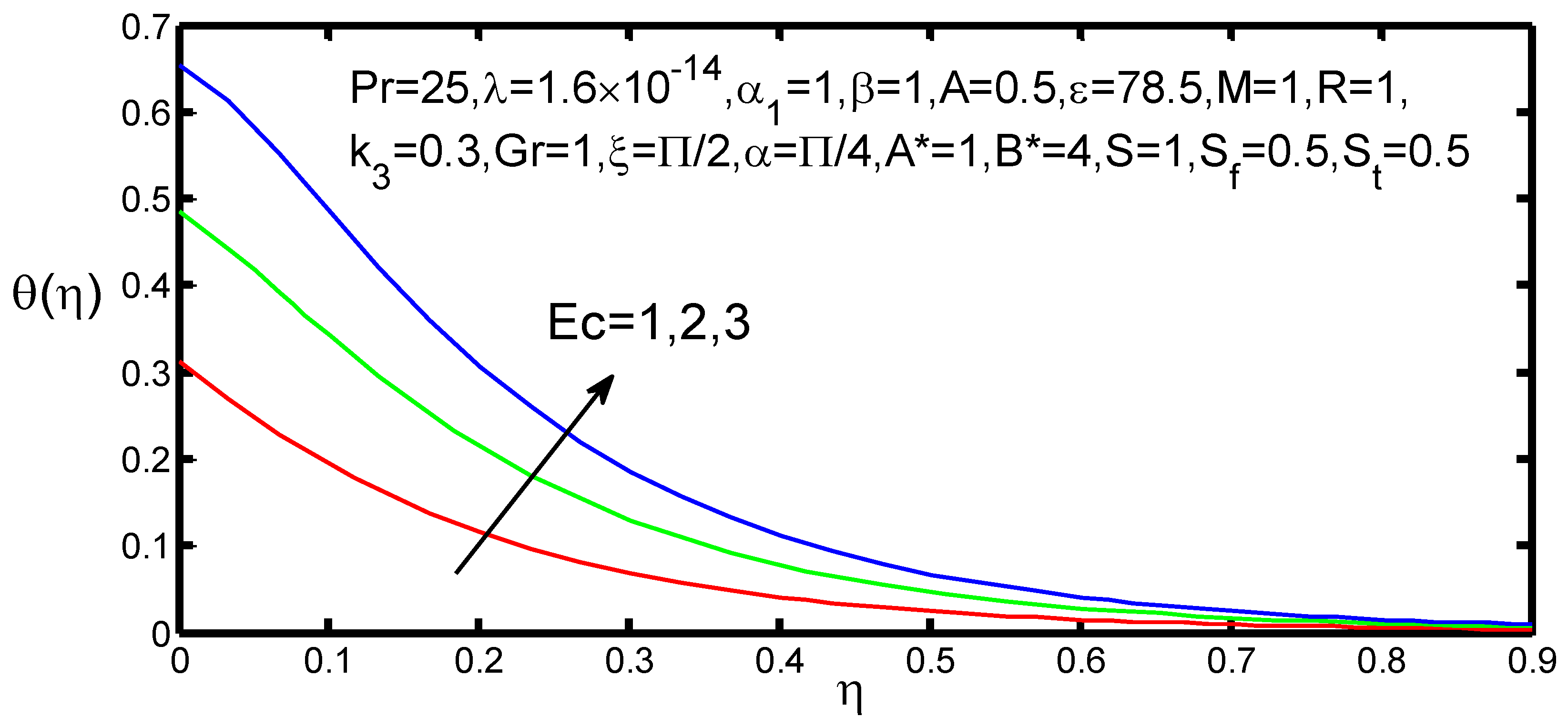
The velocity and temperature profiles for various values of the Eckert number
are shown in
Figure 10 and
Figure 11. The relationship between the kinetic energy in the flow and the enthalpy is expressed by the Eckert number. It assimilates the conversion of kinetic energy into internal energy by the work done against the viscous fluid stresses. The positive Eckert number implies cooling of the sheet. Hence, greater viscous dissipative heat causes a rise in temperature as well as the velocity, both of which are evident in
Figure 10 and
Figure 11.
Figure 12 and
Figure 13 show the effect of the suction/injection parameter
on the velocity and temperature profiles. From the figures, it is observed that the momentum boundary layer thickness is decreased with increasing values of
. It is expected that the increment of the suction results in the decrement of the thickness of the hydrodynamic boundary layer. It also illustrates that an increment in
decreases the temperature profiles in the flow region. This is due to the fact that, as the suction is increased, more warm fluid is taken away from the fluid region, causing a reduction in the thermal boundary layer thickness.
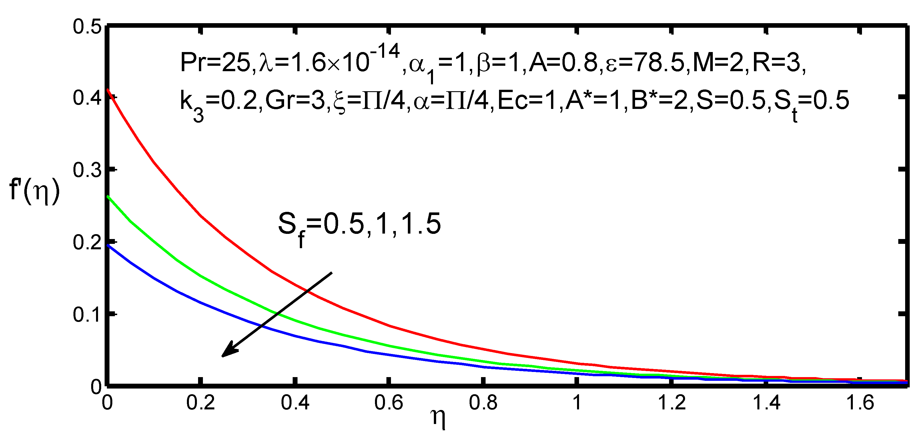
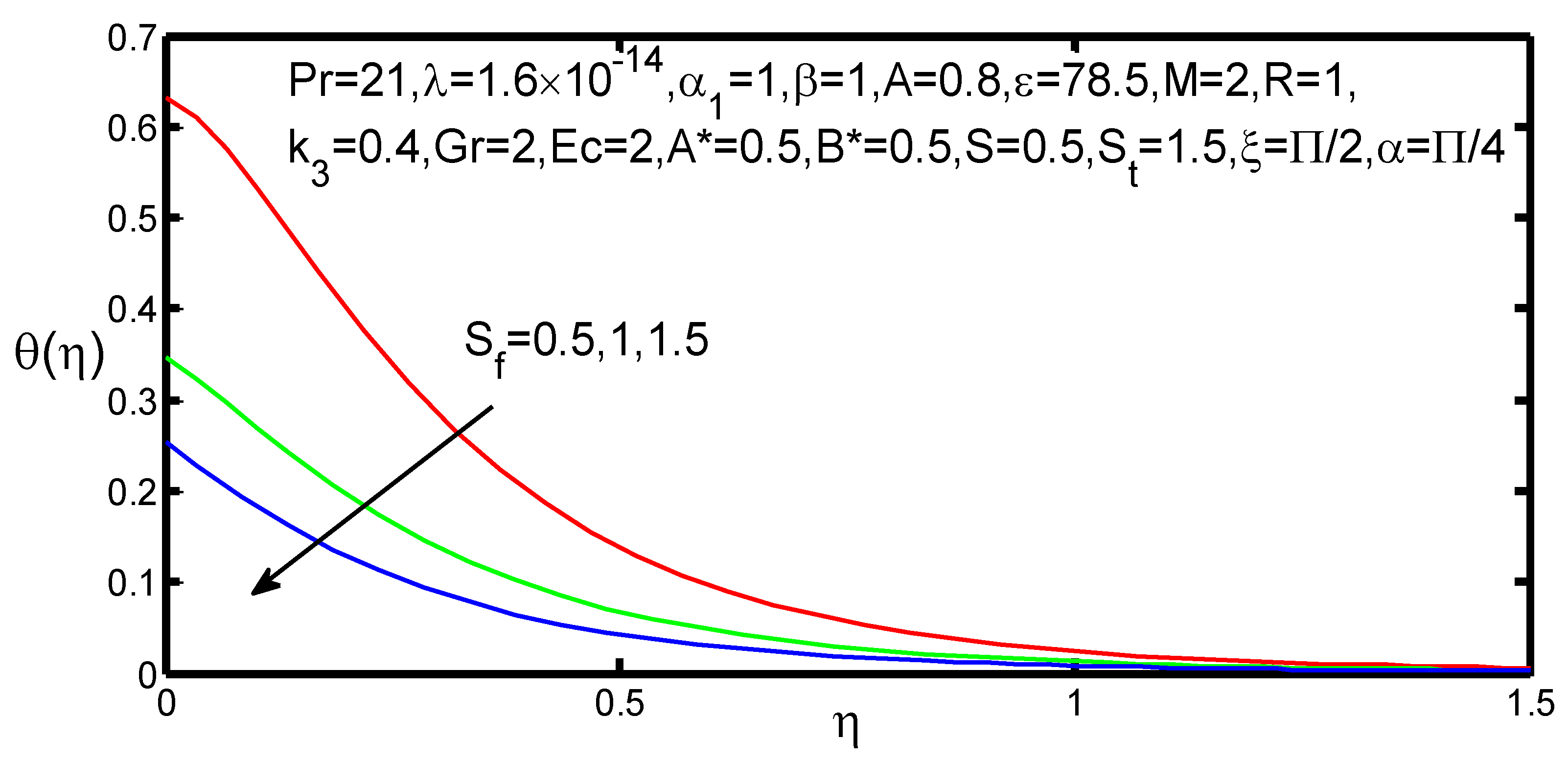
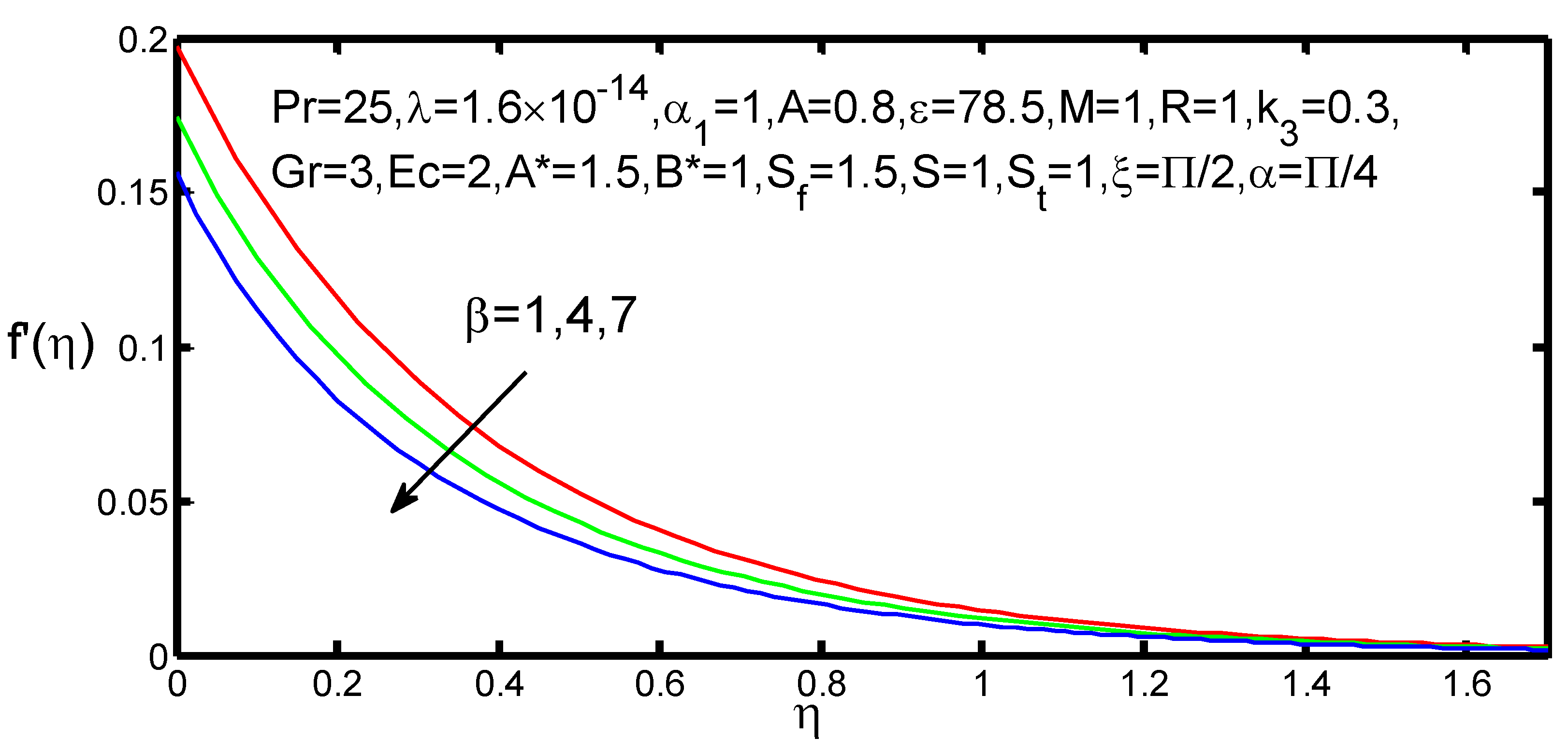
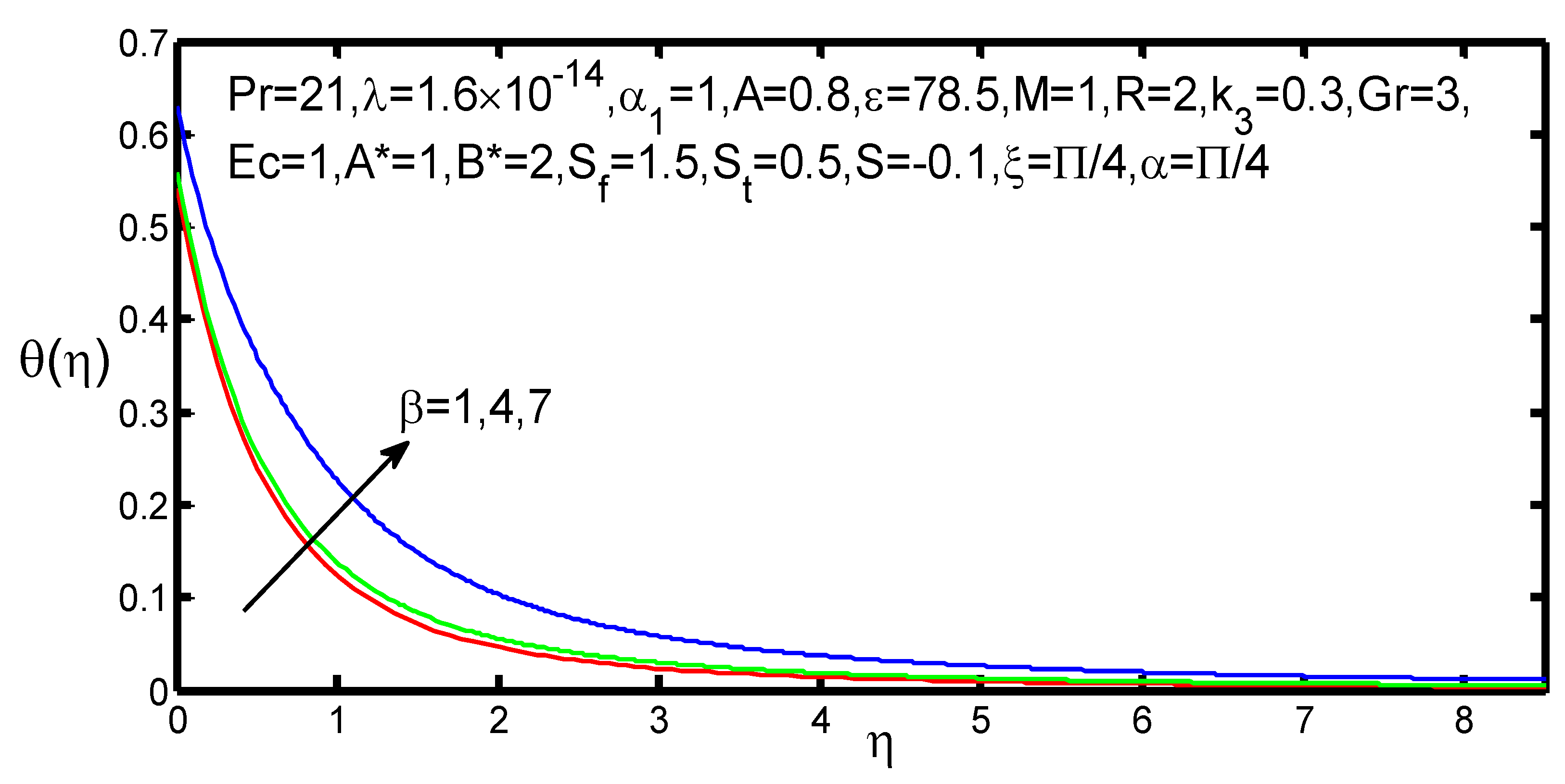
Figure 14 and
Figure 15 show the effect of velocity slip parameter
on the velocity and temperature profiles. From the
Figure 14, it is observed that the presence of velocity slip within the boundary layer causes the velocity level along the sheet to decrease. This is happening because the quantity
increases monotonically with
. We also observe that the temperature profile decreases, as shown in
Figure 15.
The effect of the thermal slip parameter
on the velocity and temperature profiles is shown in
Figure 16 and
Figure 17. In
Figure 16, it can be observed that the presence of the thermal slip factor on the temperature profiles has a significant effect. It is clear that the temperature near the surface is decreased as the values of
are increased. This is happening because the increment in the thermal slip parameter results in the increment of the thermal coefficient, and the thermal diffusion towards the blood flow is reduced. The reverse behavior takes place for the velocity boundary layer, as shown in
Figure 16.
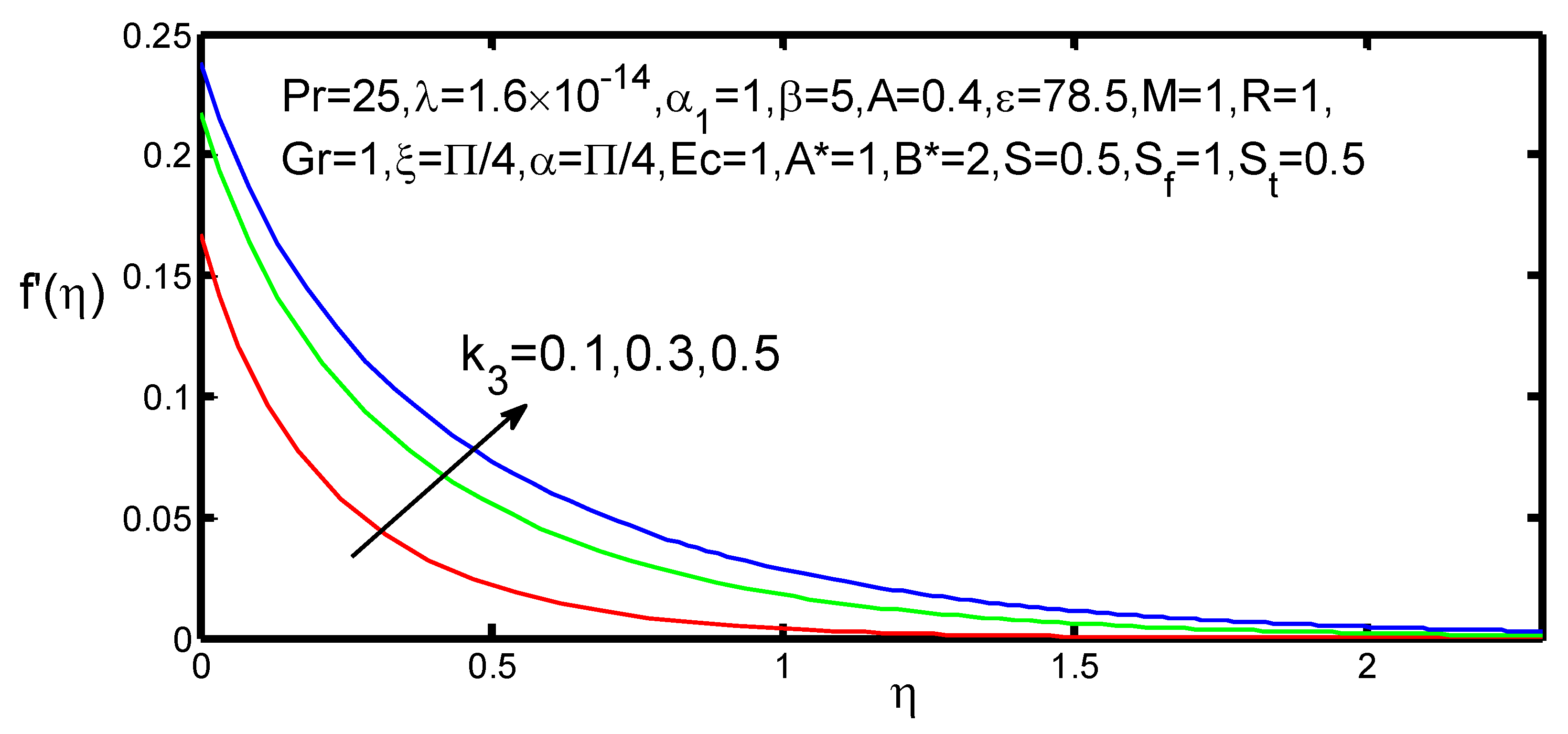
Figure 18 and
Figure 19 show the effects of the permeability parameter
on the velocity and temperature profiles. It is observed from
Figure 18 that the presence of permeability parameter
on the velocity profiles has a significant incremental effect. This is happening because the flow increases over the sheet as the permeability parameter is increased. The resistance on the flow above the sheet is decreased as the permeability of the sheet increases. From
Figure 19, it can be noticed that the temperature profile declines when the permeability parameter
enhances.
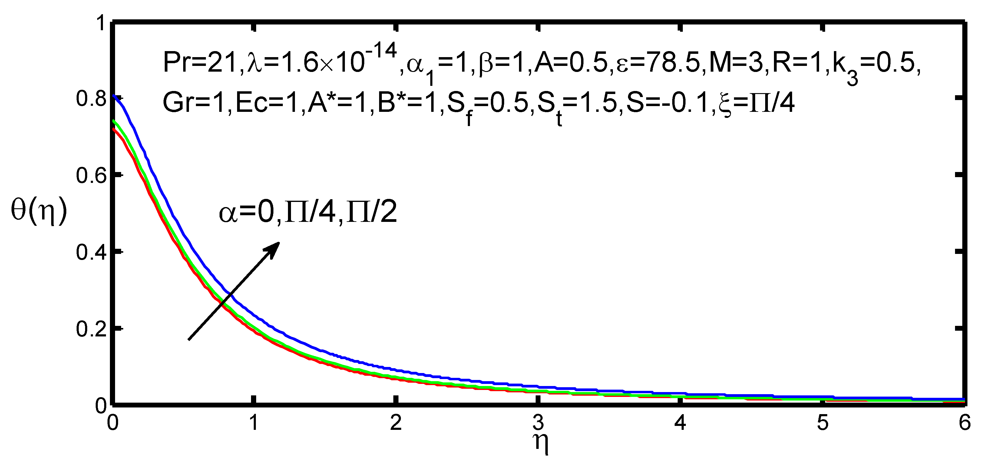
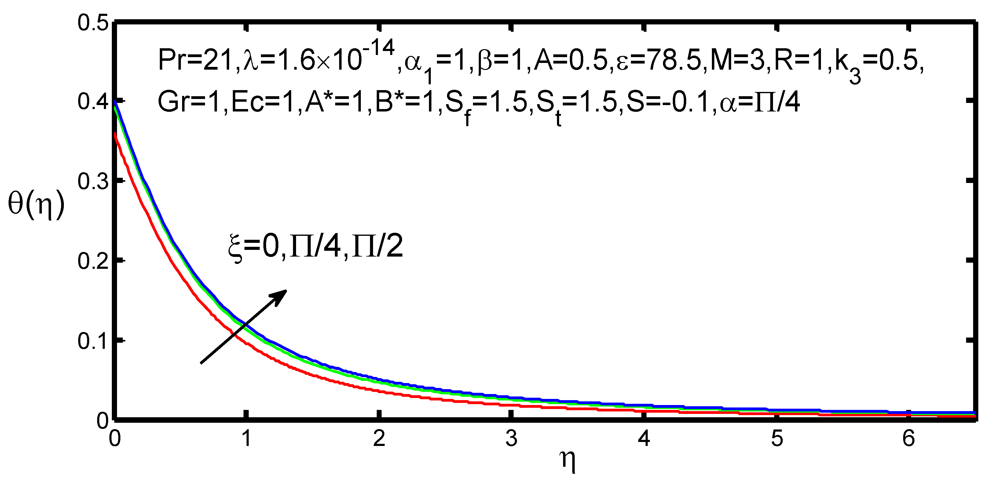
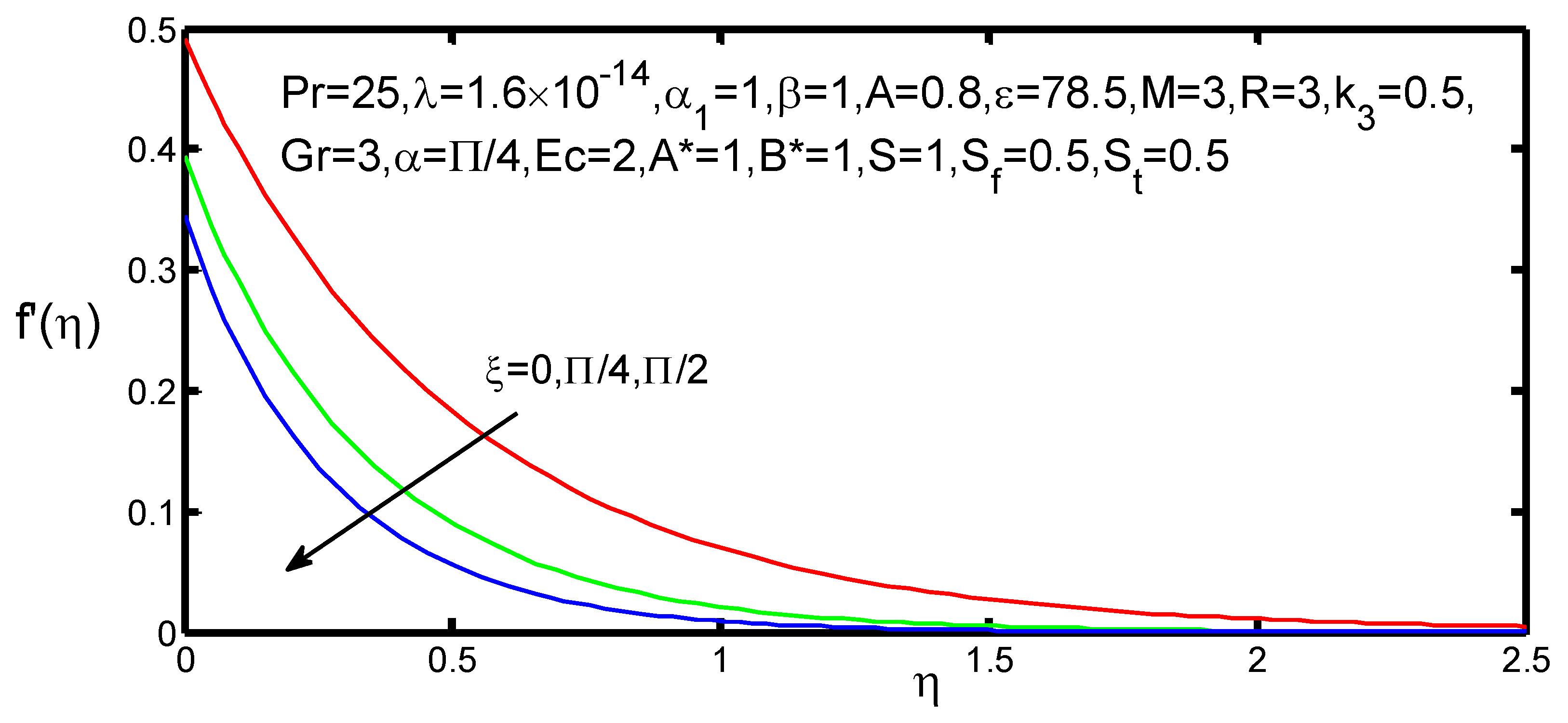
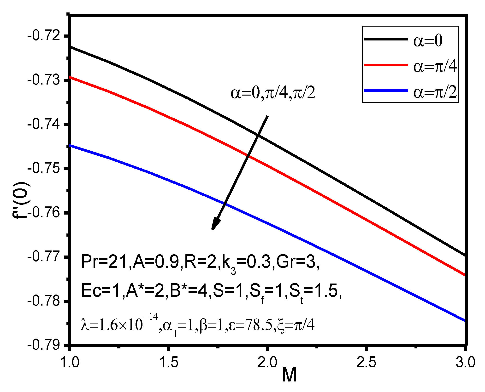
Figure 20 and
Figure 21 show the effect of inclination parameter
on the velocity and temperature profiles. From
Figure 20, we observe that the velocity profile decreases with an increment in the inclination parameter
. It seems that the angle of inclination decreases the effect of the buoyancy force due to thermal diffusion by a factor of
. Therefore, the driving force to the fluid decreases, and, as a result, the velocity is finally decreased. The reverse is happening in the temperature profile, which is shown in
Figure 21.
Figure 22 and
Figure 23 show the effect of the inclination angle of the magnetic field
on the velocity and temperature profiles. It is noticed that the velocity profile is reduced and that the temperature profile is enhanced by the increment in the inclination angle. This may be due to the fact that a rise in the aligned angle makes the applied magnetic field stronger.
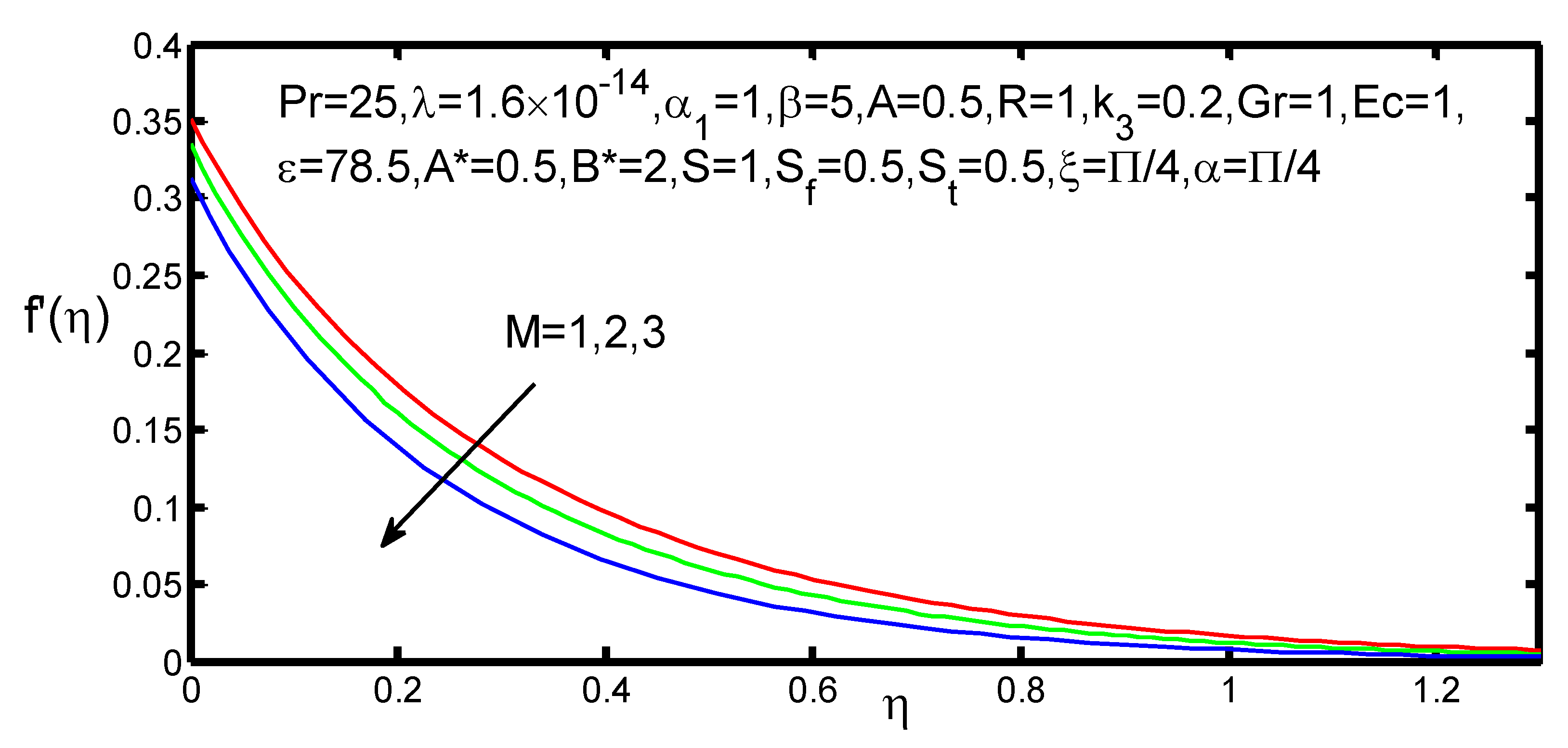
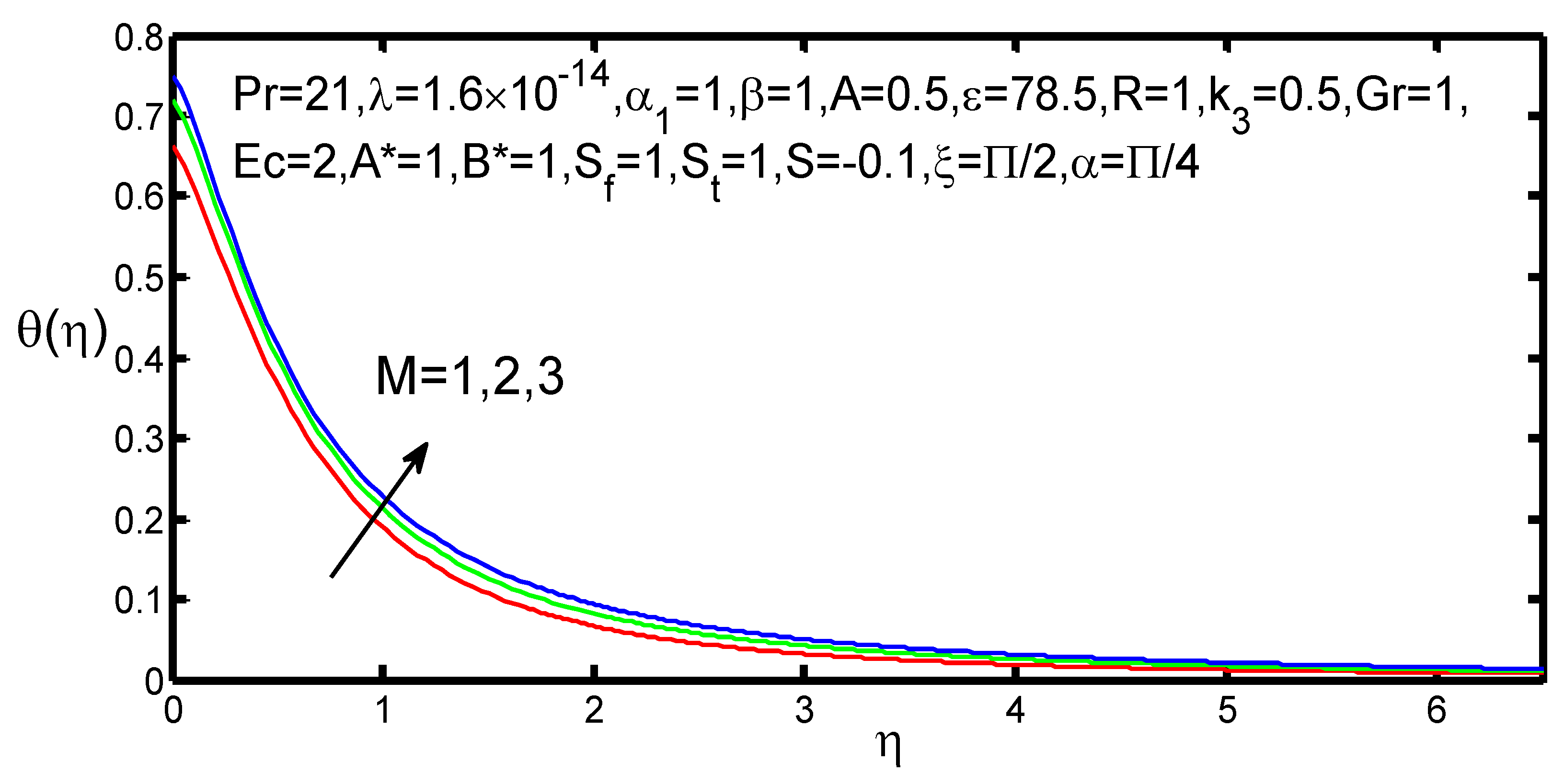
Figure 24 and
Figure 25 depict the effects of the magnetic parameter
on the velocity and temperature profiles. It is observed that the velocity profile is decreased as the magnetic parameter is increased. The increment of the magnetic parameter increases the introduced Lorentz force in the boundary layer, and, hence, the velocity profile in the boundary layer is decreased. An increment in the magnetic parameter would enhance the Lorentz force and, consequently, an augmentation of the Lorentz force opposes the flow, and the fluid motion is reduced. From
Figure 25, it is noticed that the temperature profiles increase as the magnetic parameter increases. This indicates the fact that the introduction of the transverse magnetic field to an electrically conductive fluid gives rise to the Lorentz force. All these effects result in the increment of the temperature of the fluid.
The velocity and temperatre profiles for various values of ferromagnetic interaction parameter
are shown in
Figure 26 and
Figure 27. It is observed that the velocity of the fluid decreases with an increment of ferromagnetic number, whereas the temperature profile is increased in these cases. The region behind that ferromagnetic number is directly related to the celvin force, which is also known as the drug force. The results observed in
Figure 24,
Figure 25,
Figure 26 and
Figure 27 are in accordance with those presented in [
30,
31].
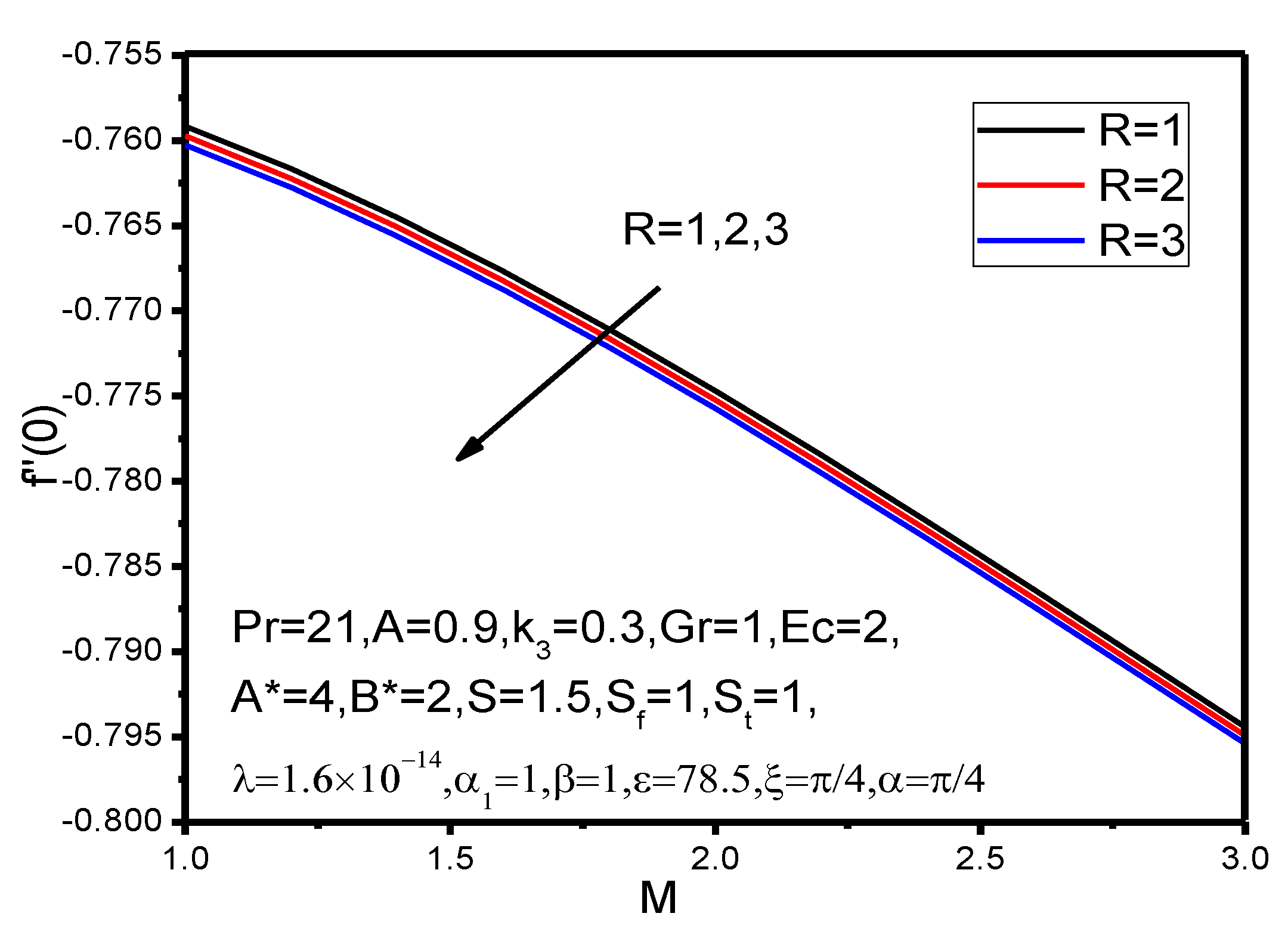
Figure 28,
Figure 29,
Figure 30,
Figure 31,
Figure 32,
Figure 33,
Figure 34,
Figure 35,
Figure 36,
Figure 37,
Figure 38 and
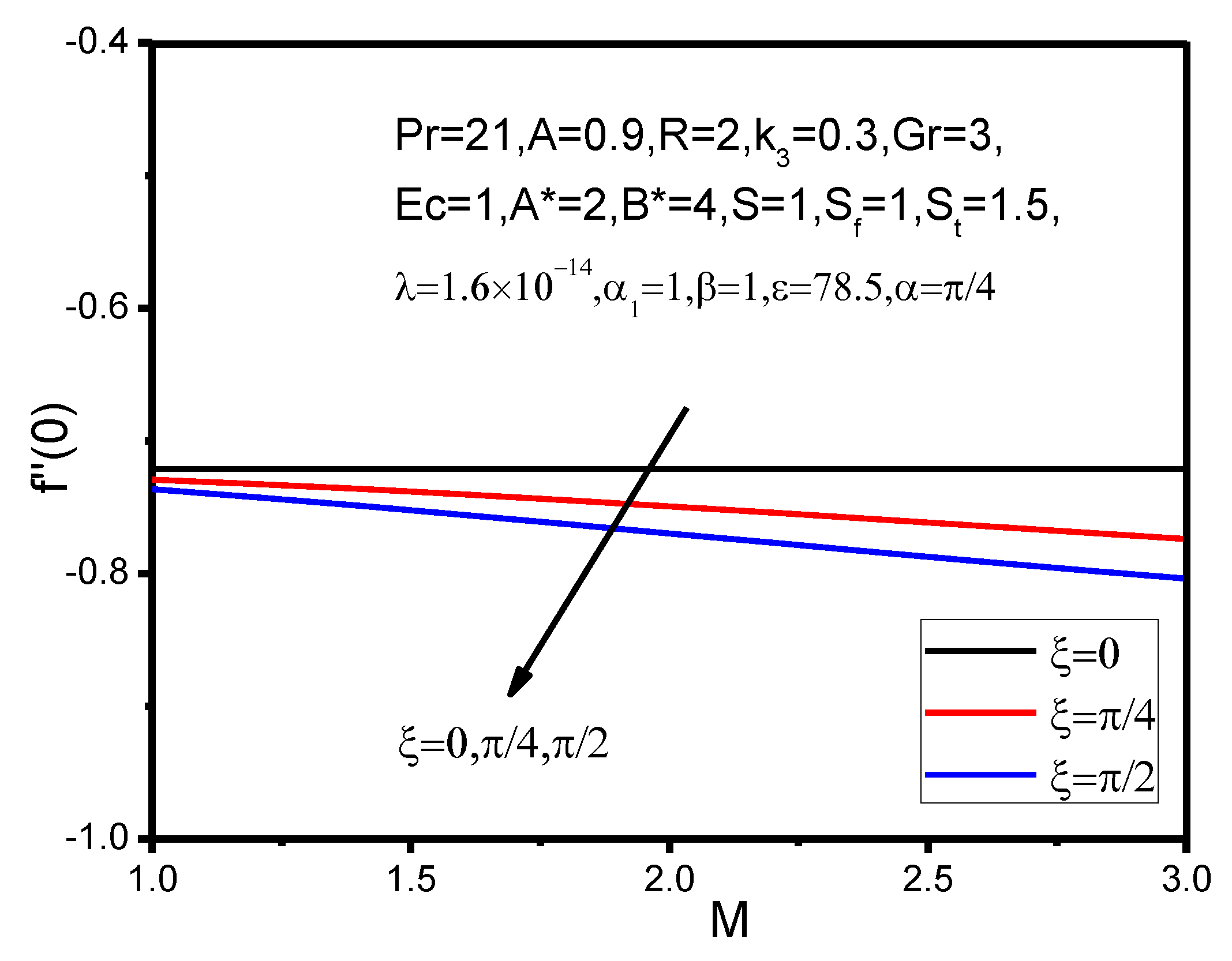
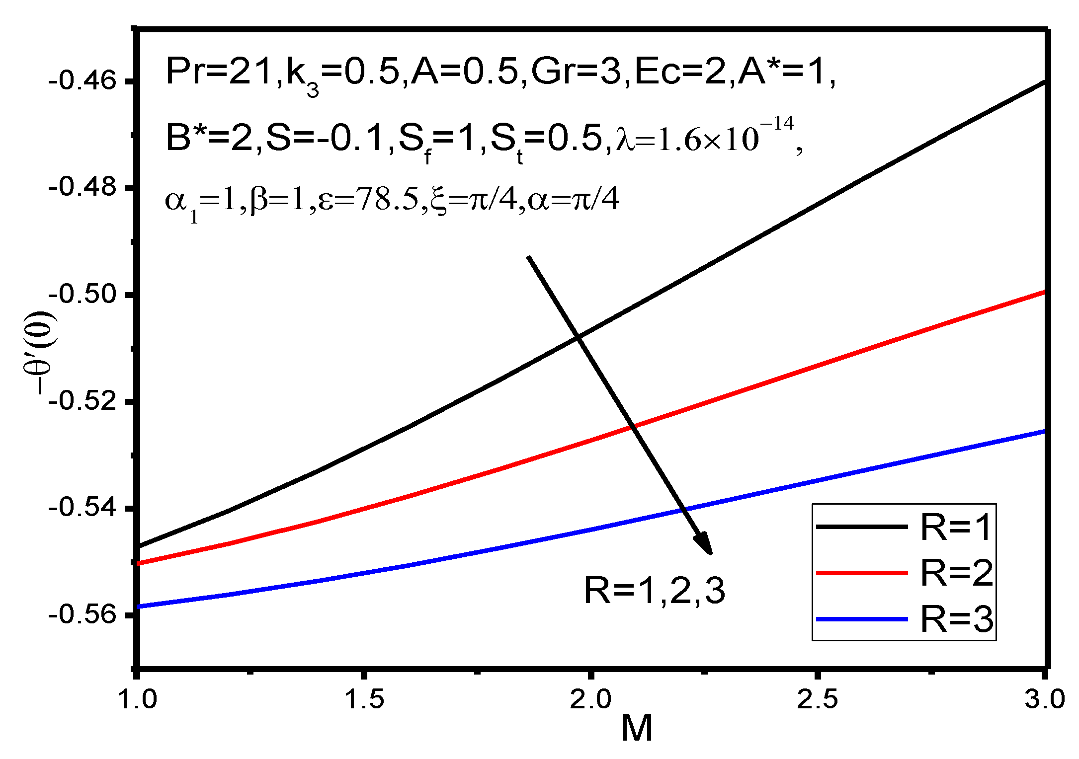
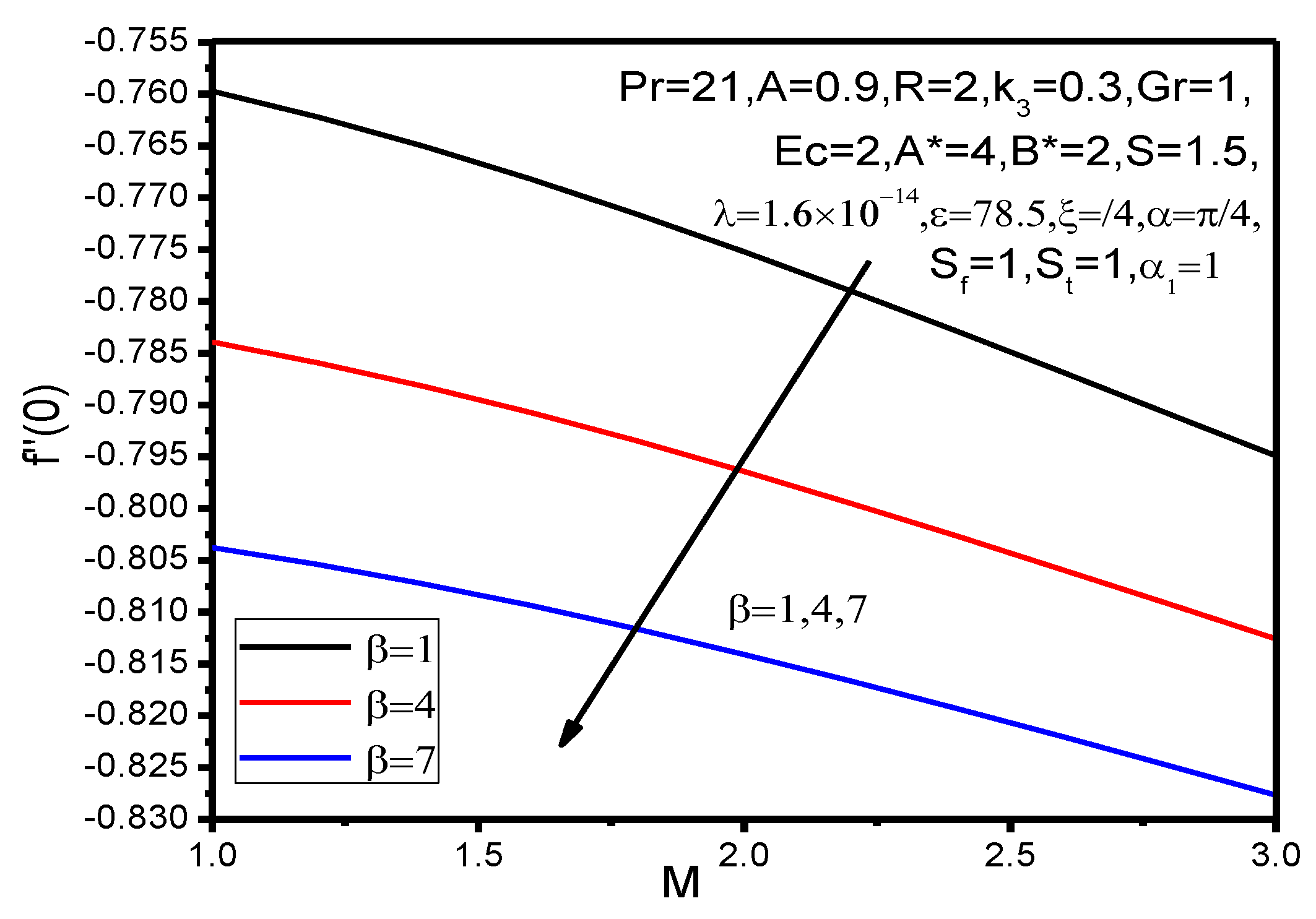
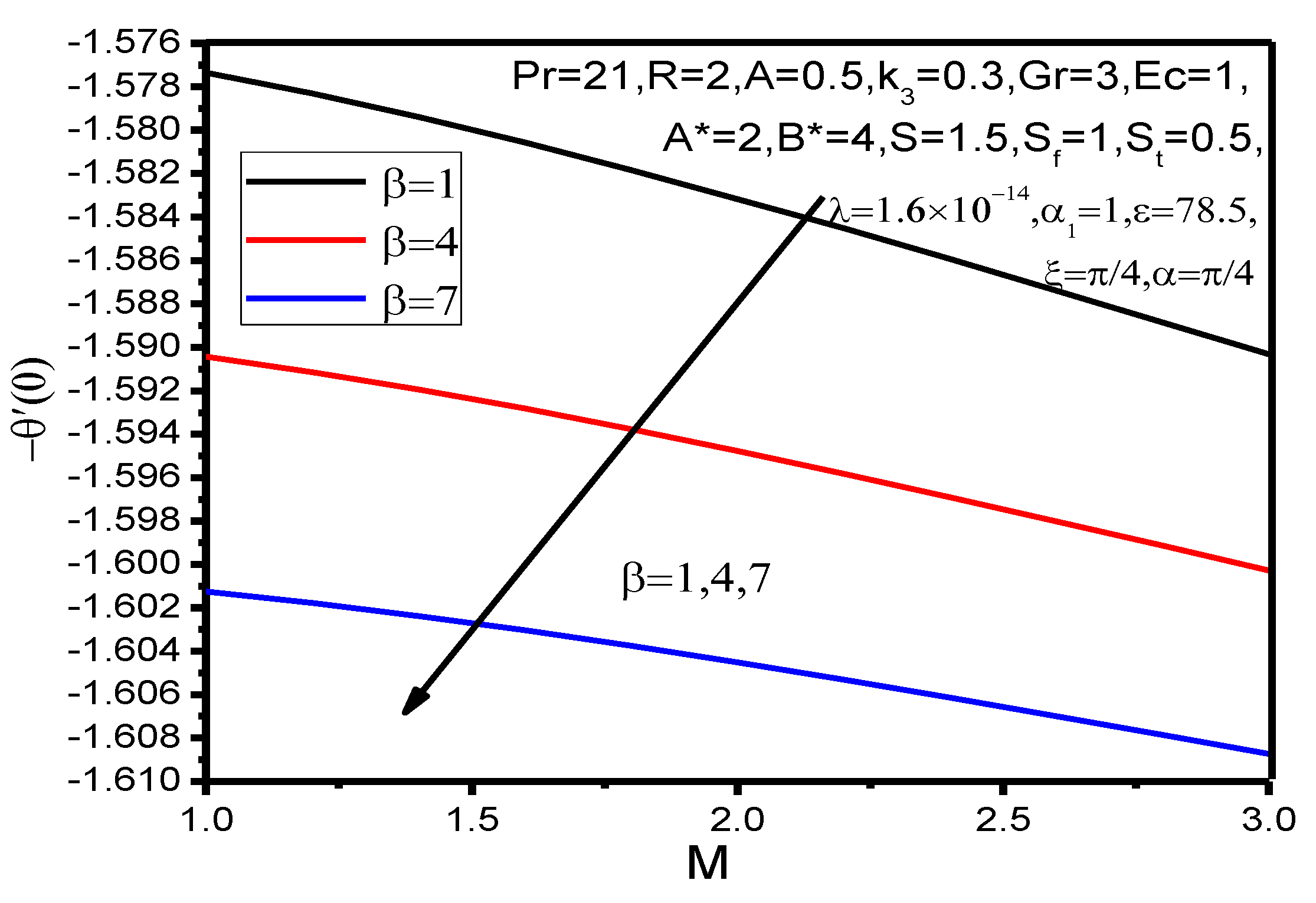
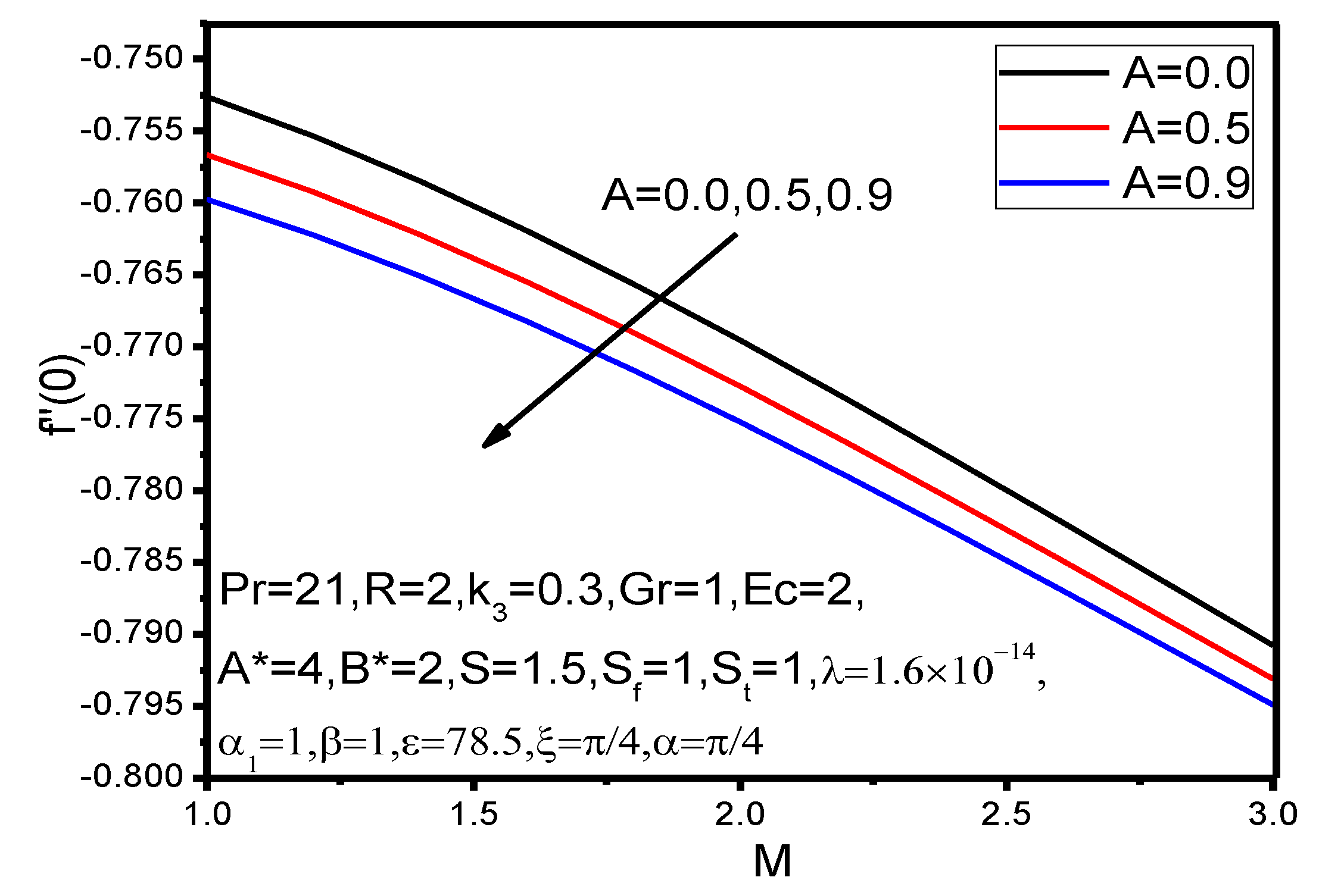
Figure 39 depict the skin friction coefficient and the rate of wall heat transfer with regard to the magnetic parameter for various values of the inclination angle of the sheet, angle of the magnetic field, radiation parameter, ferromagnetic parameter, unsteadiness parameter, and Eckert number. From the figures, it can be observed that skin friction decreases with increasing values of the inclination angle of the sheet and the acute angle of magnetic field, whereas the rate of the wall heat transfer is increased in these cases. Moreover, both skin friction and the rate of wall heat transfer are decreased with increasing values of the radiation parameter, ferromagnetic parameter, and unsteadiness parameter. Moreover, both skin friction and the rate of wall heat transfer are increased with increasing values of the Eckert number.


 and
and 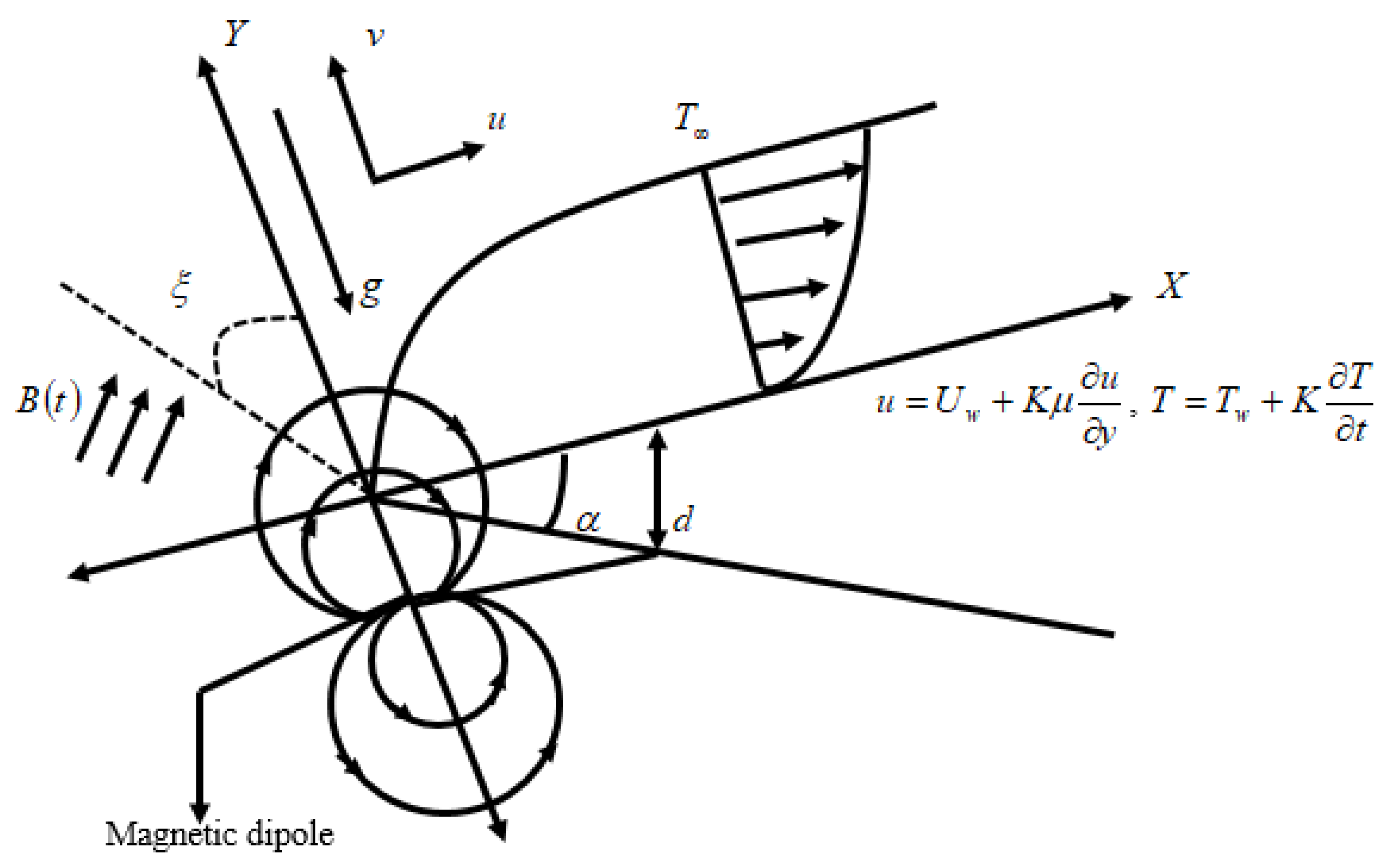


